Estimating Shifts in Phenology and Habitat Use of Cobia in Chesapeake Bay Under Climate Change
 Daniel P. Crear
 Brian E. Watkins
  Marjorie A. M. Friedrichs
- Virginia Institute of Marine Science, William & Mary, Gloucester Point, VA, United States
Cobia (Rachycentron canadum) is a large coastal pelagic fish species that represents an important fishery in many coastal Atlantic states of the U.S. They are heavily fished in Virginia when they migrate into Chesapeake Bay during the summer to spawn and feed. These coastal habitats have been subjected to warming and increased hypoxia which in turn could impact the timing of migration and the habitat suitability of Chesapeake Bay. With conditions expected to worsen, we project current and future habitat suitability of Chesapeake Bay for cobia and predict changes in their arrival and departure times as conditions shift. To do this we developed a depth integrated habitat model from archival tagging and physiology data from cobia that used Chesapeake Bay, and applied the model to contemporary and future temperature and oxygen output from a coupled hydrodynamic-biogeochemical model of Chesapeake Bay. We found that estimated arrival occurs earlier and estimated departure time occurs later when temperatures are warmer and that by mid- and end-of-century cobia may spend on average up to 30 and 65 more days, respectively, in Chesapeake Bay. By mid-century we do not expect habitat suitability to change substantially for cobia, but by end-of-century we project it will significantly decline and shift closer to the mouth of Chesapeake Bay. Our study provides evidence that cobia will have the capacity to withstand near term impacts of climate change, but that their migration phenology varies from year to year with changing temperatures. These findings emphasize the need to incorporate the relationship between fishes and their environment into how fisheries are managed. This information can also help guide managers when deciding the timing and allocation of a fishery.
Introduction
Cobia (Rachycentron canadum) is a large coastal pelagic fish species that uses waters along the mid- and south- Atlantic regions of the U.S. east coast throughout the year. Along the east coast of the U.S., cobia migrate into bays and estuaries, such as Chesapeake Bay, in late spring/early summer to spawn and feed (Joseph et al., 1964; Smith, 1995; Perkinson et al., 2019). They remain in these habitats until late summer/early fall when they migrate primarily offshore to the shelf waters ranging from North Carolina to Florida (Crear et al., 2020b). The exact timing of both inshore and offshore migrations fluctuate each year and are thought to be driven by temperature cues (Smith, 1995; Lefebvre and Denson, 2012). Anecdotal evidence from fishermen suggests that cobia have been entering Chesapeake Bay earlier in recent years, consistent with habitat suitability models suggesting that future climate warming will result in arrival into inshore habitats, like Chesapeake Bay, earlier in the spring (Crear et al., 2020b).
Cobia support a valuable recreational fishery on the U.S. east coast from Florida to Virginia. Estimated cobia landings from the recreational fishery occur primarily in Virginia or North Carolina state waters (SEDAR, 2020). With an average of approximately 225,000 cobia trips occurring annually in Virginia alone, valued between $488–$685 per trip (Scheld et al., 2020), the cobia fishery is extremely important for coastal states like Virginia. In recent years, estimated landings exceeded the Atlantic cobia allowable catch limits, which led the National Marine Fisheries Service (NMFS) to close the fishery in federal waters (NCDENR, 2016; NMFS, 2017). Despite the closure in federal waters, the cobia fishery remained open in state waters (within 3 nautical miles of the coast) because of the importance of the cobia fishery to many coastal states.
Warming within these ecologically and economically important inshore habitats has been occurring and is expected to intensify in the future with climate change (Najjar et al., 2010). As a result of atmospheric warming we expect to see an approximately 2°C increase by mid-century and a 5°C increase by end-of-century in Chesapeake Bay inferred from Saba et al. (2016) and Muhling et al. (2018).
Being adjacent to human populations, coastal habitats like Chesapeake Bay are often impacted by anthropogenic inputs (Brown et al., 2018). Specifically, anthropogenic nutrient inputs combined with warming waters has led to an increase in the extent and severity of hypoxic regions within Chesapeake Bay (Hagy et al., 2004; Rabalais et al., 2009; Najjar et al., 2010). We expect that as climate change continues these impacts will be exacerbated. Irby et al. (2018) project that the largest increase in cumulative hypoxic volume in Chesapeake Bay will occur between oxygen concentrations of 2–5 mg l–1. With an increase in 2 and 5°C and corresponding solubility changes, phytoplankton growth rates, and organic matter remineralization, Chesapeake Bay is expected to see estimated reductions in dissolved oxygen of 0.5 and 1.5 mg l–1 by mid-century and end-of-century, respectively (Irby et al., 2018). These environmental changes may impact the suitability of Chesapeake Bay for cobia and could affect their arrival and departure time, a trend that has been seen in other migratory species (Sims et al., 2004; Jansen and Gislason, 2011).
The relationship between fish physiology and the environment is one way to understand the impacts of climate change on fish. A recent physiology study found that cobia are able to withstand temperatures as warm as 32°C; however, when exercised to exhaustion in these conditions, 30% of individuals suffered mortality (Crear et al., 2020a). Furthermore, this study showed cobia had a very high hypoxia tolerance, where individuals could tolerate oxygen levels as low as 1.7–2.4 mg l–1 at temperatures between 24 and 32°C (Crear et al., 2020a). Based on these results, it appears cobia are more hypoxia tolerant than many active predatory species and therefore might be less impacted by future decreases in dissolved oxygen concentration.
Habitat modeling has been used to assess the impacts of climate change on a number of marine species (Pinsky et al., 2013; Muhling et al., 2016; Kleisner et al., 2017; Morley et al., 2018; McHenry et al., 2019; Crear et al., 2020c). These studies have been used to identify both habitat reductions and range shifts. Although a recent study assessed climate impacts on cobia distribution along the U.S. east coast (Crear et al., 2020b), the spatial resolution of the analysis was too coarse to assess the changes in the habitat quality of Chesapeake Bay.
To predict future changes in phenology and habitat suitability for cobia within the Chesapeake Bay, we developed a habitat model parameterized with our physiology data (Crear et al., 2020a) and archival tagging data. This model was used to project the current arrival and departure times of cobia into Chesapeake Bay and the changes to this phenology in the future under climate change. In addition, our model was used to project changes in habitat suitability in Chesapeake Bay as a function of temperature and oxygen concentration.
Materials and Methods
Tagging
Cobia were caught on rod and reel using typical recreational methods in Chesapeake Bay during the 2017–2018 summer months. Cobia were placed upside down in a V-board, and a hose with water pumping through it was inserted into the mouth. Cobia were measured and tagged by making a 2 cm incision in the abdominal wall, and inserting two tags. The first tag was an acoustic transmitter (V16-4L/4H coded transmitter, 16 mm diameter x 68 mm long, pulse interval 30–120 s, estimated battery life 1,613–3,650 days, 152–158 dB, 24 g in air, Vemco Inc., herein referred to as an “acoustic tag”). The second tag was a data storage tag (G5 data storage tag, 8 mm diameter x 31 mm long, 2.7 g in air, Cefas Technology Limited, herein referred to as a “data logger”), which was programmed to record temperature every 20 min and depth every 1 min for 2 years. A conventional tag was fixed to the data logger and designed to protrude from the incision to alert fishers that caught a tagged fish that a data logger was present inside the fish and that a monetary reward would be given if the tag was returned. The incision was closed with 3 interrupted sutures (PDS II) or 5–8 staples (Conmed Reflex One Skin). An external dart tag was inserted at the base of the dorsal fin. Fish were immediately released following tagging unless the fish appeared lethargic. When this occurred, we held the fish underwater as the boat moved forward slowly to irrigate the gills until the fish was able to swim off on its own. All fish capture, handling, and surgical procedures were approved by the College of William & Mary Institutional Animal Care and Use Committee (protocol no. IACUC-2017-05-26 133-kcweng).
Habitat Model
The habitat model followed similar methods described in Eveson et al. (2015) and Crear et al. (2020b), which uses the ratio between habitat use and habitat availability to determine habitat suitability of the fish species. Habitat use was characterized by the temperatures utilized by tagged cobia (section “Habitat Use Densities” below) and habitat availability was the thermal distribution of the environment, as predicted via biogeochemical modeling (section “Habitat Availability Densities” below). A value greater than 1 indicates suitable conditions (i.e., the conditions the fish occupied occurred in a greater proportion than those conditions in the available habitat data), below 1 indicates unsuitable conditions, and equal to 1 represents no difference than random. In addition to the data from the data loggers, we used the environmental conditions simulated by the three-dimensional (3D) ChesROMS-Estuarine-Carbon-Biogeochemistry (ECB) model. This coupled hydrodynamic-biogeochemical model had a horizontal resolution of approximately 1 km × 1 km and 20 terrain-following vertical levels (i.e., depth levels that follow the contour of the bottom) (Shchepetkin and McWilliams, 2005) that have a higher vertical resolution near the surface and bottom of the water column (Feng et al., 2015; Da et al., 2018; Irby et al., 2018). The results from the ChesROMS-ECB model had three uses: estimates of habitat availability (daily outputs), for predictions of arrival and departure time of cobia to and from Chesapeake Bay over contemporary and future time periods (daily outputs), and for habitat suitability predictions over contemporary and future time periods (across summer averages). Details of the complete habitat model are described below in six steps (Figure 1).
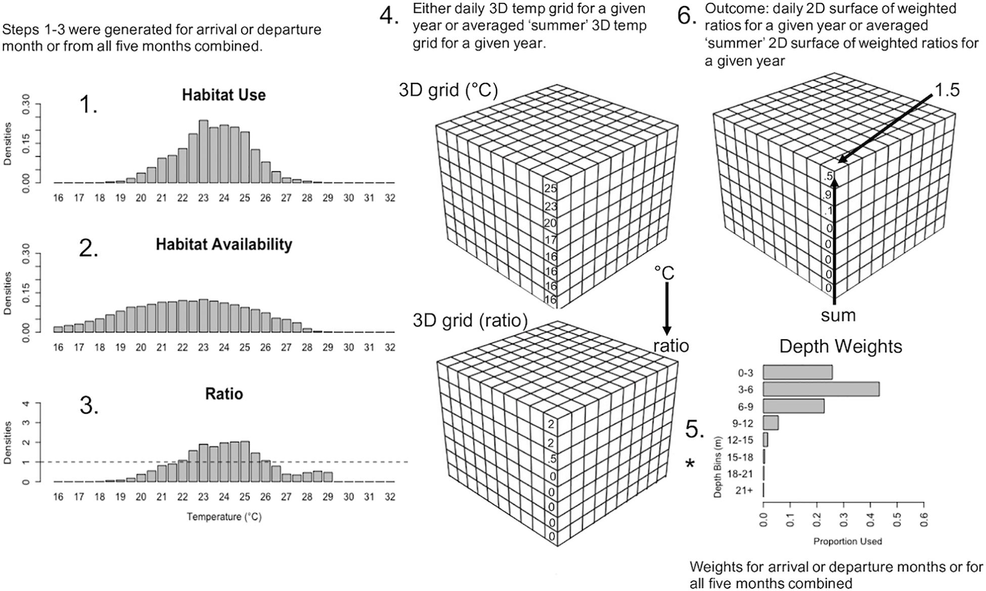
Figure 1. Schematic of the habitat model and how Chesapeake Bay temperature data for specific time periods were run through it. Step 1: Histogram of habitat use densities from data loggers of tagged fish in Chesapeake Bay averaged over a specified time period; 2 arrival months (May, Jun.), 2 departure months (Aug., Sept.), and all 5 summer months combined (May–Sept.). Step 2: Histogram of habitat availability densities generated from daily 3D temperature arrays from Chesapeake Bay (ChesROMS-ECB model), summarized vertically into eight depth bins combined for each of the aforementioned time periods. Step 3: Ratios generated by dividing habitat use densities by habitat availability densities for each time period. Step 4: Either daily 3D arrays (for arrival and departure months) or 3D arrays averaged across two summer periods (May 15–Sept. 30 and Jun. 1–Aug. 31) were extracted from the ChesROMS-ECB model and ratios from Step 3 were assigned to each grid cell at each depth bin based on temperature in that grid cell. Step 5: The vertical habitat distribution of fish in Chesapeake Bay from data loggers was used to generate a depth weighting factor for the above eight depth bins, for each time period. The ratios generated in Step 4 were then multiplied (*) by the appropriate depth weighting factor based on each ratio’s depth in each grid cell for each time period. Step 6: Sum the weighted ratios through the water column to get daily 2D surfaces of weighted ratios for arrival months (May, Jun.) and departure months (Aug., Sept.) for each year and yearly 2D surfaces of weighted ratios for the two summer periods (May 15–Sept. 30 and Jun. 1–Aug. 31).
1. Habitat Use Densities
Habitat use data came from the data loggers and was defined as the temperatures occupied by tagged cobia when the fish were in Chesapeake Bay. Presence inside and outside Chesapeake Bay was determined using the acoustic detections from these fish that were detected on acoustic receiver stations at the mouth of Chesapeake Bay (75.98°W). A fish was deemed inside Chesapeake Bay from when the fish was first detected west of 75.98°W to the last time the fish was detected west of 75.98°W. This method was selected because there was not an acoustic array with a fine enough resolution to determine when the fish was outside Chesapeake Bay. Data within the first 24 h of tagging and during the day of recapture were removed from each fish’s dataset to disregard handling and tagging stress behaviors. Temperature and depth data were summarized by hour for each fish over a specified time range. Densities were extracted from temperature histograms with 0.5°C bins ranging from 1.5 to 33.5°C for each fish. The densities for each temperature were averaged over all fish present in Chesapeake Bay over a specified time range. These histograms and densities were generated for the months cobia arrive to (May and June) and depart from (August and September) Chesapeake Bay, as well as over all 5 months of Chesapeake Bay occupancy (May–September) combined. These densities were considered habitat use for cobia in Chesapeake Bay.
2. Habitat Availability Densities
Habitat availability information for Chesapeake Bay were temperatures and oxygen derived daily from the ChesROMS-ECB model for the time cobia are typically found in ChesapeakeBay (May 15–September 30) over the summers tagged cobia were at-liberty (2017–2019). We did not want to include all of May because the available temperatures would be skewed lower than what is actually available to cobia during the second half of May. Because the vertical levels in the model are not equally spaced, we generated eight depth bins at 3 m intervals (0–3 m, 3–6 m, 6–9 m, 9–12 m, 12–15 m, 15–18 m, 18–21 m, 21+ m). To allow each depth to be treated equally, all temperatures for a given latitude and longitude from levels within a depth bin were averaged over each day. To integrate cobia hypoxia tolerance quantified in Crear et al. (2020a), we removed those portions of the dataset corresponding to physiologically uninhabitable waters. These experiments showed that hypoxia tolerance declines in warmer waters (Crear et al., 2020a). To remove those portions where habitats were physiologically unavailable to cobia, we adjusted cells from depth bins to not available values (NAs) where temperatures were between 24 and 28°C and dissolved oxygen levels were less than or equal to 1.7 mg l–1, where temperatures were greater than 28°C and less than 32°C and dissolved oxygen levels were less than or equal to 2 mg l–1, and where temperatures exceeded 32°C and dissolved oxygen levels were less than 2.4 mg l–1 (Crear et al., 2020a). Because salinity preference is unknown for adult cobia while inhabiting Chesapeake Bay, we generated an area based on where cobia are caught while in Chesapeake Bay. This area extended slightly north of the mouth of the Potomac River (38.10°N) and excluded all areas in Chesapeake Bay tributaries (James, York, Rappahannock, and Potomac Rivers). We also excluded ocean waters, i.e., those east of the Chesapeake Bay mouth at 75.98°W. From here on, this region will be referred to as “Chesapeake Bay.” The accuracy of the ChesROMS-ECB model has not been well-evaluated in shallow depths; therefore, any cells where bottom depths were less than 3 m were not included in these data. All temperatures over all eight depth bins for a specified time period were combined and a histogram and accompanying densities were created from 1.5 to 33.5°C with 0.5°C bins. These densities were generated for the months cobia arrive to (May and June) and depart from (August and September) Chesapeake Bay, as well as over all 5 months (May 15–September) combined. These densities were considered habitat availability for cobia in Chesapeake Bay.
3. Create Ratios
Ratios were calculated for each arrival month (May and June) and departure month (August and September) by dividing the corresponding habitat use densities by the habitat availability densities for those months. Ratios were also calculated from habitat use and habitat availability densities for all 5 months combined. Together this resulted in five sets of ratios (May, June, August, September, and all months combined).
4. Apply Ratios to 3D Habitat
The contemporary and future Chesapeake Bay habitats to predict over were derived from the ChesROMS-ECB model simulation. Daily 3D gridded arrays of temperature and oxygen over a 20-year time period (2000–2019) were considered to represent the contemporary habitat. We generated two future habitat scenarios predicted to occur by mid-century and end-of-century within Chesapeake Bay by adding deltas to the contemporary habitat data. We selected the mid-century deltas to be +2°C and −0.5 mg/l and the end-of-century deltas to be +5°C and −1.5 mg/l (based on Irby et al., 2018). It is important to mention that, similar to Irby et al. (2018), deltas were not selected to reflect any particular Representative Concentration Pathway (RCP) scenario or global climate model (GCM), but to more generally represent what is believed will occur by mid- and end-of-century and thus understand cobia’s sensitivity to these changes. Deltas were applied to all 20 years and evenly over horizontal space and throughout the entire water column since observations suggest that climate change impacts temperatures along the north/south gradient and the temperature of the surface and bottom waters of Chesapeake Bay similarly (Preston, 2004; Irby et al., 2018; Hinson et al., in review). These 3D arrays were then summarized into the eight predefined depth bins and the other adjustments to the arrays described above (section “Habitat Availability Densities”) were also done here. This resulted in daily 3D gridded arrays for three different 20-year timeseries, for contemporary, mid-century, and end-of-century.
To represent arrival (May and June) and departure months (August and September) daily 3D temperature arrays for each year were used. To represent the summer in Chesapeake Bay, the temperature arrays were averaged across days for all 5 months (May 15–September 30) and averaged across days for June 1–August 31 (months when cobia most heavily occupy Chesapeake Bay) for each year. Ratios for the arrival and departure months were then assigned to each grid cell at each depth bin based on the daily temperature in that grid cell and given month for all 20 years. Ratios for the 5 months combined were applied to the two average temperature arrays (5 months combined and June–August combined) based on the temperature in that grid cell at each depth bin for each year.
5. Weight Ratios by Depth
To produce a single ratio value for each latitude and longitude, depth weighting factors were generated for the arrival and departure months and for all 5 months when cobia were present in Chesapeake Bay. The depth weighting factor was calculated by taking the proportion of hourly depth observations from the data loggers at each of the eight depth bins for the arrival and departure months and for all 5 months combined. Based on specified time period and the depth bin the ratio was in, the ratio was multiplied by the appropriate depth weighting factor. For example, if the ratio at a specific latitude and longitude was 2 at the 3–6 m depth bin in June and the depth weighting factor at 3–6 m was 0.5 in June, then the new weighted ratio would be 1.0 at the 3–6 m depth bin in June.
6. Sum Ratios Through Water Column
Once all ratios were weighted, the eight weighted ratios were summed through the water column at each grid cell for each month (May, June, August, and September) and the two arrays of combined months. This resulted in daily 2D surfaces of weighted ratios for May, June, August, September for each year and yearly 2D surfaces of weighted ratios for the May 15–September 30 time period and June 1–August 31 time period. Suitable habitat was considered to be any cell within the Chesapeake Bay habitat where the predicted ratio was greater than 1. Any predicted ratios below 1 were considered unsuitable habitat and any equal to 1 were considered no preference.
Arrival/Departure Analysis
To determine arrival and departure time of cobia in Chesapeake Bay we calculated available suitable habitat in Chesapeake Bay each day from May 1 to June 30 (for arrival) and August 1 to September 30 (for departure) for each year (2000–2019). To do this, the number of grid cells in the Chesapeake Bay area with predicted ratio values greater than 1 were tallied. Arrival day was considered the first date in May or June where greater than 50% of the cells were deemed suitable (>1). Departure day was considered the first date in August or September where less than 50% of the habitat was deemed suitable. We selected a 50% threshold because it estimated dates that fell within one standard deviation of the mean arrival and departure dates for cobia that were acoustically tagged. Specifically, we focused on departures in 2018 and arrivals in 2019 when there were 33 and 32 acoustically tagged cobia that left and entered Chesapeake Bay, respectively. To accommodate expected warming in our future scenarios, we extended Chesapeake Bay cobia habitat projections into April (for arrival) and October (for departure). There were very little or no contemporary habitat use data for cobia in Chesapeake Bay for the months of April and October; therefore ratios and depth weighting factors from May and September were used to predict over mid-century and end-of-century habitat in April and October, respectively.
To assess if arrival or departure day significantly changed over the current 20 year period (2000–2019) or over temperature we ran two linear models. The response variables were estimated yearly arrival day relative to May 1st and estimated yearly departure day relative to September 1st, for the arrival and departure model, respectively. The fixed effects for the arrival model were overall mean May water temperature in Chesapeake Bay each year and year, while the fixed effects for the departure model were overall mean September water temperature in Chesapeake Bay each year and year. Linear mixed effects models were run to determine if arrival and departure dates differed over the contemporary, mid-century, and end-of-century time periods using the nlme package (Pinheiro et al., 2013). For these models, the response variables were again estimated arrival day and estimated departure day for each year, for the arrival and departure model, respectively. The fixed effect was time period, while the random effect was year (2000–2019) in these models. Tukey’s post-hoc tests were run to determine differences among the time periods. All statistics were evaluated at a significance level of α = 0.05.
Habitat Suitability
The yearly 2D predicted ratio surfaces generated from the two summer periods (May 15–September 30; June 1–August 31) for each of the three time periods (contemporary, mid-century, and end-of-century) were used to calculate habitat suitability values for Chesapeake Bay. The predicted ratio values greater than 1 were summed over Chesapeake Bay for each year of each time period for each summer period to get yearly total habitat suitability index values. A linear mixed effects model was used to determine whether total habitat suitability index changed through each long term time period (contemporary, mid-century, and end-of-century) for the two summer periods (May 15–September 30; June 1–August 31). An interaction was used between these two fixed effects, long term time period and the two summer time periods, while the response variable was total habitat suitability index each year. Year was a random effect in this model. All R code for modeling and statistical analyses can be found in the Supplementary Material.
Results
Data Retrieval
We received eight data loggers from fishermen. These eight fish ranged from 78.7 to 139.7 cm total length (mean ± SD: 106.0 ± 18 cm) (Table 1). Days-at-liberty within Chesapeake Bay ranged from 26 to 151 days (92 ± 46) days, yielding a total of 736 days of data.
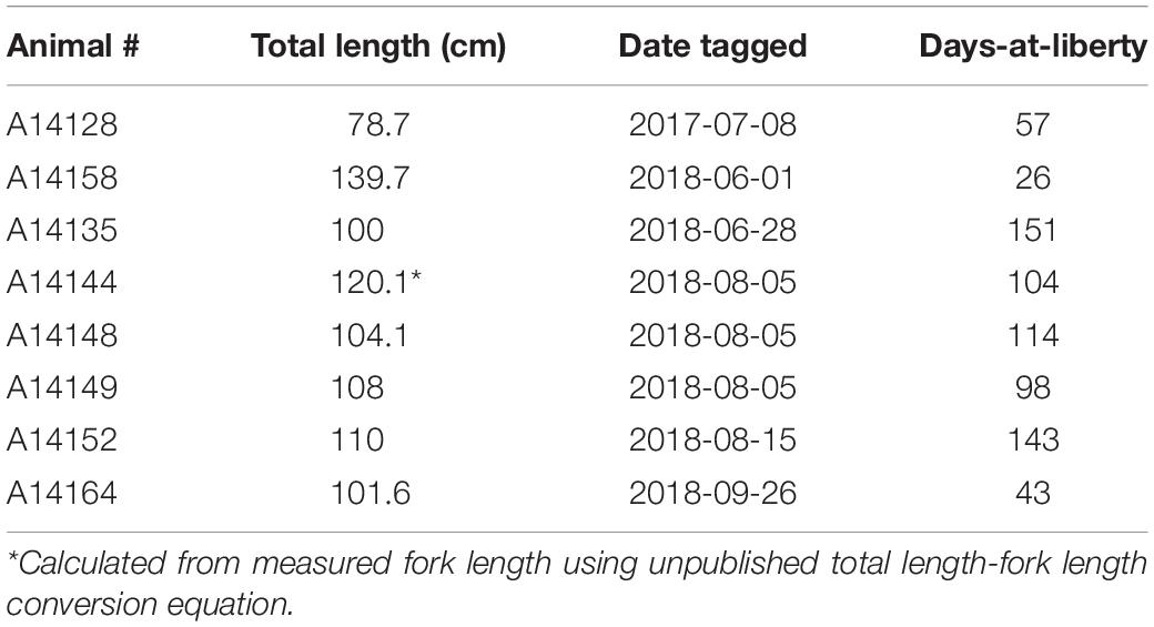
Table 1. Tag information for cobia tagged with a G5 data storage tag (Cefas), including total length when tagged, tagging date, and days-at-liberty in Chesapeake Bay.
Habitat Model
Habitat suitability ratios were generated for each arrival month (May and June), for each departure month (August and September), and for all summer months combined. During arrival and departure months, cobia preferred temperatures from 21.5 to 27°C and 24.5 to 31°C, respectively. Over the entirety of the summer cobia preferred 22.5–28°C (Figure 2). Depth weighting factors were generated for each arrival and departure month and for all summer months combined. During early arrival (May) cobia preferred 0–6 m, but later into June cobia selected 0–9 m. During early departures (August) cobia were observed between 0 and 9 m, but during September cobia were most common at slightly deeper depths (0–12 m). When all summer months were combined, cobia were observed most frequently at depths between 0 and 9 m (Figure 3).
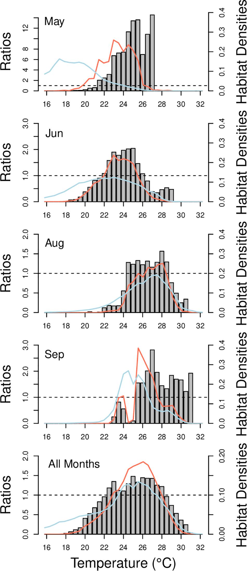
Figure 2. Habitat suitability ratios from 16 to 32°C for each arrival month (May and June), departure month (August–September), and all summer months combined for when cobia were inside Chesapeake Bay (May–September). The ratios were developed from dividing the habitat use densities (red lines) by the habitat availability densities (blue lines) at each temperature during times when cobia were inside Chesapeake Bay. Dashed lines is at a ratio of 1.0.
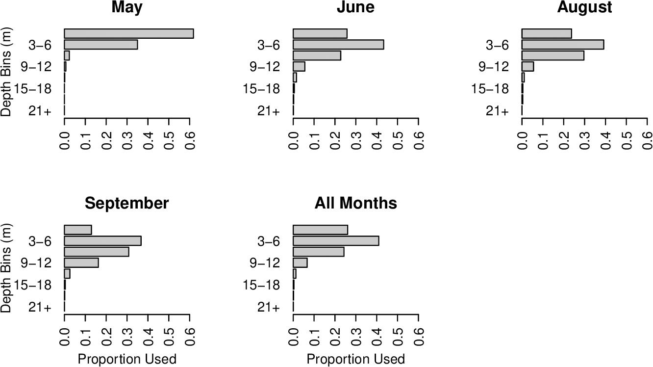
Figure 3. Depth weighting factors for each 3 m depth bin for each arrival month (May and June), departure month (August and September), and all summer months combined (May–September).
Arrival/Departure
Estimated cobia arrival time fluctuated over the last 20 years. Although there was no significant trend (t = −0.52, p > 0.05), in more recent years it appears that cobia have been arriving earlier in the year. For example, the mean estimated arrival time between earlier years (2000–2004) was 29.2 days since May 1st (all arrival values from here on are relative to May 1st), but 23.0 days for later years (2015–2019) (Figure 4A). Estimated arrival time significantly decreased (t = −5.4, p < 0.001) as average May temperature increased. Specifically, for every °C increase, arrival time occurred 8.6 days earlier in the Spring (Figure 4B). Arrival time significantly differed [F(2, 38) = 106.6, p < 0.001] among time periods (contemporary, mid-century, end-of-century; Figure 4C), where contemporary mean arrival time (mean ± SD; 27.8 ± 9.0 days) significantly differed from mid-century arrival time (16.0 ± 7.9 days; p < 0.05) and end-of-century arrival time (−1.5 ± 7.0 days; p < 0.05). Arrival times for mid-century and end-of-century also significantly differed (p < 0.05).
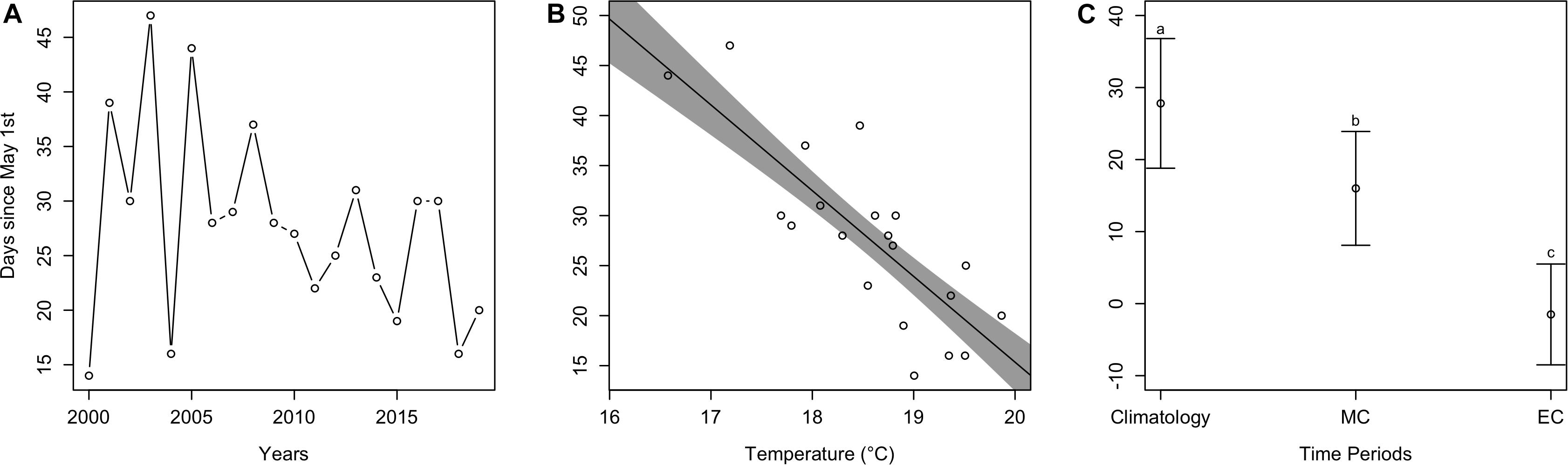
Figure 4. Estimated arrival plots. (A) Estimated arrival time of cobia each year from 2000 to 2019. (B) The dots represent estimated cobia arrival times over mean May temperatures in Chesapeake Bay, while the line and shaded region represent model output and uncertainty. (C) Mean estimated cobia arrival time among climatology (i.e., contemporary), mid-century (MC), and end-of-century (EC) time periods. Different lower case letters indicate a statistical difference between time periods.
Similar to arrival time, estimated departure time relative to September 1st (all departure values from here on are relative to September 1st) also varied over the last 20 years, and there was no significant trend (t = 0.23, p > 0.05). Despite this, the mean estimated departure time between earlier years was 3.0 days since September 1st, but 15.4 days for later years (Figure 5A). As average September temperature increased, estimated departure time significantly increased (t = 6.0, p < 0.001), where for every °C increase, departure time occurred 9.4 days later in the Fall (Figure 5B). Estimated departure time also significantly differed among time periods [F(2, 38) = 154.6, p < 0.001; Figure 5C]. Specifically, contemporary mean departure time (10.1 ± 8.3 days) significantly differed from mid-century (27.7 ± 10.6 days; p < 0.05) and end-of-century (45.2 ± 6.7 days; p < 0.05). Departure times for mid-century and end-of-century significantly differed as well (p < 0.05).
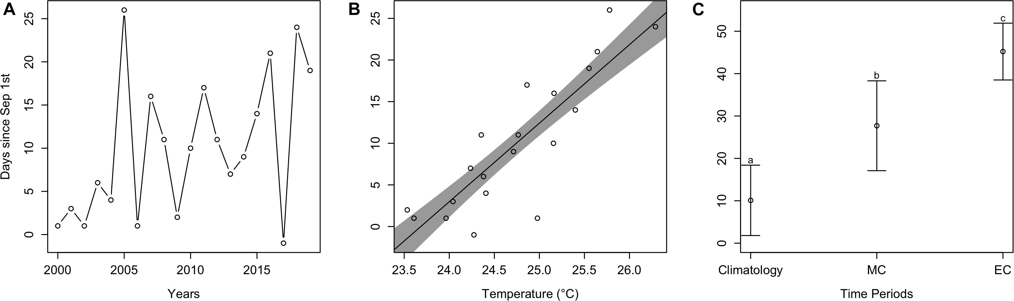
Figure 5. Estimated departure plots. (A) Estimated departure time of cobia each year from 2000 to 2019. (B) The dots represent estimated cobia departure times over mean September temperatures in Chesapeake Bay, while the line and shaded region represent model output and uncertainty. (C) Mean estimated cobia departure time among climatology (i.e., contemporary), mid-century (MC), and end-of-century (EC) time periods. Different lower case letters indicate a statistical difference between time periods.
Habitat Suitability
An interaction between long term time period (contemporary, mid-century, end-of-century) and the two summer time periods (May 15–September 30; June 1–August 31) significantly affected total habitat suitability index [F(2, 95) = 25.1, p < 0.001]. The most suitable habitat during June-August for cobia in Chesapeake Bay spans from north of the James River all the way to the northern extent of the study region (north of the Potomac River) for the contemporary time period (Figure 6A). Despite the lack of a significant difference between the total habitat suitability index for the two summer time periods (p > 0.05; Figure 7), mean habitat suitability does appear to decline slightly throughout most of the Chesapeake Bay cobia region when we incorporated days in May and all of September (Figure 6D). Mean habitat suitability from June-August, during mid-century shifted further south, closer to the mouth compared to the contemporary period (Figure 6B). In addition, the total habitat suitability index significantly decreased between the contemporary and mid-century periods for June-August (p < 0.05; Figure 7). However, when assessing May 15–September 30 during mid-century, total habitat suitability index did not decline relative to the contemporary period. Although there is no significant difference, it does appear that total habitat suitability index increased slightly by mid-century (p > 0.05; Figure 7). This is also reflected in habitat improvements over much of Chesapeake Bay (Figure 6E). Total habitat suitability index also significantly differed between the two summer periods during mid-century (p < 0.05; Figure 7). For end-of-century, we project a significant decrease in suitable cobia relative to mid-century for June-August (p > 0.05) and May 15–September 30 (p > 0.05; Figure 7). This is reflected in habitat loss throughout most of Chesapeake Bay and a shift toward the bay’s mouth (Figures 6C,F). Total habitat suitability index was also significantly lower for June-August compared to May 15–September 30 (p < 0.05; Figure 7).
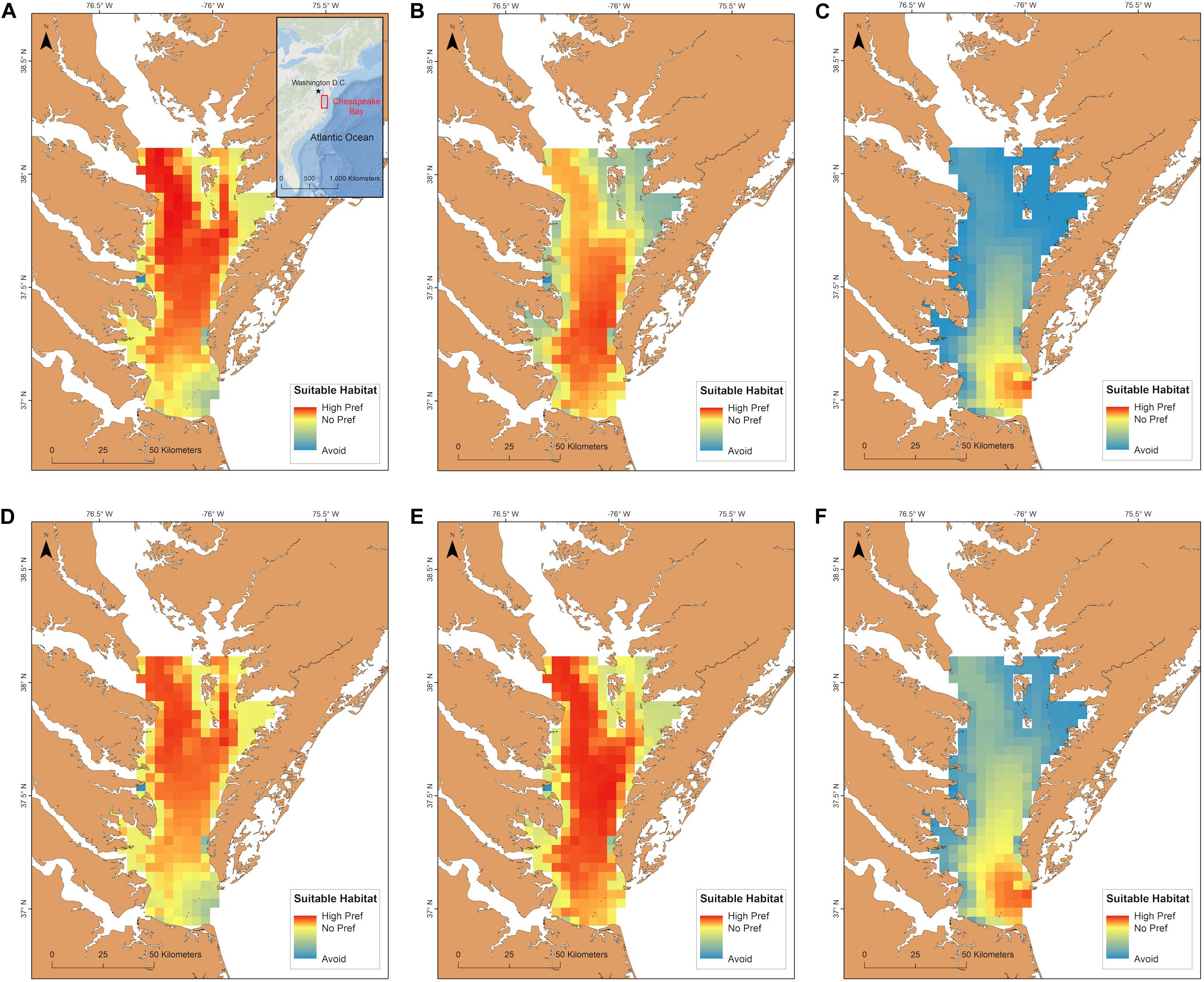
Figure 6. Cobia habitat suitability within Chesapeake Bay averaged over years for the contemporary (A,D), mid-century (B,E), and end-of-century (C,F) time periods. The first row is mean habitat suitability for June-August (a-c) and the second row is mean habitat suitability for May 15–September 30 (D–F).
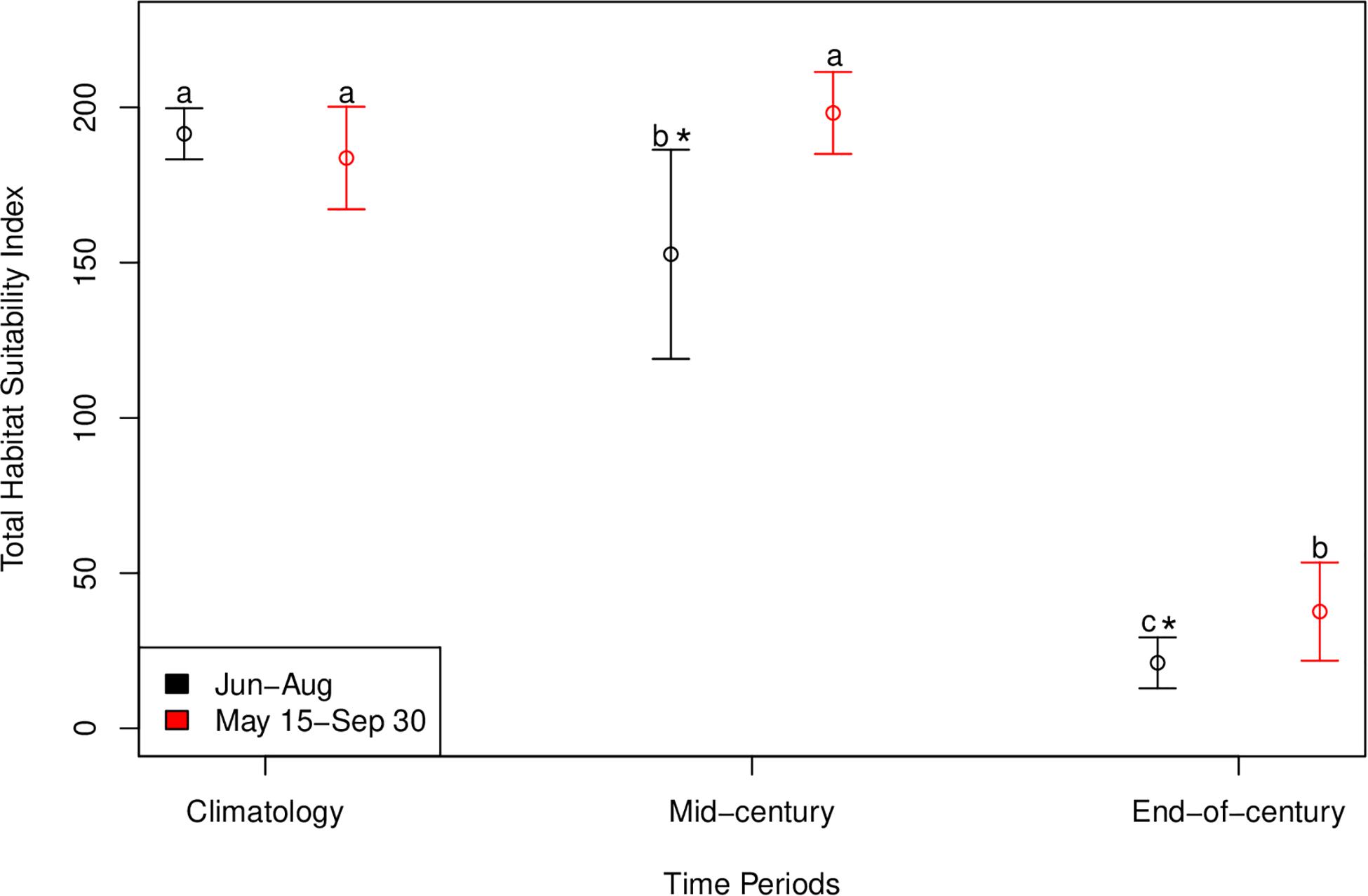
Figure 7. Total habitat suitability index for cobia in Chesapeake Bay during contemporary, mid-century, and end-of-century time periods for each summer period (Jun–Aug and May 15–Sep 30). Error bars represent standard deviation. Black symbols represent the mean total habitat suitability index values for June–August and red symbols represent the mean total habitat suitability index values for May 15–September 30. Different lower case letters indicate a statistical difference among time periods within a summer period. For example, in the Jun-Aug summer period all three times periods are different from one another. An * indicates a statistical difference between summer periods within a time period.
Discussion
This study presents the first attempt at describing the distribution of cobia within Chesapeake Bay. We generated a depth integrated habitat model to predict contemporary and future distributions of cobia within Chesapeake Bay using temperature, dissolved oxygen, and depth. By developing a novel model incorporating 3D habitat and physiology, we limit our model variables to those that are available in 3D, but we felt it was more important to incorporate depth than include other variables (many of which are not available at a fine enough resolution) because cobia use the entire water column. Although weighting and summarizing by depth has its benefits (e.g., two-dimensional output; patterns more easily discernable), the approach does have some limitations. For example, there may be small pockets of more suitable habitat at various depths (sub-gridscale) that are not expressed in our results and thus could potentially lead to an underestimation in some suitable habitat predictions. While inhabiting Chesapeake Bay, cobia are highly driven by biotic factors, like spawning and feeding, which were not included in our model; however, we believe environmental variables constrain cobia to certain areas in Chesapeake Bay, which are expressed in our model output. Because of this, we only assessed habitat suitability for the entire summer as a whole. The phenology of cobia arrival and departure to Chesapeake Bay appears to be cued by temperature, which then leads to inshore spawning and foraging. Therefore, we believe our temperature driven habitat model is justified in describing cobia phenology. It is important to note that another limitation of this study is the low sample size of cobia used in the model and that individuals used in our model may not be a full representation of cobia that summer Chesapeake Bay. An increase in sample size may lead to shifts in estimated phenology and habitat suitability. Despite this, our phenology estimates fell within one standard deviation of actual departure and arrival days based on over 30 acoustic tagged cobia. Lastly, we also would like to reiterate that the trends estimated from climate change projections are not intended to represent shifts under any RCP scenario or GCM, but more generally demonstrate cobia’s sensitivity to future oxygen and temperature conditions likely to occur around mid- and end-of-century.
Contemporary Trends
It is clear temperature is a major driver of cobia arrival to and departure from Chesapeake Bay. Over the last 20 years, when temperatures were warmer in May, cobia arrived earlier. Tag pop off locations and modeling suggest that cobia overwinter offshore along the U.S. shelf from North Carolina to Florida (Crear et al., 2020b; Jensen and Graves, 2020). Although cobia are unaware of the temperature in Chesapeake Bay when they are in their overwintering offshore waters, warm temperature cues on the shelf are most likely reflected in Chesapeake Bay as well. This has been observed in mackerel, which arrived to their spawning grounds earlier when sea surface temperature was warmer at a rate of −15 ± 12.1 days/°C (Jansen and Gislason, 2011). Although the trend was not significant, it does appear that when comparing estimated arrival time approximately 20 years ago to today, cobia may be migrating into Chesapeake Bay earlier in recent years. Earlier migrations have been recorded in various tuna species as well, which have migrated to feeding grounds up to 14 days earlier over a 25 year period (Dufour et al., 2010).
Once cobia enter Chesapeake Bay in May, the occurrence of high ratio values generated from the habitat use and habitat availability densities and the use of shallower habitats suggest that cobia are likely seeking out the warm shallow habitats until some of the deeper areas (>6 m) warm up. During the main summer months in Chesapeake Bay (June–August), most of the areas in southern Chesapeake Bay appear to be suitable for cobia. The suitability of most of these areas allow cobia to spawn and feed freely without being restricted by less optimal conditions, except for areas that are excluded as a result of low oxygen. However, because cobia have a high hypoxia tolerance the negative impacts of low oxygen is likely minimal. These favorable conditions are ideal for cobia, which are indeterminate batch spawners and are capable of spawning multiple times over the spawning season (Brown-Peterson et al., 2001; Lefebvre and Denson, 2012). To further define cobia habitat use in estuaries, it would be useful for future studies to examine the relationships between cobia and the location of bathymetric features, manmade structure (e.g., buoys and pilings), salinity, tidal currents, and bait schools (e.g., menhaden) all of which are thought (based on anecdotal evidence) to influence cobia movements while inshore.
Typically, once spawning is complete, individuals have foraged, and temperatures cool in Chesapeake Bay, cobia begin their migration out onto the shelf. However, when temperatures in September are warmer than usual, cobia remain in Chesapeake Bay longer. Similar to arrivals, despite no significant trend over time, it appears that in recent years cobia are leaving Chesapeake Bay later compared to 20 years ago. Although we did not directly look at changes in dissolved oxygen levels on cobia phenology, it is likely not a major driver because of cobia’s hypoxia tolerance and the lack of large hypoxic zones during the months they arrive and depart to and from Chesapeake Bay. Overall, these results suggest that cobia phenology has already been impacted by climate change over the last 20 years.
Future Trends
Phenology trends observed over the last 20 years are projected to extend more rapidly in the future as climate change contributes to even warmer conditions. By mid-century and end-of-century, conditions in Chesapeake Bay may allow cobia to arrive by mid-May and late April/early May on average, respectively. Furthermore, departure time is predicted to extend to the end of September and mid-October by mid-century and end-of-century, respectively. When combining the estimated earlier arrival and later departure, our results indicate that cobia may increase their residence time in Chesapeake Bay by an extra 30 days by mid-century and 65 days by end-of-century. Despite this large increase in the number of days, cobia may be faced with more unsuitable habitat during the months when temperatures are the warmest. When combining more favorable conditions during the last 2 weeks of May and all of September, suitable habitat does not change much by mid-century. If climate change continues at its current rate, suitable habitat is expected to decrease significantly and shift closer to the Chesapeake Bay mouth by the end-of-century, even when incorporating the second half of May and all of September. Further, these trends should be interpreted as the average summer cobia distribution, which in turn, could potentially hide periodic marine heatwave events that could result in displacement and further habitat reduction. Future decline in suitable habitat has similarly been projected for many other coastal species (Albouy et al., 2013; Brown et al., 2016). For example, an increase in sublethal temperatures in the San Francisco Estuary as a result of climate change will likely cause behavioral avoidance of these temperatures and considerable habitat reduction for the Delta smelt (Hypomesus transpacificus) (Brown et al., 2016).
Although habitat shifts and community composition has favored warm-adapted species (Howell and Auster, 2012), the predicted occurrence of more extreme temperatures has the capability to negatively impact warm-adapted species like cobia. For example, if cobia migrate into Chesapeake Bay earlier, spawning may occur earlier. This could impact the survival of eggs and larvae, which depend on the timing of specific temperatures and favorable primary production conditions (Durant et al., 2007). On the other hand, if spawning duration is extended and phytoplankton blooms align, larval survival may improve (Kristiansen et al., 2011). If substantial spawning habitat is lost for estuarine species like cobia, we may see populations decline. We may also see species shift their spawning habitat to more poleward estuaries or offshore habitat where conditions are more favorable for spawning adults and larvae. Recent genetic studies suggest that cobia already have a separate offshore spawning group (Darden et al., 2014; Perkinson et al., 2019), meaning cobia have the ability to spawn in offshore waters. Furthermore, Crear et al. (2020b) found that over the next 60–80 years, there will continue to be an increase in the proportion of suitable cobia habitat in state waters (within 3 nautical miles of shore) from Maryland to Massachusetts during the summer spawning months. Likewise, non-warm-adapted species like, Northeast Artic cod (Gadus morhua) have already shifted their spawning habitat further north over the last half a century, a behavior likely linked to climate change (Sandø et al., 2020). If cobia shift their spawning habitat further north or extend their time inshore, they may subsequently shift their overwintering grounds to be closer to their spawning habitat. Because cobia offshore migrations are driven by temperature, we hypothesize that their overwintering grounds are likely plastic. Therefore, although suitable habitat may still be available further south in the winter (Crear et al., 2020b), it may be less energetically costly to migrate off the shelf toward the Gulf Stream instead of migrating to shelf waters between North Carolina and Florida. If further migrations are made, females may be required to divert energy away from egg production to compensate. Although we talk about these impacts being decades away, some of these hypotheses can be tested today as marine heatwaves become more prevalent along the Northeast Shelf.
Cobia may have the ability to behaviorally adapt to climate change within Chesapeake Bay. The fact that cobia could withstand water temperatures as warm as 32°C (Crear et al., 2020a), suggests that if waters warmed throughout Chesapeake Bay, areas with water temperatures up to 32°C could still be habitable or maybe even suitable. Meaning, temperatures between 22.5 and 28°C may be preferred, but if unavailable, cobia could still inhabit warmer temperatures. If this is the case, our projected future habitat suitability maps may underestimate the amount of suitable habitat in Chesapeake Bay. If this is possible, it is still unknown whether other essential functions like growth or reproduction could be compromised.
Management Implications
Hundreds of thousands of recreational fishermen enjoy fishing for cobia each year in Virginia alone and it appears this number has increased in recent years (B. Watkins pers. comm.). As the amount of time cobia spend in Chesapeake Bay increases with climate change, management will need to be prepared for catch increases. In recent years, the fishery in Virginia has been open from June 1 to various dates in September. If the fishing season dates remain the same, we may expect to see an increase in the catch and release of more cobia in May and more cobia retained later in the season. Our study and a previous study (Crear et al., 2020a) suggest cobia have the capacity to withstand near term (+30 years) impacts of climate change, which is a good sign for a fishery that has grown over the last decade.
A dynamic approach to management may prepare managers for the early migrations to or late departures from Chesapeake Bay. Dynamic management provides managers with the opportunity to adjust managed areas temporally and spatially in time when our coastal waters are changing faster than we are accustomed to (Maxwell et al., 2015; Dunn et al., 2016; Welch et al., 2019). Specifically, as the predictability of coastal ocean models improve, we will have the capacity to couple them with our cobia habitat model to project the timing of cobia migrations months to seasons in advance. This information could be used to guide the timing of the fishing season in Virginia and also influence allocation of cobia among states on a broader scale. As fish behaviorally adapt to changing water conditions, it is critical that management be prepared to adapt as well.
Data Availability Statement
The raw data supporting the conclusions of this article will be made available by the authors, without undue reservation, to any qualified researcher.
Ethics Statement
The animal study was reviewed and approved by the College of William & Mary Institutional Animal Care and Use Committee (protocol no. IACUC-2017-05-26 133-kcweng).
Author Contributions
DC substantially contributed to project conception and design, animal tagging, analysis and interpretation of data, and drafting the manuscript. BW contributed to animal tagging and assisted in manuscript revision. MF and PS provided funding support, generated environmental data, and provided manuscript revisions. KW contributed funds to the project, participated in project conception and design, animal tagging, and assisted in manuscript revision. All authors contributed to the article and approved the submitted version.
Funding
Financial support was provided by the VIMS startup funds, Virginia Sea Grant (award # V721500), the National Oceanic and Atmospheric Administration (NOAA) Saltonstall Kennedy Program (award # NA18NMF4270199), the NOAA’s National Centers for Coastal Ocean Science (award # NA16NOS4780207), and the National Science Foundation (award # ACI-1548562).
Conflict of Interest
The authors declare that the research was conducted in the absence of any commercial or financial relationships that could be construed as a potential conflict of interest.
Acknowledgments
We thank many VIMS undergraduates and VIMS graduate students and staff for their help in tagging cobia, including S. Kilmer, B. Gallagher, M. Oliver, J. Martinez, E. Biesack, and B. Hamilton. We especially thank all of the cobia fishermen that helped us catch and tag cobia and for those that returned tags to us. We want to thank R. Gallagher at NCSU for providing some acoustic tagging data for fish that shared our archival tag and their acoustic transmitter. We also thank J. Hartog and T. Patterson for their advice in model design. This work used the Extreme Science and Engineering Discovery Environment (XSEDE) supercomputer Comet at SDSC through allocation OCE-160013. We also acknowledge William & Mary Research Computing (https://www.wm.edu/it/rc) for providing computational resources and/or technical support that have contributed to the results reported within this manuscript. Lastly, we appreciate the input and advice on research contributing to this work from Alistair Hobday and Rich Brill, and comments on the manuscript from the two reviewers. This is Virginia Institute of Marine Science contribution # 3959.
Supplementary Material
The Supplementary Material for this article can be found online at: https://www.frontiersin.org/articles/10.3389/fmars.2020.579135/full#supplementary-material
References
Albouy, C., Guilhaumon, F., Leprieur, F., Lasram, F. B. R., Somot, S., Aznar, R., et al. (2013). Projected climate change and the changing biogeography of coastal Mediterranean fishes. J. Biogeogr. 40, 534–547. doi: 10.1111/jbi.12013
Brown, E. J., Vasconcelos, R. P., Wennhage, H., Bergström, U., Støttrup, J. G., van de Wolfshaar, K., et al. (2018). Conflicts in the coastal zone: human impacts on commercially important fish species utilizing coastal habitat. ICES J. Mar. Sci. 75, 1203–1213. doi: 10.1093/icesjms/fsx237
Brown, L. R., Komoroske, L. M., Wagner, R. W., Morgan-King, T., May, J. T., Connon, R. E., et al. (2016). Coupled downscaled climate models and ecophysiological metrics forecast habitat compression for an endangered estuarine fish. PLoS One 11:e0146724. doi: 10.1371/journal.pone.0146724
Brown-Peterson, N. J., Overstreet, R. M., Lotz, J. M., Franks, J. S., and Burns, K. M. (2001). Reproductive biology of cobia. Rachycentron canadum, from coastal waters of the southern United States. Fish. Bull. 99, 15–28.
Crear, D. P., Brill, R. W., Averilla, L. M., Meakem, S. C., and Weng, K. C. (2020a). In the face of climate change and exhaustive exercise: the physiological response of an important recreational fish species. R. Soc. Open Sci. 7, 1–13. doi: 10.1098/rsos.200049
Crear, D. P., Watkins, B. E., Saba, V. S., Graves, J. E., Jensen, D. R., Hobday, A. J., et al. (2020b). Contemporary and future distributions of cobia. Rachycentron canadum. Div. Distrib. 26, 1002–1015. doi: 10.1111/ddi.13079
Crear, D. P., Latour, R. J., Friedrichs, M. A. M., St-Laurent, P., and Weng, K. C. (2020c). Sensitivity of a shark nursery habitat to a changing climate. Mar. Ecol. Prog. Ser. 652, 123–136. doi: 10.3354/meps13483
Da, F., Friedrichs, M. A. M., and St-Laurent, P. (2018). Impacts of atmospheric nitrogen deposition and coastal nitrogen fluxes on oxygen concentrations in Chesapeake Bay. J. Geophys. Res. Oceans 123, 5004–5025. doi: 10.1029/2018jc014009
Darden, T. L., Walker, M. J., Brenkert, K., Yost, J. R., and Denson, M. R. (2014). Population genetics of Cobia (Rachycentron canadum): implications for fishery management along the coast of the southeastern United States. Fish. Bull. 112, 24–35. doi: 10.7755/FB.112.1.2
Dufour, F., Arrizabalaga, H., Irigoien, X., and Santiago, J. (2010). Climate impacts on albacore and bluefin tunas migrations phenology and spatial distribution. Prog. Oceanogr. 86, 283–290. doi: 10.1016/j.pocean.2010.04.007
Dunn, D. C., Maxwell, S. M., Boustany, A. M., and Halpin, P. N. (2016). Dynamic ocean management increases the efficiency and efficacy of fisheries management. Proc. Natl. Acad. Sci. U S A. 113, 668–673. doi: 10.1073/pnas.1513626113
Durant, J. M., Hjermann, D. Ø, Ottersen, G., and Stenseth, N. C. (2007). Climate and the match or mismatch between predator requirements and resource availability. Clim. Res. 33, 271–283. doi: 10.3354/cr033271
Eveson, J. P., Hobday, A. J., Hartog, J. R., Spillman, C. M., and Rough, K. M. (2015). Seasonal forecasting of tuna habitat in the Great Australian Bight. Fish. Res. 170, 39–49. doi: 10.1016/j.fishres.2015.05.008
Feng, Y., Friedrichs, M. A. M., Wilkin, J., Tian, H., Yang, Q., Hofmann, E. E., et al. (2015). Chesapeake Bay nitrogen fluxes derived from a land-estuarine ocean biogeochemical modeling system: Model description, evaluation, and nitrogen budgets. J. Geophys. Res. 120, 1666–1695. doi: 10.1002/2015jg002931
Hagy, J. D., Boynton, W. R., Keefe, C. W., and Wood, K. V. (2004). Hypoxia in Chesapeake Bay, 1950–2001: long-term change in relation to nutrient loading and river flow. Estuaries 27, 634–658. doi: 10.1007/bf02907650
Howell, P., and Auster, P. J. (2012). Phase shift in an estuarine finfish community associated with warming temperatures. Mar. Coastal Fisher. 4, 481–495. doi: 10.1080/19425120.2012.685144
Irby, I. D., Friedrichs, M. A. M., Da, F., and Hinson, K. E. (2018). The competing impacts of climate change and nutrient reductions on dissolved oxygen in Chesapeake Bay. Biogeosciences 15, 2649–2668. doi: 10.5194/bg-15-2649-2018
Jansen, T., and Gislason, H. (2011). Temperature affects the timing of spawning and migration of North Sea mackerel. Continental Shelf Res. 31, 64–72. doi: 10.1016/j.csr.2010.11.003
Jensen, D. R., and Graves, J. E. (2020). Movements, habitat utilization, and post-release survival of cobia (Rachycentron canadum) that summer in Virginia waters assessed using pop-up satellite archival tags. Anim. Biotele. 8, 1–13.
Joseph, E. B., Norcross, J. J., and Massmann, W. H. (1964). Spawning of the cobia, Rachycentron canadum, in the Chesapeake Bay area, with observations of juvenile specimens. Chesapeake Sci. 5, 67–71. doi: 10.2307/1350791
Kleisner, K. M., Fogarty, M. J., McGee, S., Hare, J. A., Moret, S., Perretti, C. T., et al. (2017). Marine species distribution shifts on the US Northeast Continental Shelf under continued ocean warming. Prog. Oceanogr. 153, 24–36. doi: 10.1016/j.pocean.2017.04.001
Kristiansen, T., Drinkwater, K. F., Lough, R. G., and Sundby, S. (2011). Recruitment variability in North Atlantic cod and match-mismatch dynamics. PLoS One 6:e17456. doi: 10.1371/journal.pone.0017456
Lefebvre, L. S., and Denson, M. R. (2012). Inshore spawning of cobia (Rachycentron canadum) in South Carolina. Fish. Bull. 110, 397–412.
Maxwell, S. M., Hazen, E. L., Lewison, R. L., Dunn, D. C., Bailey, H., Bograd, S. J., et al. (2015). Dynamic ocean management: Defining and conceptualizing real-time management of the ocean. Mar. Policy 58, 42–50. doi: 10.1016/j.marpol.2015.03.014
McHenry, J., Welch, H., Lester, S. E., and Saba, V. (2019). Projecting marine species range shifts from only temperature can mask climate vulnerability. Glob. Change Biol. 25, 4208-4221.
Morley, J. W., Selden, R. L., Latour, R. J., Frölicher, T. L., Seagraves, R. J., and Pinsky, M. L. (2018). Projecting shifts in thermal habitat for 686 species on the North American continental shelf. PLoS One 13, 1–28. doi: 10.1371/journal.pone.0196127
Muhling, B. A., Brill, R., Lamkin, J. T., Roffer, M. A., Lee, S.-K., Liu, Y., et al. (2016). Projections of future habitat use by Atlantic bluefin tuna: mechanistic vs. correlative distribution models. ICES J. Mar. Sci. 74, 698–716. doi: 10.1093/icesjms/fsw215
Muhling, B. A., Gaitán, C. F., Stock, C. A., Saba, V. S., Tommasi, D., and Dixon, K. W. (2018). Potential salinity and temperature futures for the Chesapeake Bay using a statistical downscaling spatial disaggregation framework. Estuaries Coasts 41, 349–372. doi: 10.1007/s12237-017-0280-288
Najjar, R. G., Pyke, C. R., Adams, M. B., Breitburg, D., Hershner, C., Kemp, M., et al. (2010). Potential climate-change impacts on the Chesapeake Bay. Estuarine Coastal Shelf Sci. 86, 1–20. doi: 10.1016/j.ecss.2009.09.026
NCDENR (2016). NOAA Fisheries Announces the Atlantic Migratory Group (Georgia to New York) Cobia Recreational Fishing Season will close on June 20, 2016 [Online]. National Marine Fisheries Service, National Oceanic and Atmospheric Administration. Available online at: http://portal.ncdenr.org/web/mf/fb16-018-cobia (accessed March 9, 2016).
NMFS (2017). Atlantic Cobia (Georgia through New York) Recreational Fishing Season is Closed in Federal Waters [Online]. National Oceanic and Atmospheric Administration. Available online at: https://www.fisheries.noaa.gov/bulletin/atlantic-cobia-georgia-through-new-york-recreational-fishing-season-closed-federal (accessed January 25,2017).
Perkinson, M., Darden, T., Jamison, M., Walker, M. J., Denson, M. R., Franks, J., et al. (2019). Evaluation of the stock structure of cobia (Rachycentron canadum) in the southeastern United States by using dart-tag and genetics data. Fish. Bull. 117:220. doi: 10.7755/fb.117.3.9
Pinheiro, J., Bates, D., DebRoy, S., and Sarkar, D. (2013). nlme: Linear and Nonlinear Mixed Effects Models. R package version 3.1-111.
Pinsky, M. L., Worm, B., Fogarty, M. J., Sarmiento, J. L., and Levin, S. A. (2013). Marine taxa track local climate velocities. Science 341, 1239–1242. doi: 10.1126/science.1239352
Preston, B. L. (2004). Observed winter warming of the Chesapeake Bay estuary (1949–2002): implications for ecosystem management. Environ. Manage. 34, 125–139.
Rabalais, N. N., Turner, R. E., Díaz, R. J., and Justić, D. (2009). Global change and eutrophication of coastal waters. ICES J. Mar. Sci. 66, 1528–1537. doi: 10.1093/icesjms/fsp047
Saba, V. S., Griffies, S. M., Anderson, W. G., Winton, M., Alexander, M. A., Delworth, T. L., et al. (2016). Enhanced warming of the northwest Atlantic Ocean under climate change. J. Geophys. Res. Oceans 121, 118–132. doi: 10.1002/2015JC011346
Sandø, A. B., Johansen, G. O., Aglen, A., Stiansen, J. E., and Renner, A. H. (2020). Climate change and new potential spawning sites for Northeast Arctic cod. Front. Mar. Sci. 7:28. doi: 10.3389/fmars.2020.00028
Scheld, A. M., Goldsmith, W. M., White, S., Small, H. J., and Musick, S. (2020). Quantifying the behavioral and economic effects of regulatory change in a recreational cobia fishery. Fish. Res. 224:105469. doi: 10.1016/j.fishres.2019.105469
Shchepetkin, A. F., and McWilliams, J. C. (2005). The regional oceanic modeling system (ROMS): a split-explicit, free-surface, topography-following-coordinate oceanic model. Ocean model. 9, 347–404. doi: 10.1016/j.ocemod.2004.08.002
Sims, D. W., Wearmouth, V. J., Genner, M. J., Southward, A. J., and Hawkins, S. J. (2004). Low-temperature-driven early spawning migration of a temperate marine fish. J. Anim. Ecol. 73, 333–341. doi: 10.1111/j.0021-8790.2004.00810.x
Smith, J. W. (1995). Life history of cobia Rachycentron canadum (Osteichthyes: Rachycentridae), in North Carolina waters. Brimleyana 23, 1–23. doi: 10.21276/ijaq.2011.8.1.1
Keywords: archival tags, fisheries management, habitat modeling, recreational fishery, warming, hypoxia
Citation: Crear DP, Watkins BE, Friedrichs MAM, St-Laurent P and Weng KC (2020) Estimating Shifts in Phenology and Habitat Use of Cobia in Chesapeake Bay Under Climate Change. Front. Mar. Sci. 7:579135. doi: 10.3389/fmars.2020.579135
Received: 01 July 2020; Accepted: 15 October 2020;
Published: 11 November 2020.
Edited by:
Kenneth Alan Rose, University of Maryland Center for Environmental Science (UMCES), United StatesReviewed by:
Elliot John Brown, Technical University of Denmark, DenmarkEliza C. Heery, Smithsonian Institution, United States
Copyright © 2020 Crear, Watkins, Friedrichs, St-Laurent and Weng. This is an open-access article distributed under the terms of the Creative Commons Attribution License (CC BY). The use, distribution or reproduction in other forums is permitted, provided the original author(s) and the copyright owner(s) are credited and that the original publication in this journal is cited, in accordance with accepted academic practice. No use, distribution or reproduction is permitted which does not comply with these terms.
*Correspondence: Daniel P. Crear, dcrear8@gmail.com