The Seasonal and Inter-Annual Fluctuations of Plankton Abundance and Community Structure in a North Atlantic Marine Protected Area

Introduction

Conservation of marine resources is now a major scientific and societal goal. Direct and indirect anthropogenic pressures are imperiling the functioning and the diversity of marine ecosystems as well as the services they provide (Gattuso et al., 2015). Such pressures are particularly high in coastal regions where habitat destruction, pollution, marine traffic and fisheries are more intense than in the open ocean (Gattuso et al., 2015). Protecting coastal marine ecosystems is crucial as they deliver key services to our society, from fisheries to recreation and other cultural benefits (Barbier, 2017). As a result, policymakers and governments have rapidly increased the number of Marine Protected Areas (MPAs) in the last 50 years (Lubchenco and Grorud-Colvert, 2015). MPAs are recognized as effective tools to counter biodiversity losses and can promote sustainable consumption of marine resources in coastal areas (Roberts et al., 2005; Worm, 2017). Yet, our current understanding of MPAs efficacy in the protection of marine biodiversity is often limited to a few conspicuous biological components, like fish populations (Gill et al., 2017). In addition, the European Union established the Marine Strategy Framework Directive (MSFD: 2008/56/EC) to ensure the Good Environmental Status (GES) of marine coastal and offshore waters through an ecosystem-based approach. As a consequence, to achieve the goals set by the Convention on Biological Diversity (CBD) by 2020 (Secretariat of the CBD, 2011; UNEP-WCMC and IUCN, 2016), the development of ecological indicators for multiple components of ecosystems is needed. This requires the identification of the relevant components of marine ecosystems and understanding their responses to environmental changes.

Paradoxically, phytoplankton and zooplankton remain poorly considered by the MSFD in spite of their pivotal role in marine food-webs (Rombouts et al., 2013). Plankton indicators are crucial for biodiversity management since they are needed to interpret the dynamics of their predators that are often the target of conservation priorities because of economic (Beaugrand et al., 2003) or conservation values (Witt et al., 2007; McClellan et al., 2014). For instance, plankton size distribution is not only an indicator of biodiversity (Brucet et al., 2006) but also one of trophic transfer efficiency (Stemmann and Boss, 2012), which strongly affect fish dynamics (Beaugrand et al., 2010; Perretti et al., 2017). Consequently, more studies examining the variability of plankton community properties (primary and secondary production, community and size structure) and their covariation with climate are needed to understand how MPAs may benefit from ecosystem-based approaches to achieve their conservation targets. Comprehensive plankton time series remain too scarce, and/or too short, to constitute a large scale database that will enable to identify spatio-temporal patterns in the GES of European marine ecosystems according to environmental forcings.

Created in September 2007, the Parc Naturel Marin de la mer d’Iroise (PNMI) is the first French MPA and covers 3550 km² of the Iroise Sea, a shallow shelf sea bordering western Brittany. The goal of the MPA is to facilitate the study of the marine environment and ecosystems as well as to protect its diversity while enabling a sustainable exploitation of marine resources. The Iroise Sea exhibits high levels of both macroalgal and animal diversity which are at the core of the cultural and economic activities of the region. It includes the largest European macroalgae field that is inhabited by more than 300 different species, some of priority conservation status such as the gray seal, the basking shark, the common dolphin or petrels (Frangoudes and Garineaud, 2015; Huon et al., 2015). But it also supports locally important sardine fisheries (Berthou et al., 2010; Duhamel et al., 2011). The link between such a high diversity and the base of the pelagic food-web remains poorly known as plankton have been rarely examined in the Iroise Sea. Dedicated studies focused on the physical forcing of the tidal front on the abundance and diversity of primary and secondary producers (Schultes et al., 2013; Cadier et al., 2017). Indeed, this region contains a major tidal front system displaying an intense seasonal cycle, which is driven by both strong tidal currents and atmospheric forcing (Mariette and Le Cann, 1985). From May to late October, the Ushant tidal front separates the thermally stratified offshore waters from the homogeneous coastal waters that experience permanent tidal mixing (Mariette and Le Cann, 1985). Recent work has provided additional knowledge concerning the role of the tidal cycle on the frontal system and its residual circulation (Le Boyer et al., 2009; Muller et al., 2009). However, the spatio-temporal dynamics of plankton in the Iroise Sea remain relatively poorly known.

The Ushant front impacts phytoplankton composition: diatoms are usually more abundant in the well-mixed waters near the coast whereas nanoflagellates dominate in the less productive waters west of the front (Pingree et al., 1978). Inside the front, diatoms and/or dinoflagellates can dominate the phytoplankton community even in summer due to the vertical nutrients fluxes. Schultes et al. (2013) also observed an increase in mesozooplankton diversity and abundance at the frontal zone in September 2009, and a west-east gradient in the slope of the size spectrum indicating a higher proportion of smaller organisms toward the coast. Yet, the seasonal and inter-annual variations of the plankton abundance and community structure in the PNMI remain to be explored. Considering the Iroise Sea is relatively well connected to the surrounding northeastern Atlantic regions, we do not expect its plankton composition to be particularly distinct from the rest of the basin. However, strong frontal features have been shown to promote particular zooplankton community structures in the North Atlantic (McGinty et al., 2014). The interactions between local physical processes and the basin-scale climatic regime may lead to differential phenologies and responses to temperature variations in the zooplankton (McGinty et al., 2011). As a consequence, more observations across the shelf waters of the North Atlantic are required to improve our understanding of plankton dynamics at the scale of the basin (McGinty et al., 2011). Here, we aim to present the data obtained through recent plankton sampling transects carried out within the PNMI, at a seasonal scale, throughout the 2011–2015 time period. In laboratory, phytoplankton cells were counted and identified microscopically, while mesozooplankton organisms were counted and identified with the Zooscan (Gorsky et al., 2010). More precisely, we analyzed the data collected to (i) depict the spatial (coastal-offshore) and temporal (seasonal and inter-annual) variability of phytoplankton and mesozooplankton abundance, diversity, community composition and size structure; and (ii) identify how the latter properties relate to environmental variables measured in situ.

Materials and Methods

Cruise Sampling in the Iroise MPA

Sampling of the plankton community in the Iroise Sea was achieved through a regular monitoring on board the vessel N/O Albert Lucas for the years 2011 and 2012, and the Augustine and Val Bel vessels for 2013 and 2015, respectively. Cruises were carried out three times a year in 2011, 2013, and 2015 but only twice in 2012 because of exceptionally bad weather. The timing of the cruises was chosen to sample three seasons out of four: spring (late May-early June), summer (July) and fall (October). Sampling stations follow two parallel transects (B and D; Figure 1) along a longitudinal coastal-offshore gradient. Transect B comprises seven stations (B1 to B7) and extends slightly further transect D which comprises six stations (D1 to D6). Due to the strong and unpredictable weather changes occurring over the region, sampling of the hydrobiological variables and plankton could not be carried out exhaustively at every station (details are provided in Supplementary Table S1).

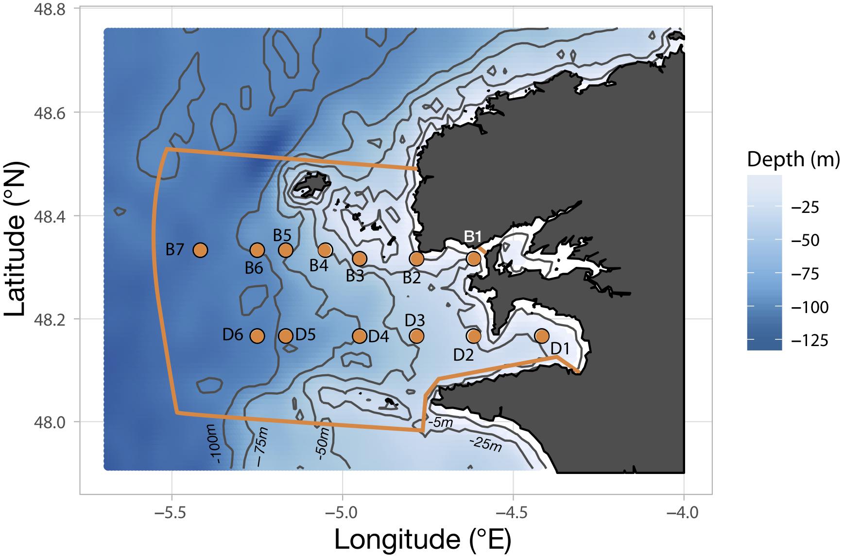
Figure 1. Position of the sampling stations constituting the two transects B and D along the bathymetric gradient of the Iroise Sea. The orange lining delimits the area covered by the “Parc Naturel Marin d’Iroise” (PNMI).

Hydrobiological Data Acquisition

Several abiotic (temperature, salinity, pH, nutrients concentration) and biotic (chlorophyll a concentration, pheophytin a concentration, phytoplankton and mesozooplankton community) variables were measured for each station. Temperature and salinity profiles were measured with a WTW probe (Cond 1970i) equipped with a standard conductivity measuring cell (TetraCon 325/C), from 1 m depth to the stations’ maximum depth. Nutrient concentrations (nitrates, phosphates and silicates), pH, chlorophyll a concentration ([Chl-a]) and pheophytin a concentration ([Pheo-a]) were measured by the LABOCEA laboratory¹ from water samples collected with a 5 L Niskin bottle at the subsurface (approximately 1 m depth). Sampling and in laboratory measurements followed the standard protocols of the Service d’Observation en Milieu LITtoral (SOMLIT²). In addition, the difference between the subsurface temperature (Ts) and the bottom temperature (Tb) was used as an index of water column stratification (ΔT). A ΔT value superior to 1.5°C is a reasonable index for a stratified water column (Schultes et al., 2013). The stations sampled as well as the measured variables are summarized in the Supplementary Table S1.

Satellite Data Acquisition

To assess how in situ measurements compare to the natural temporal variability of temperature and [Chl-a] over the period of interest (2011–2015), satellite sea surface temperature (SST) and surface chlorophyll a concentration ([Chl-a]_sat) were retrieved³. For SST, the 8 day composites Aqua MODIS-derived 11 μm wavelength were used, at a 4 km resolution, and extracted for every date comprised between the 01/01/2011 and the 12/30/2015, within a spatial box encompassing the region of interest (–6.0 < longitude < –4.0; 48.0 < latitude < 49.0). For [Chl-a]_sat, the 4 km Aqua MODIS-derived L3SMI 8 day composites were extracted, over the same period and following the same spatial box. Quartiles of SST and [Chl-a]_sat were calculated for each date and the obtained time series were plotted to visualize the main modes of temporal variability in the area.

Phytoplankton Sampling and Identification

Seawater samples were collected from the 5 L Niskin bottle and placed into dark 250 ml volume flasks, fixed with Lugol’s solution, and stored at room temperature for microscopy analysis. Subsamples of 50 ml were concentrated using Utermöhl settling chambers (Hasle, 1988) and counting was carried out with an inverted microscope equipped with phase contrast (Wild M40). Enumerations were carried out on diametrical transects using a total magnification of 300 or 600×. Alternatively, the totality of the chamber surface was examined depending on the size and the abundance of the species (Lund et al., 1958). Phytoplankton cells were identified to the lowest possible taxonomic rank: most of the diatoms, dinoflagellates, and nanophytoplankton could be identified to genus and species level except for the coccolithophores (defined as “Emiliana-like”), and the Cryptophyta. Picophytoplankton could not be identified nor measured with the methodology used.

Mesozooplankton Sampling and Identification

Mesozooplankton sampling consisted of vertical hauls from 5 m above the bottom to the surface, carried out with a 200 μm mesh size net (57 cm opening diameter). The net was not fitted with a flow-meter. The filtering efficiency was assumed to be sufficiently good and constant over time therefore the filtered volumes were estimated by multiplying the net’s mouth opening surface by the length of cable rolled out during each deployment. Zooplankton samples were immediately preserved on board with 4% sodium tetraborate buffered formaldehyde. A total of 131 samples were collected. The samples were digitized using the Zooscan at the Villefranche Platform for Quantitative imaging (Gorsky et al., 2010). The Zooscan is a waterproof flatbed scanner that generates 16 bit gray-level high resolution images of zooplankton samples. Each of the samples collected was first divided into two size fractions using 1000 μm sieves: d1 for the organisms larger than 1 mm and d2 for the organisms smaller than 1 mm. Each of the two size fractions (d1, d2) was aliquoted with a Motoda plankton splitter to reach aliquots containing nearly 500 to 1000 objects, and imaged with the Zooscan. The initial size fractionation was intended to limit the under-representation of large objects that would become rare after aliquoting the whole sample at once. Image analysis was done on all images using Zooprocess. Images were segmented to spot the objects, and Zooprocess enabled the measurements of 42 features associated with each object, including morphological features (i.e., area of the objects, major and minor axes of ellipsoid that best fit the object, fractal dimension of the objects outlines, etc.) and gray level features (i.e., mean, minimum and maximum values, skewness and kurtosis of gray level distributions, etc.). The measured features were used to perform automatic identification of digitized objects. Automatic identification of objects was done using EcoTaxa⁴. A supervised machine-learning algorithm was used to classify all objects (Random Forest; Breiman, 2001). They were all thoroughly visually inspected thereafter to provide a sorting in nearly 70 biological categories (excluding detritus, bubbles and other scanning artifacts).

Analyses

Phytoplankton Community Structure

Phytoplankton counts were first aggregated into three functional groups of wide taxonomic range that can be used to depict phytoplankton size structure: diatoms, dinoflagellates and nanoflagellates. Correspondence Analysis (CA; Legendre and Legendre, 2012) was performed on the resulting phytoplankton abundances without any prior transformation. CA is an ordination technique that allows description of community structure from contingency tables with frequency-like data that are dimensionally homogeneous (i.e., abundances derived from counts, with integers and zeros). In the CA, relationships between rows (i.e., sampling stations) and columns (i.e., phytoplankton counts) were quantified with the χ² distance (Legendre and Legendre, 2012). To assess the seasonal variations in phytoplankton structure, a bivariate plot was made using the coordinates of the stations on the first two principal components of the CA (CA1 and CA2) and by highlighting the season during which the station was sampled (spring, summer or fall). The station scores along CA1 were then used as a Phytoplankton Community Index (PCI) that summarized phytoplankton community and size structure. In addition, non-parametric variance analyses were used to test the potential seasonal and inter-annual variations in phytoplankton total, and per-group, abundances. Linear regressions between abundances and longitude were performed to test the strength of the coast-open sea gradient.

Species and genus-level phytoplankton counts (cells/mL) were then used to examine finer phytoplankton community structure and its environmental covariates through a Canonical Correspondence Analysis (CCA; Ter Braak, 1986). The CCA is an extension of the CA (i.e., distances between objects are based on the χ² distance) that adds linear regressions between the canonical axes and external environmental variables to further constrain the ordination of sampling stations (Ter Braak, 1986). It produces a diagram that illustrates both variations in community composition that are best explained by combinations of environmental predictors and the centroids of the taxa’s distribution along the canonical axes. The chosen environmental variables were the in situ measurements of temperatures (Ts and ΔT), nutrients concentrations (nitrates and silicates), [Chl-a], [Pheo-a], and station maximal depth which embodies the distance to coast gradient. Most of the 70 phytoplankton taxa identified in the samples present low cell counts and tremendous variability at all scales (transect, seasonal or inter-annual), so we restricted the list of taxa to those presenting at least 50000 cell counts in total to focus on the ecologically important groups.

Mesozooplankton Community Structure

The abundances (ind/m³) of each mesozooplankton category were calculated at every sampling station using the number of validated vignettes corrected for the scanned fraction. All “children categories” were taken into account when calculating the abundance of a category (e.g., calanoid abundances included all objects belonging to calanoid families and the objects belonging to the unidentified Calanoïda). Only the 26 most abundant mesozooplankton categories were kept to avoid rare categories biasing the subsequent analysis of community structure (see below), while keeping the taxa that most adequately represent the diversity of the area studied. The 26 groups retained represented about 97% of the total abundance of metazoans in all samples. Therefore, it is unlikely that a group displaying any pattern of significant biological interest was left out from our analyses. The mesozooplankton abundances were combined with the in situ measurements of temperatures (Ts and ΔT), nutrients concentrations (nitrates and silicates), [Chl-a], [Pheo-a], station maximal depth, as well as the PCI derived from the phytoplankton community analysis, for each sampling station.

Canonical redundancy analysis (RDA) was performed to analyze how the selected environmental variables structure mesozooplankton communities. RDA corresponds to the extension of multiple regression analysis applied to multivariate data (Legendre and Legendre, 2012). The Hellinger-transformed mesozooplankton abundances were used as response variables in the RDA and the abovementioned environmental parameters were used as explanatory variables. Hellinger transformation was applied to make the data suitable for a linear method such as the RDA (Legendre and Gallagher, 2001). The explanatory power of the RDA was assessed through its percentage of explained constrained variance (adjusted R²) and its significance was tested with one-way variance analysis (ANOVA) and permutation tests. Like the CA, a bivariate plot was created from the coordinates along the two first RDA principal components and the seasons were highlighted on the bivariate plot. Non-parametric variance analyses (Kruskal and Wallis, 1952) were performed to assess whether mesozooplankton groups exhibit significant seasonal and inter-annual variations of abundances. The same was done for total mesozooplankton after summing the abundances of all categories. Samples from 2012 were not taken into account when testing inter-annual variations since 2012 was sampled in May only. Linear regressions were performed between abundances and longitude to test if mesozooplankton categories, and total mesozooplankton, display coast-offshore gradients.

Copepod Size Ratio

In addition, the imaging technique enabled estimating the size of each organism (Vandromme et al., 2012). Size was measured as the length of the major axis of the ellipsoid that best fits the silhouette of the organism (the “major” feature measured by Zooprocess; Gorsky et al., 2010). Temporal variations of copepod size structure were analyzed through calculation of a size ratio. The copepod size ratio was calculated for each station as the ratio between the abundance of copepods smaller or equal to 1 mm and the abundance of those strictly larger than 1 mm. The 1 mm threshold has been found to effectively discriminate the small from the large copepods across different oceans (Turner, 2004; Razouls et al., 2005-2018). The higher the size ratio, the higher the proportion of small copepods compared to large ones. The potential environmental drivers of the copepod size ratio were explored by calculating pair-wise Spearman rank correlation coefficients (ρ) between the size ratio and the environmental variables used for the abovementioned CCA and the RDA. To evaluate how the relatively low frequency of the sampling cruises in the PNMI (Supplementary Table S1) may affect our results, we examined an additional time series of mesozooplankton sampling that was carried out in 2013 at station D1 (Figure 1), from the 07/01/2013 (d/m/y) to the 10/12/2013 (15 stations in total). Mesozooplankton sampling and identification followed the same protocol as described above. The copepod size ratio was computed for each station and its temporal variability was compared to the one observed from the seasonal sampling cruises.

All analyses were performed with R version 3.4.0 (R Core Team, 2017). The vegan (Oksanen et al., 2013) and FactoMineR (Lê et al., 2008) packages were used for the community analyses. The pastecs package (Grosjean et al., 2014) was used to perform the time series analyses.

Results

SST and [Chl-a]_sat Time Series

Both SST and [Chl-a]_sat displayed seasonal and inter-annual variability (Figure 2). The SST time series (Figure 2A) showed a typical increase in temperature from winter to summer, with maximal temperatures reached in late July or August (i.e., when the median SST > 18°C). Minimal SST values occurred in February and early March, except in 2015 when the minimum value was found in late November. SST displayed some inter-annual variability in the spring warming rates and the timing of the maximum temperature. On average, summer and fall temperatures were higher in 2013 and 2014 than for the other years. Spring warming rates (derived from the slopes of linear regressions between SST and time, from the first week of April and the first week of August) were higher in 2013, 2014, and 2015 (nearly 0.07°C/day) than in 2011 and 2012 (0.04 and 0.05°C/day, respectively).

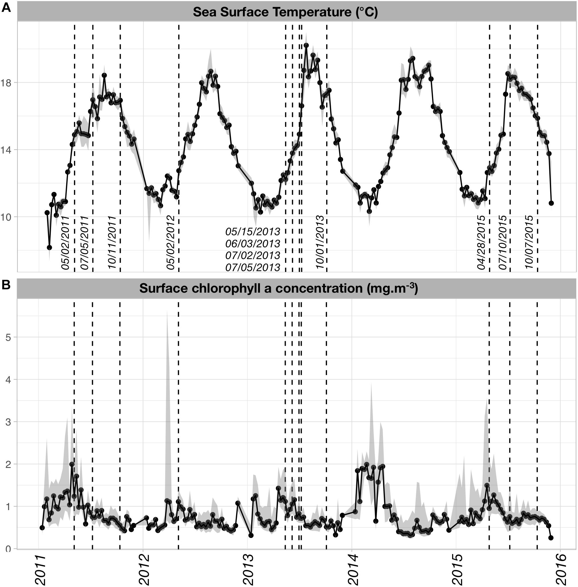
Figure 2. (A) Sea Surface Temperature (SST; °C) and (B) surface chlorophyll a concentration ([Chl-a]_sat; mg m^-3) time series over the time period of our study. SST and [Chl-a]_sat data were obtained from the Aqua MODIS-derived L3SMI 8 day composites (http://coastwatch.pfeg.noaa.gov/erddap/griddap/index.html?page=1&itemsPerPage=1000) that were retrieved over a spatial box encompassing the region of interest (–6.0°E < longitude < –4.0°E; 48.0°N < latitude < 49.0°N). The dates closest to timing of the actual sampling cruises were superimposed on the time series to assess which phases of the natural SST and [Chl-a]_sat cycles were sampled.

The main mode of [Chl-a]_sat variability is a spring increase occurring every year with varying intensity (Figure 2B). The highest [Chl-a]_sat was found in April–May 2014, followed by April 2011 and April–May 2015. In 2012, the highest median [Chl-a]_sat values were found in May but were seldom higher than 1.0 mg m^-3, which made it the least productive year of the series. It was followed by year 2013 which exhibits median [Chl-a]_sat values that are lower than 1.5 mg m^-3.

Apart from 2012, the PNMI cruises sampled the plankton at different phases of the seasonal mode (Figure 2). In 2011, sampling occurred right before and after the warmest conditions, the SST increase in spring was sampled but not the cooling that started late September. However, the temporal decrease of [Chl-a]_sat was sampled for that same year. In 2013, the spring and summer communities were sampled in four successive cruises, all of them taking place before the maximum SST of late July. The September 2013 cruise sampled the Iroise Sea during the cooling phase. Regarding [Chl-a]_sat, the 2013 cruises sampled conditions of decreasing phytoplankton biomass. Very different environmental conditions were sampled for the year 2015, from the colder and productive phase in late April, to the warmer and less productive regimes of July and October, with the latter being in the cooling phase of the SST cycle.

Nano- and Microphytoplankton Community Structure

Phytoplankton community structure at the different stations was characterized by the relative contributions of the three phytoplankton groups (Figure 3). The first CA axis (CA1) summarizes more than 83% of the total variance in phytoplankton abundances and represents a clear gradient in community structure: stations with positive CA1 scores characterized by higher abundances of diatoms than the ones with negative CA1 scores which are dominated by nanoflagellates. CA2 explains nearly all of the remaining 17% of variance and represents the importance of the relative contribution of dinoflagellates. Stations with positive CA2 scores are characterized by higher dinoflagellates abundances.

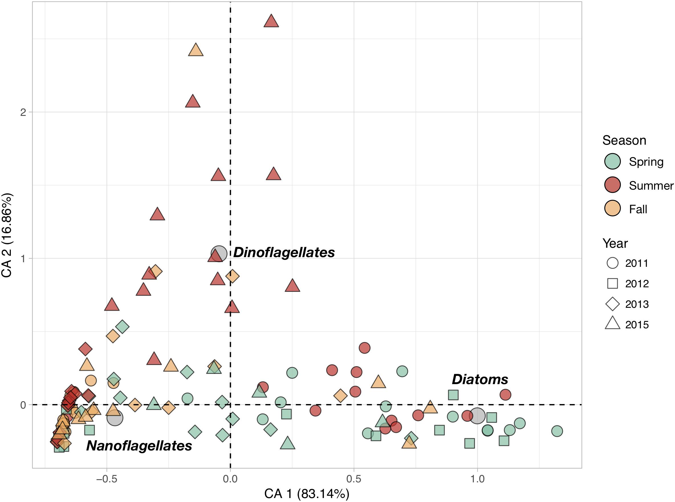
Figure 3. Correspondence Analysis (CA) based on the cell counts of the three main phytoplankton groups (Diatoms, Dinoflagellates and Nanoflagellates). The color of the symbols corresponding to sampling stations (objects) were set according to sampling season (Spring, Summer and Fall), while their shape was changed as a function of the sampling year (2011, 2012, 2013, and 2015) to evidence the seasonal and inter-annual variations. Gray circles represent the position of the scoring variables (phytoplankton groups) in the reduced space.

Phytoplankton communities exhibited clear seasonal patterns. Indeed, most of the spring stations are characterized by higher concentrations of diatoms while the communities sampled in fall are dominated by nanoflagellates. Summer communities showed very strong inter-annual variability: communities from summer 2011 were diatom-rich, whereas those from 2013 were dominated by nanoflagellates, and those from 2015 had relatively high dinoflagellate abundances. Total phytoplankton abundances, as well as diatoms and nanoflagellates abundances, showed significant inter-annual variations in spite of their high variability (Table 1). In total, fewer phytoplankton cells were found in 2015 than in 2011. Diatom abundances were much higher in 2011 than in 2013 and 2015. Significant seasonal variations were found for diatoms and dinoflagellates only. The former were more abundant in spring whereas the latter more abundant in summer. None of the large phytoplankton groups exhibited significant coastal-offshore gradients.

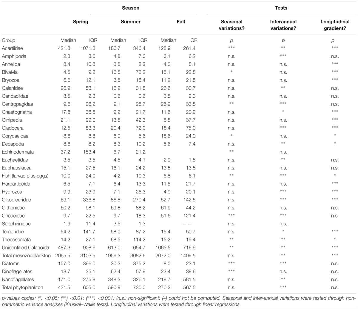
Table 1. Seasonal, inter-annual and longitudinal variations of the median and interquartile ranges (IQR) of the abundance of mesozooplankton and phytoplankton groups.

More detailed taxonomic identification of the phytoplankton allowed linkage of the community composition of each sampling station to the main environmental variables (Figure 4). The retained environmental predictors, and phytoplankton groups, effectively ordinate the stations as the two first components of the CCA, explaining 70.1% of the constrained variance. CCA 1 separates the samples characterized by higher nutrients concentrations from conditions of higher thermal stratification. CCA 2 separates the spring samples of lower temperatures but higher [Chl-a] and [Pheo-a] from the summer and fall samples which show higher surface temperatures. The total depth at the sampling station does not contribute strongly to their ordination in the CCA space, suggesting it does not contribute strongly to shaping changes in generic composition. The strong seasonal pattern in community composition was again apparent. Spring samples were largely dominated by higher concentrations of large colonial diatoms (Guinardia, Skeletonema, Chaetoceros, Cerataulina pelagica). Meanwhile, summer samples showed increased contribution from dinoflagellates (mainly Lepidodinium chlorophorum, Gymnodinium or Heterocapsa), though some samples had strong diatom contributions from Pseudo-nitzschia, Leptocylindrus and Proboscia, as seen from the inter-annual variations in dinoflagellate contributions in the CA (Figure 3). In fall, phytoplankton communities were dominated by smaller nanoflagellates (Prasinophyta, Primnesiophyta and Cryptophyta).

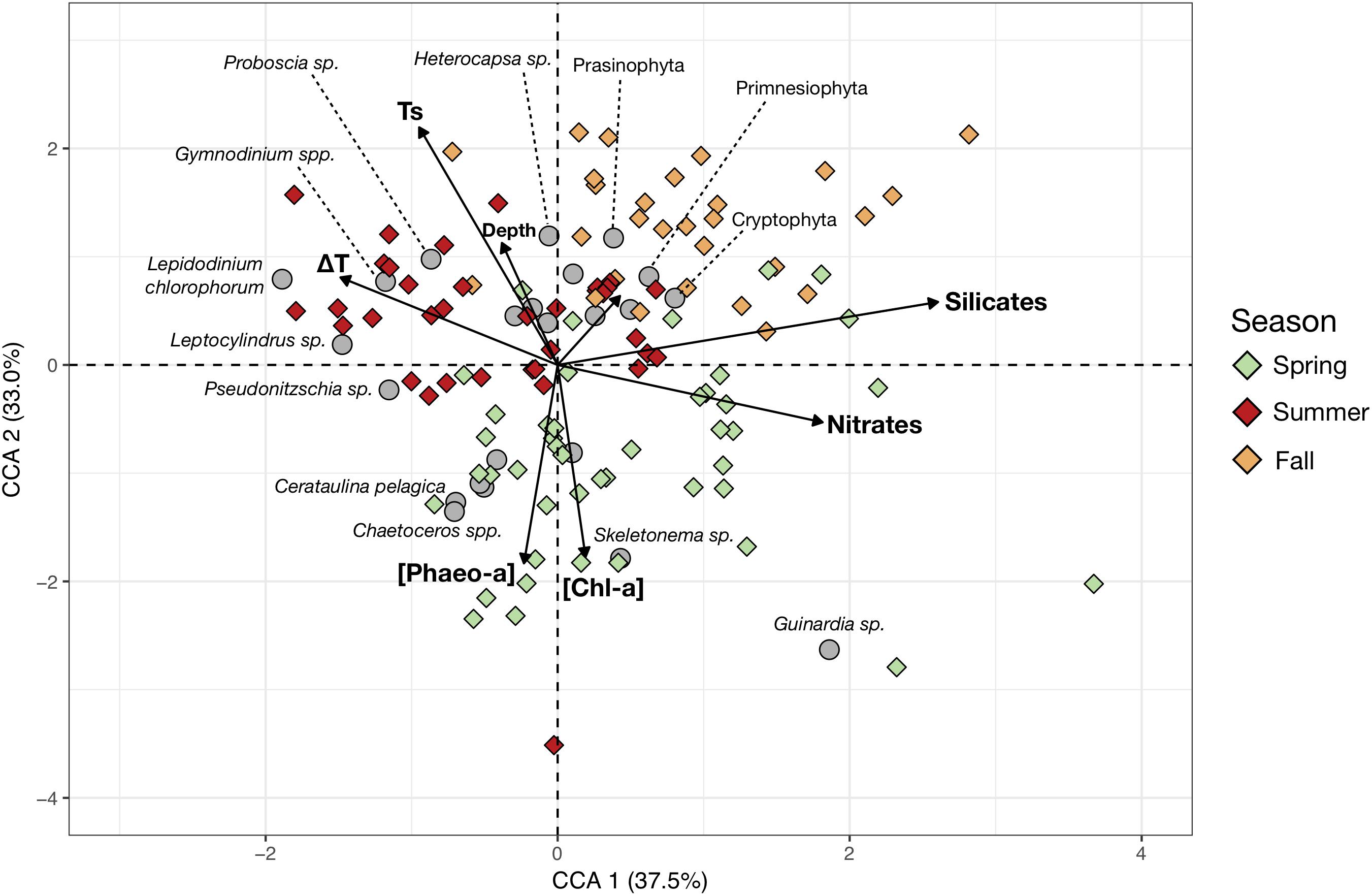
Figure 4. Canonical Correspondence Analysis (CCA) based on the cells counts (cells/mL) of the main phytoplankton species and genera (response variables) and the measured hydrobiological data (explanatory variables, arrows). The color of the symbols corresponding to sampling stations (objects) were colored according to sampling season (Spring, Summer, and Fall). Gray circles represent the mean position of the phytoplankton taxa in the reduced space and therefore indicate the main contributors to the stations community composition. The shortest and unlabelled arrow represents the contribution of phosphate concentrations to ordination of the sampling stations.

Mesozooplankton Abundance

The median and the interquartile ranges of mesozooplankton abundance are summarized in Table 1 together with the significance of their longitudinal, seasonal and inter-annual variations. The median total mesozooplankton abundance was 1956, 2065.5, and 2072.0 ind m^-3 in spring, summer, and fall, respectively. The main mode of mesozooplankton abundance variability was a significant coastal-offshore decrease. None of the mesozooplankton groups studied showed a significant increase of abundance from the coast to the open ocean. Total mesozooplankton abundances also exhibited inter-annual variability, with 2011 presenting higher abundances than 2015.

The two most abundant mesozooplankton groups were the unidentified Calanoïda and the Acartiidae. Other groups of relatively high abundances were appendicularians (Oikopleuridae family), Oithonidae, Temoridae, Calanidae, echinoderms, cirripeds, chaetognaths and euphausiids. Seasonal variations in abundances were significant for four copepod families (Acartiidae, Centropagidae, Corycaeidae and Oncaeidae), together with the unidentified Calanoïda, the pteropods (Thecosomata), fish larvae and eggs, and bivalve larvae. Among those groups, acartiids and fishes were more abundant in spring while pteropods had increased abundances in summer and the remaining groups were more abundant in fall. Groups showing significant inter-annual variations were more numerous. Nine groups showed decreasing abundances from 2011 to 2015: the unidentified Calanoida, acartiids, amphipods, calanids, cladocerans, appendicularians, fish larvae and eggs, pteropods and hydrozoans. Four exhibited a decrease in abundances from 2011 to 2013 followed by an increase 2015: centropagids, chaetognaths, decapods and oncaeids. The abundance of copepods belonging to the Euchaetidae increases from 2011 to 2013. Additionally, 16 groups exhibited a longitudinal gradient of decreasing abundances from the coastal stations to the offshore ones.

Mesozooplankton Community Structure

Mesozooplankton abundances were combined with environmental variables and the PCI derived from phytoplankton counts to identify drivers of mesozooplankton community structure using a RDA (Figure 5). The RDA uses eight variables that significantly constrain the overall variance in mesozooplankton abundances (R² = 0.33; p-value < 0.001). The first two RDA canonical axes (RDA1 and RDA2) explain 61.9 and 19.2% of the total constrained variance, respectively. RDA1 is mainly scored by maximal depth, silicates concentration, PCI, and [Chl-a] and [Pheo-a] to a lesser extent. RDA2 is mainly scored by Ts, followed by ΔT and nitrates concentrations.

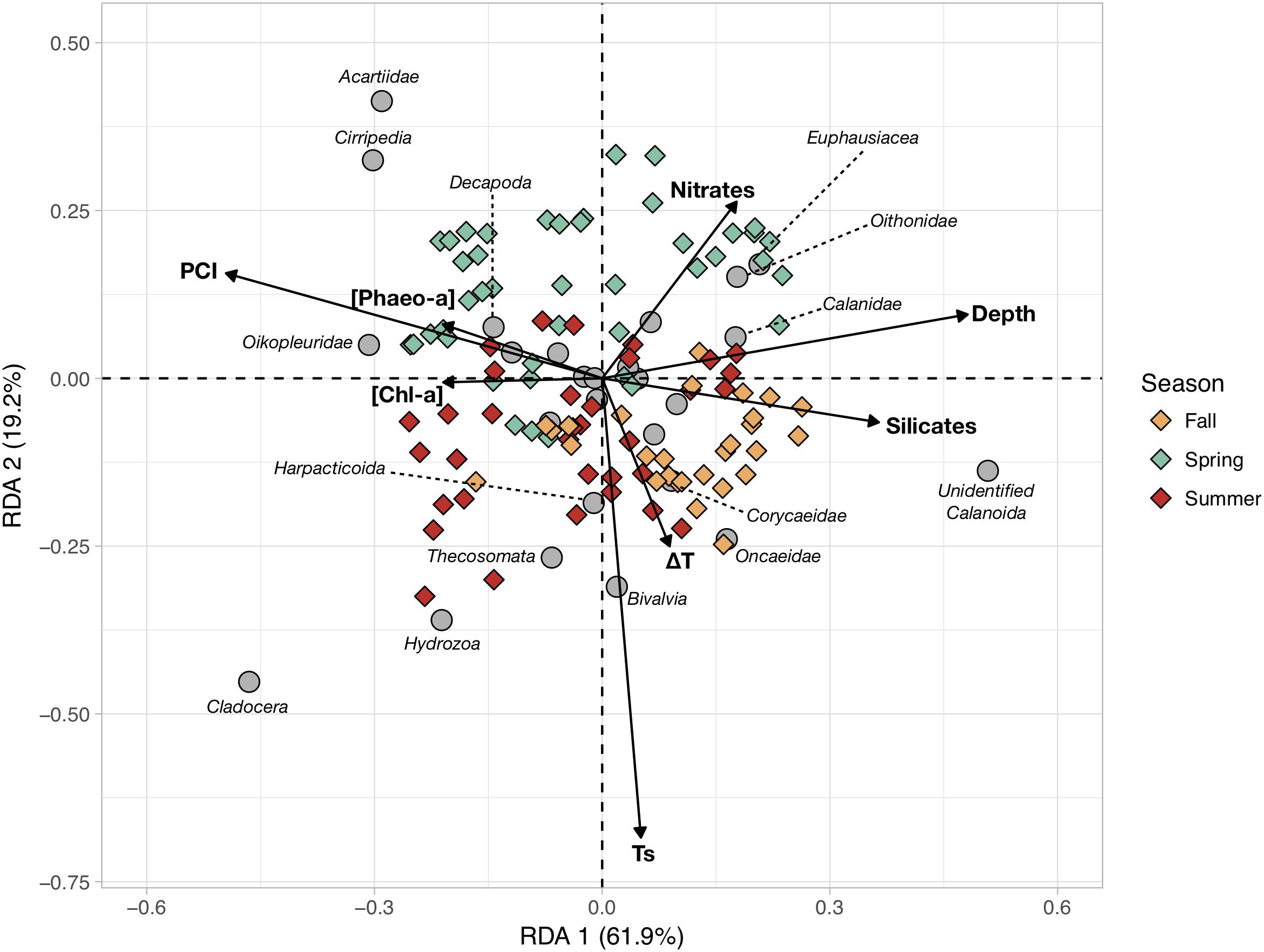
Figure 5. Redundant Discriminant Analysis (RDA) based on the Hellinger-transformed abundances of the main mesozooplankton groups (response variables) and the measured hydrobiological data (explanatory variables, arrows). The color of the symbols corresponding to sampling stations (objects) were colored according to sampling season (Spring, Summer, and Fall).

The stations with positive coordinates along RDA1 were characterized by higher relative abundances of unidentified Calanoïda, euphausiids, oithonids, calanids and oncaeids. In contrast, those groups were less abundant at the stations located on the negative side of RDA1, with higher abundances of cladocerans, appendicularians, cirripeds, acartiids, hydrozoans and decapods. Spring and summer stations were quite scattered across the first canonical axis whereas fall stations mainly showed positive RDA1 scores. Seasonal patterns were clearer along RDA2, as the spring stations were almost all located on the positive side of RDA2 while summer and fall stations were mainly on the negative side, showing warmer and more-stratified water columns. The RDA indicated that the first order of variations of mesozooplankton communities was a coastal-open sea gradient (i.e., east-west depth gradient), with higher diatom abundances and phytoplankton biomass at the stations closer to the coast. The second order mesozooplankton community structure was driven by the seasonal increase in temperature. As shown in Table 1, spring communities are characterized by higher abundances of acartiids, cirripeds, euphausiids, oithonids, appendicularians and decapods. Summer communities present higher abundances of cladocerans, hydrozoans, pteropods, appendicularians, harpacticoids and bivalve larvae. Fall communities show higher contributions of small unidentified Calanoïda and small Poecilostomatoïda (Oncaeidae and Corycaeidae) to a lesser extent.

Variations in Copepod Size Structure

Copepods smaller than 1 mm mainly corresponded to unidentified calanoids and members of the following families: Acartiidae, Oithonidae, Oncaeidae, Temoridae and Corycaeidae (Figure 6). Copepods larger than 1 mm also belonged to unidentified calanoids and acartiids, but they mainly corresponded to Calanidae and, to a lesser extent, Centropagidae, Candaciidae, Euchaetidae and Pontellidae (Figure 6).

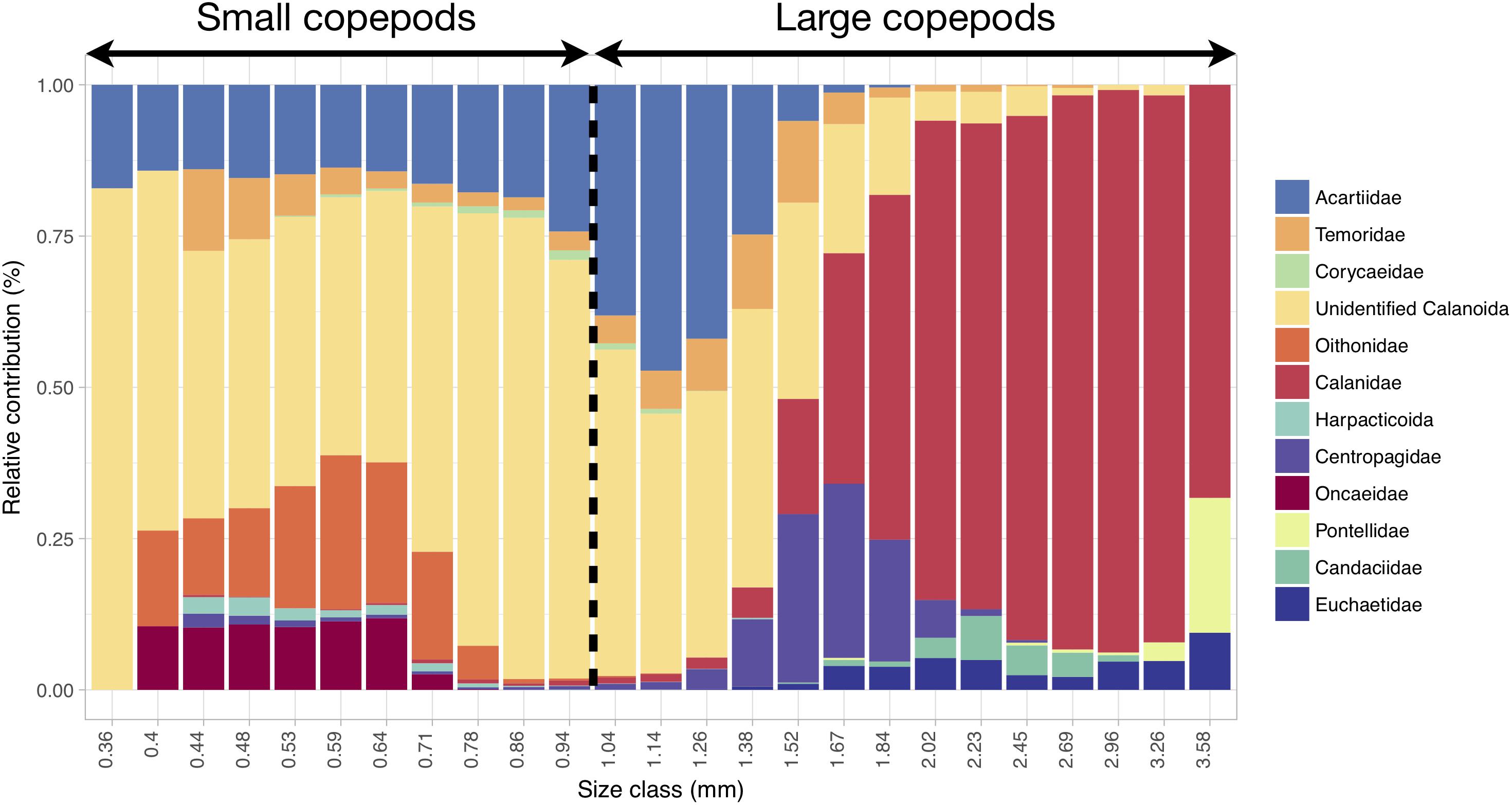
Figure 6. Relative contribution (in % of abundance) of the copepod categories to the size spectrum showing that progressive changes in size correspond to changes in taxonomic composition. The range and categories of the size spectrum were defined based on all copepod images together, and the relative contributions were computed from all samples. The 1 mm threshold chosen for distinguishing small from large copepods is highlighted. Copepod size was estimated through the length of the major axis of the corresponding vignettes.

For each year, the copepod size ratio increased progressively from spring to fall (Figure 7). The strongest seasonal increase occurs in 2015 (Figure 7A). As a result, copepod size ratio varies significantly across seasons (Figure 7B; Kruskal–Wallis tests; p-value < 0.001). The size ratio significantly increased with small copepod abundance (ρ = 0.45; p-value = 1.13 × 10^-6) and decreased with large copepod abundance (ρ = –0.60; p-value = 9.17 × 10^-12).

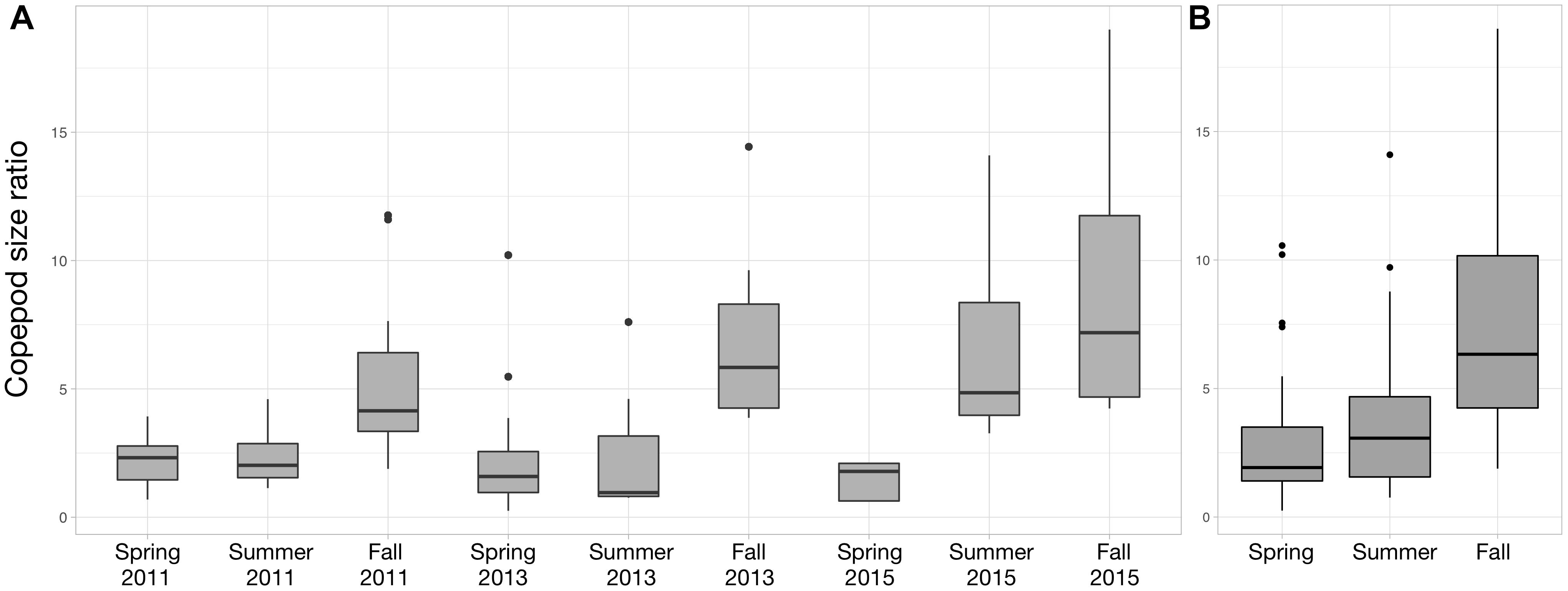
Figure 7. Distribution of the copepod size ratio (small/large) between Spring 2011 and Fall 2015 (A) and between the three seasons (B). Copepod size ratios were computed from the abundances of small (<1 mm) and large (>1 mm) copepods. Data from Spring 2012 were not showed to facilitate the visualization of the seasonal variations (no samples in Summer and Fall 2012), but they were used to compute the variations across the three seasons studied (B).

The rank correlations computed between the copepod size ratio and the environmental variables only revealed significant positive covariations with surface temperature (ρ = 0.31; p-value = 1.17 × 10^-3) and silicates concentration (ρ = 0.31; p-value = 1.41 × 10^-3). The abundance of large copepods increased with the depth of the sampling stations (ρ = 0.49; p-value = 1.28 × 10^-8) and water column stratification (ρ = 0.25; p-value = 9.26 × 10^-3), and decreased with surface temperature (ρ = –0.27; p-value = 4.81 × 10^-3). Meanwhile, the abundance of small copepods increased with the concentration of nitrates (ρ = 0.26; p-value = 8.31 × 10^-3), phosphates (ρ = 0.31; p-value = 1.11 × 10^-3), and silicates (ρ = 0.33; p-value = 6.78 × 10^-4), but decreased with the PCI (ρ = –0.26; p-value = 8.39 × 10^-3). The abundances of small and large copepods showed a significant negative rank correlation (ρ = 0.32; p-value = 8.93 × 10^-4).

Discussion

Changes in Phytoplankton Abundance and Community Structure

Seasonality has a strong impact on both phytoplankton biomass and community structure as evidenced by the [Chl-a]_sat time series (Figure 2B) and the CA based on phytoplankton cell counts (Figure 3). The observed spring bloom dynamics are consistent with earlier studies showing that it is the main mode of variation of phytoplankton biomass in this temperate region (Garcia-Soto and Pingree, 2014). A recent modeling study identified a spring peak in biomass to be the main mode of variation in the annual phytoplankton cycle in the Iroise Sea (Cadier et al., 2017). According to the authors, the spring bloom is triggered by the onset of the seasonal stratification in April-May which creates favorable nutrient and irradiance conditions for large opportunistic diatoms to grow. They also note that phytoplankton can show high concentrations throughout summer thanks to replenishment of nutrients in the coastal waters through a tidal front. These differential dynamics in the physical conditions could explain why the increase in phytoplankton biomass in spring is sometimes harder to differentiate from summer conditions, like in 2012 and 2013, from the satellite data (Figure 2).

Changes in phytoplankton community structure may induce differential bloom timings and intensities. Here, spring blooms are clearly linked to higher contributions of diatoms as this group exhibits significant abundance increases in spring (Table 1 and Figure 3). On the contrary, nanoflagellates remain abundant across all seasons (Table 1). Therefore, seasonal changes in the PCI are driven by seasonal changes in microphytoplankton (diatoms and dinoflagellates) abundance. Such recurrent shifts in the phytoplankton composition and size structure were observed by Cadier et al. (2017). In situ [Chl-a] measurements show higher phytoplankton biomass in spring compared to fall, but not in summer. However, considering the lower temporal coverage of the sampling cruises (three times a year), direct comparison with the [Chl-a]_sat time series should be taken with caution. The observed inter-annual variability of [Chl-a]_sat matches the one described for the Bay of Biscay, with 2013 being way less productive than the previous and following years (Garcia-Soto and Pingree, 2014).

The PCI also showed some inter-annual variability (Figure 3). For instance, 2015 had lower diatom contributions in spring and much higher dinoflagellate contributions in summer. These inter-annual variations could be mediated by species-level resource competition dynamics or small-scale variations of sea currents. The genus and species-level identification of phytoplankton revealed that the diatom spring blooms are mainly composed of large chain-forming genera such as Guinardia, Chaetoceros, Cerataulina pelagica, Skeletonema, and/or Pseudo-nitzschia (Figure 4). Interestingly, the summer samples of 2011 exhibited higher diatom contributions compared to 2013 and 2015 (Figures 3, 4). This was due to relatively higher abundances of other chain-forming diatom genera: Leptocylindrus and Proboscia. Diatom species composition showed inter-annual variability in the Iroise Sea and the observed species bulk is in line with diatom community compositions reported in nearby regions (Hernández-Fariñas et al., 2013; Napoléon et al., 2014; Barnes et al., 2015). Diatom contribution seems to be a key factor in determining mesozooplankton community structure (later discussed in Section “Changes in Copepod Size Structure”) together with maximal depth (reflecting the coastal-offshore gradient) and silicates concentration, as these are the main scoring variables of the first RDA component (Figure 5). Silicates showed a negative correlation with the PCI which is likely due to the consumption of dissolved silica by diatoms as observed during spring blooms (Del Amo et al., 1997). Increased silicate inputs from river runoff linked to more intense precipitations in fall could not explain this pattern because this would lead to higher silicate concentrations near coastal stations, but this is not the case here. In addition, diatom abundances and silica concentration are often negative covariates in the region (Napoléon et al., 2014; Barnes et al., 2015). This observation supports our view that, despite a nutrient limitation of the phytoplankton growth mainly by nitrates after the summer (Del Amo et al., 1997) in very near-shore water, the observed silicate concentrations can be greatly affected by diatom abundance.

Changes in Mesozooplankton Abundance and Community Composition

Ours is the first study to examine the seasonal changes of zooplankton community in the Iroise Sea at the pluri-annual scale. Like for phytoplankton, our findings are generally coherent with previous observations of mesozooplankton community variations in coastal North Atlantic regions. The first-order mode of variations identified here is the coastal-open sea gradient in abundance, which is found for total mesozooplankton and 16 different groups (Table 1). The RDA identifies the coastal-open sea gradient to be the main scoring factor together with the PCI (Figure 5), while changes in [Chl-a] and surface temperature show lower contributions to the percentage of explained constrained variance. The impact of seasonality is more evident when considering RDA1 and RDA2 jointly (Figure 5) or when focusing on copepod size structure (Figure 7). Considering that zooplankton life cycles usually last for months while those of phytoplankton are much shorter (1–3 days), the observed zooplankton community structure is likely to better reflect longer time scales (e.g., seasonality) than phytoplankton.

Using a coast-open sea transect in September 2009 going as far west as 6.3°W, Schultes et al. (2013) analyzed the impact of the frontal features and the strong tidal cycle on plankton production and composition between the end of summer and the beginning of fall. They found the East-West gradient to be the main pattern of plankton abundance variations, except for some groups that peaked at the frontal zone (copepod nauplii and Noctiluca sp.). Our sampling cruises did not extend further than 5.5°W (Figure 1) and our sampling design did not allow us to systematically detect the thermal front because it is characterized by important spatial variations (Le Boyer et al., 2009; Muller et al., 2009). The transects analyzed by Schultes et al. (2013) went beyond 6.3°W, therefore their study covered the full length of the coastal-offshore gradients. Nonetheless, when restricting their results to stations with longitudes comparable to ours, the mesozooplankton abundances estimated here are in the same ranges as those reported by Schultes et al. (2013). Most of the groups that showed a significant decrease of abundance from the coast to the open-ocean in our study overlap with theirs (i.e., Appendicularia, Chaetognatha, Cladocera, Harpacticoida and meroplankton groups such as Cirripedia and Bivalvia) though some discrepancies are also found. For instance, oithonids [Cyclopoida in Schultes et al. (2013)] and calanoids exhibited a strong abundance increase toward offshore waters in Schultes et al. (2013) that is not found in the present data (Table 1). Discrepancies between the two studies may be due to unresolved spatial differences in the mesoscale hydrography, or to the higher temporal coverage of our data spanning different seasons at a pluri-annual scale.

Conversely, some mesozooplankton groups that are known for their coastal affiliations (i.e., bivalve larvae and Harpacticoida) were associated with the temperature (Ts) and the vertical gradient (ΔT) (RDA2; Figure 5) rather than the depth gradient (RDA1), resulting in seasonal patterns that are not visible in Table 1. This is likely due to the non-linear variation of surface temperature from East to West when the external and internal Ushant fronts are established (Le Boyer et al., 2009; Muller et al., 2009). The external Ushant front is the major hydrological feature of the Iroise Sea between the end of May and the end of October (Le Boyer et al., 2009). It is a tide-driven thermal front that sharply separates thermally stratified open waters from the coastal tidally mixed waters. This generates a bimodal thermal gradient as colder tidally mixed waters are separated from the warm and permanently stratified coastal waters (near the B1, B2, D1 and D2 stations; Figure 1) and from the open waters (Le Boyer et al., 2009). In the same way, the water mass of station D1 is separated from the other mixed waters because tidal currents decreased strongly inside this small bay, and the stratification occurred in summer with high temperature values. As a consequence, the RDA sometimes associates very coastal zooplankton groups, such as Harpacticoïda, with offshore ones on the basis of their affinity with warmer temperatures.

The relatively short time span of our time series prevents identification of the drivers of inter-annual variations in zooplankton abundance and composition. We found a decrease in total abundance from 2011 to 2015 (Table 1) that could not be linked to observed environmental variability because of the short length of the time series. Climatic processes such as the North Atlantic Oscillation (NAO) impact plankton community and abundance in the North Atlantic shelf seas by triggering changes in meteorological conditions (Irigoien and Harris, 2003). Yet, the impact of the NAO (from negative phase in 2011, 2013 to positive in 2015, data found at: https://climatedataguide.ucar.edu/climate-data/hurrell-north-atl antic-oscillation-nao-index-station-based) on zooplankton in the PNMI is difficult to discern because of the variety of influencing factors that prevail in coastal areas (freshwater inputs or anthropogenic pollution; Eloire et al., 2010).

Changes in Copepod Size Structure

The dominant mesozooplankton were the small unidentified Calanoïda (Table 1 and Figure 6) which comprise the copepods that could not be attributed to any copepod family because of the image resolution of the Zooscan. Considering the size range of this group (mainly between 0.3 and 1.7 mm; Figure 6), it might be composed of several small calanoid species and copepodites stages of some of the larger species (such as Calanus spp.). In the North-East Atlantic Ocean, small calanoids are mainly represented by Pseudocalanus elongatus and Paracalanus parvus (Beaugrand et al., 2003; Eloire et al., 2010; Reygondeau et al., 2015), two species that do not belong to any of the copepod families identified here but that exhibit similar body lengths ranges (Razouls et al., 2005-2018). Therefore, it is very likely that our cluster of small unidentified Calanoïda is constituted of two species, which are important food items for pelagic fishes (Beaugrand et al., 2003).

Changes in copepod size structure are important to monitor as they can indicate changes in the species ecological traits which translate in regime shifts in the functioning of the pelagic ecosystem (Beaugrand et al., 2010; Barton et al., 2013; Litchman et al., 2013). In the North Atlantic Ocean, plankton community shifts toward more diverse but smaller phytoplankton and copepods have been associated with SST increases that were paralleled by an overall decrease in the ecosystem production and carbon cycling (Beaugrand et al., 2010). Copepod size indices have also been found to effectively explain regime shifts in the recruitment of economically important fishes in offshore (Beaugrand et al., 2003) and shelf waters (Perretti et al., 2017). Consequently, the seasonal patterns in the copepod size ratio we found should reflect adjustments of the zooplankton community to changes in abiotic conditions (i.e., temperature, hydrography) and phytoplankton biomass and composition in the PNMI.

Changes in surface temperatures are known to be the main driver of shifts toward smaller zooplankton organisms at multiple scales (Daufresne et al., 2009; Beaugrand et al., 2010; Chiba et al., 2015). In agreement with these observations, we found a seasonal shift in size structure toward smaller copepods, for each of the year sampled in the PNMI (Figure 7), one that was matched by increase in surface temperature. The mechanisms underlying these changes could not be thoroughly identified from the data at hand. The stronger rank correlation between the size ratio and the large copepods implies that the former is mainly a consequence of the decrease in the abundance of larger copepods rather than the variation in the abundance of small ones. This is supported by the observations from the time series at station D1 which showed that large copepods are clearly more abundant from April to June while small copepods do not exhibit clear temporal seasonal signal throughout 2013 (Supplementary Figure S1). The decrease in large copepod abundance could be triggered by several non-exclusive processes. For instance, warmer temperatures could hinder the growth of larger copepods (Garzke et al., 2015; Horne et al., 2016), as suggested by the significant negative rank correlation between large copepod abundance and surface temperature. Yet, the measured SST rarely exceeds 18°C (Figure 2) so temperatures in the PNMI stay within the optimal growth window for the Calanidae which reach their peak abundances between 13 and 17°C (C. helgolandicus in our case; Bonnet et al., 2005). The decrease in large copepod abundance could be related to the establishment of the Ushant front (Le Boyer et al., 2009), and its subsequent impact on the size structure and the biogeography of the phytoplankton (Cadier et al., 2017). Larger copepods showed higher abundances in more offshore stations as suggested by the significant negative rank correlation between large copepod abundance and depth. Consequently, they are likely to be restricted to the open sea waters west to the Ushant front where nanoflagellates dominate (Figure 5; Cadier et al., 2017) and where large copepods cannot benefit from the phytoplankton biomass characterizing the more coastal tidally mixed waters. Finally, the seasonal change in phytoplankton structure toward the smaller and less lipid-rich nanoflagellates could also explain the decrease in larger copepods, which usually rely on higher energy requirements than smaller copepods to complete their life cycle (Baumgartner and Tarrant, 2017).

Conclusion

Our study is the first to document the seasonal and inter-annual variations of the abundance, composition and size structure of plankton in the MPA of the Iroise Sea, a region of particular interest for its intense hydrographic activity and its high levels of diversity. A strong seasonality was observed for many emerging properties of the plankton community. In spring, large phytoplankton and copepods contribute to plankton composition whereas nanoflagellates and smaller copepods dominate from summer to fall. We also found spatial patterns as phytoplankton biomass (i.e., [Chl-a]) and mesozooplankton abundance increased toward the coast. The copepod size ratio indicated that larger copepods are found at offshore stations, which may be due to the formation of a strong thermal front from May to October. Overall, our observations are coherent with the imprint of seasonality on the plankton of the North Atlantic Ocean (Beaugrand et al., 2010), as the sampled community is part of a wider planktonic biocenosis that is connected throughout the northeastern Atlantic shelves.

Although we could not clearly identify the underlying mechanisms driving the observed patterns, it is very likely that seasonal temperature changes related to atmospheric forcing and the installation of the strong Ushant front greatly contribute to the re-organization of the plankton and its production in the Iroise Sea. Continuing the transects will be crucial to understand the drivers of inter-annual variations in plankton abundance and size structure, and how those influence the functioning of the food web in the MPA. The plankton indicators we provide improve our understanding of the ecosystem dynamics in the Iroise Sea. The indicators can also inform the actors looking to manage and protect the natural marine resources of the PNMI through an ecosystem-based approach. For instance, two of the main objectives of the PNMI are to guarantee a sustainable consumption of marine resources and to support the small local professional fishermen. This is done by documenting the available fish biomass in the MPA and by agreeing on the fishing effort that is adequate with a long-term consumption of this fish biomass. Sardine (Sardina pilchardus) fisheries have long been an important activity in the Iroise Sea but total sardine catches have been declining since 2014 (Figure 8; catch per unit effort calculated and data provided by the PNMI). Total sardine catches show strong seasonal patterns as larger individuals are found in summer in the MPA (Figure 8). Some studies have showed that changes in the plankton size structure toward smaller phytoplankton and copepods favor the abundance of sardines as their fine feeding apparatus effectively selects preys smaller than 580 μm (Van der Lingen et al., 2009). Consequently, the seasonal changes in zooplankton size structure we document here may be relevant to understanding the drivers of sardine dynamics in the Iroise Sea, as they show concomitant variations. To better understand how sardines abundances are influenced by plankton abundance and size structure, we encourage future studies to examine sardine body condition (Brosset et al., 2015) and stomach content (Garrido et al., 2008), by analyzing sardines and plankton collected inside and outside the PNMI.

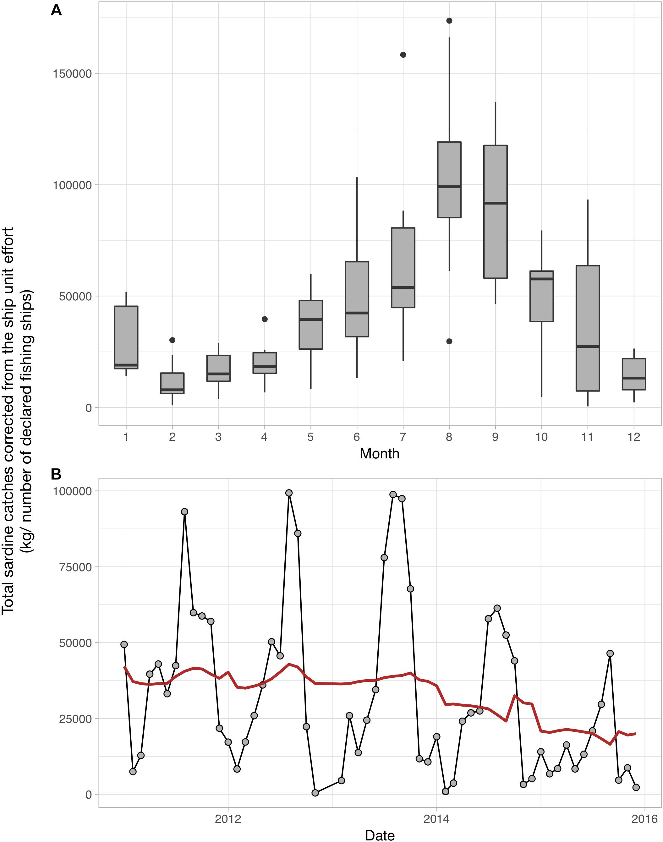
Figure 8. Monthly (A) and inter-annual (B) patterns of Sardina pilchardus catches in the Iroise Sea over the 2011–2016 period. (A) The monthly distribution of S. pilchardus catches corrected by the number of fishing boats. (B) The sum of captured sardines corrected by the number of fishing boats per month over the 2011–2016 period; the red line represents the long term trend in S. pilchardus catches after removing the seasonal variability through a moving average. The sardine catches data were calculated and provided by the PNMI. These data were subsetted from the CPUEs calculated by the PNMI within the framework of fisheries indicators calculation for the “Tableaux de bord” (http://www.parc-marin-iroise.fr/Le-Parc/Objectifs/Tableau-de-bord). They are extracted from the SACROIS data associated to fishing operations carried out in the Iroise Sea, issued from the Fisheries Information System (FIS) of the “Institut Français de Recherche pour l’Exploitation de la Mer” (IFREMER) for the DPMA (Direction of fisheries and aquaculture of the French Ministry of Agriculture and Fisheries). The FIS is an operational and multidisciplinary monitoring network that enables a comprehensive view of fishery systems including their biological, technical, environmental and economical components, including small-scale fisheries. SACROIS is a validation tool for fisheries statistics, aiming to cross-check data from multiple declarative sources. The application crosses information, at the most disaggregated level, from the fishing fleet register, logbooks, monthly declarative forms (for vessels less than 10 m without logbooks, declarative forms adapted to the special features of the small-scale coastal fisheries), sales notes data, VMS data and the scientific census of fishing activity calendar.

Author Contributions

FB, LS, and PP conceptualized the study. LJ, BB, CC, CD, AE, and MP contributed to data curation. FB and LS performed the data analysis. LS and PP supervised the study and acquired the funding. FB and J-OI developed the code for the statistical analyses. FB, LJ, BB, CC, CD, AE, J-OI, FL, MP, and PP contributed to data preparation. FB and LS prepared the original draft. All co-authors proof-read the manuscript prior to submission.

Funding

This work was supported by the European Union’s Horizon 2020 Research and Innovation Program JERICONEXT under the grant agreement no. 654410 and the “Agence Française pour la Biodiversité” (AFB). LS was supported by the CNRS/UPMC Chair VISION. This work was also supported by EMBRC-France, whose French state funds are managed by the ANR within the Investments of the Future program under reference ANR-10-INBS-02.

Conflict of Interest Statement

The authors declare that the research was conducted in the absence of any commercial or financial relationships that could be construed as a potential conflict of interest.

Acknowledgments

We thank the RADEZOO service of the Observatoire Océanographique de Villefranche-sur-Mer (OOV), and particularly Louis Caray-Counil, as well as the crews of the Albert Lucas, the Augustine and the Val Bel for helping with data collection, and the PIQv platform for image analysis (http://rade.obs-vlfr.fr/RadeZoo/). We also thank Dr. Pablo Brosset and Dr. Martin Huret for their comments on an early version of the manuscript, and Dr. John Dolan for revising the language.

Supplementary Material

The Supplementary Material for this article can be found online at: https://www.frontiersin.org/articles/10.3389/fmars.2019.00214/full#supplementary-material

FIGURE S1 | Summary of all the sampling stations performed in the Parc Naturel Marin d’Iroise over the 2011–2015 period (name, date, coordinates, sampling depth, and sampled abiotic and biotic variables).

TABLE S1 | Table summarizing the cell counts (cells/mL) for all the phytoplankton taxa identified to the lowest taxonomic level possible from the sampling cruises carried out in the Parc Naturel Marin d’Iroise.

Footnotes

1. ^ http://www.labocea.fr/
2. ^ http://somlit.epoc.u-bordeaux1.fr/fr/spip.php?article369
3. ^ http://coastwatch.pfeg.noaa.gov/erddap/griddap/index.html?page=1&itemsPerPage=1000
4. ^ http://ecotaxa.obs-vlfr.fr/

References

Barnes, M. K., Tilstone, G. H., Suggett, D. J., Widdicombe, C. E., Bruun, J., Martinez-Vicente, V., et al. (2015). Temporal variability in total, micro-and nano-phytoplankton primary production at a coastalsite in the western English Channel. Prog. Oceanogr. 137, 470–483. doi: 10.1016/j.pocean.2015.04.017
Barton, A. D., Pershing, A. J., Litchman, E., Record, N. R., Edwards, K. F., Finkel, Z. V., et al. (2013). The biogeography of marine plankton traits. Ecol. Lett. 16, 522–534. doi: 10.1111/ele.12063
Baumgartner, M. F., and Tarrant, A. M. (2017). The physiology and ecology of diapause in marinecopepods. Annu. Rev. Mar. Sci. 9, 387–411. doi: 10.1146/annurev-marine-010816-060505
Beaugrand, G., Brander, K. M., Lindley, J. A., Souissi, S., and Reid, P. C. (2003). Plankton effect on codrecruitment in the North Sea. Nature 426, 661–664.
Beaugrand, G., Edwards, M., and Legendre, L. (2010). Marine biodiversity, ecosystem functioning,and carbon cycles. Proc. Natl. Acad. Sci. U.S.A. 107, 10120–10124. doi: 10.1073/pnas.0913855107
Berthou, P., Masse, J., Duhamel, E., Begot, E., Laurans, M., Biseau, A., et al. (2010). La pêcherie de bolinche dans le périmètre du parc naturel marin d’Iroise. PNMI (Parc Naturel Marin d’Iroise), Le Conquet 29, Ref.R.INT.STH/LBH, 22.
Bonnet, D., Richardson, A., Harris, R., Hirst, A., Beaugrand, G., Edwards, M., et al. (2005). An overview of Calanus helgolandicus ecology in European waters. Prog. Oceanogr. 65, 1–53. doi: 10.1016/j.pocean.2005.02.002
Brosset, P., Ménard, F., Fromentin, J. M., Bonhommeau, S., Ulses, C., Bourdeix, J. H., et al. (2015). Influence of environmental variability and age on the body condition of small pelagic fish in the Gulfof Lions. Mar. Ecol. Prog. Ser. 529, 219–231. doi: 10.3354/meps11275
Brucet, S., Boix, D., López-Flores, R., Badosa, A., and Quintana, X. D. (2006). Size and species diversity ofzooplankton communities in fluctuating mediterranean salt marshes. Estuar. Coast. Shelf Sci. 67, 424–432. doi: 10.1016/j.ecss.2005.11.016
Cadier, M., Gorgues, T., Sourisseau, M., Edwards, C. A., Aumont, O., Marié, L., et al. (2017). Assessing spatial and temporal variability of phytoplankton communities’ composition in the Iroise Seaecosystem (Brittany, France): A 3D modeling approach. Part 1: biophysical control over planktonfunctional types succession and distribution. J. Mar. Syst. 165, 47–68. doi: 10.1016/j.jmarsys.2016.09.009
Chiba, S., Batten, S. D., Yoshiki, T., Sasaki, Y., Sasaoka, K., Sugisaki, H., et al. (2015). Temperatureand zooplankton size structure: climate control and basin-scale comparison in the North Pacific. Ecol. Evol. 5, 968–978. doi: 10.1002/ece3.1408
Daufresne, M., Lengfellner, K., and Sommer, U. (2009). Global warming benefits the small in aquaticecosystems. Proc. Natl. Acad. Sci. U.S.A. 106, 12788–12793. doi: 10.1073/pnas.0902080106
Del Amo, Y., Le Pape, O., Tréguer, P., Quéguiner, B., Ménesguen, A., and Aminot, A. (1997). Impacts ofhigh-nitrate freshwater inputs on macrotidal ecosystems. I. Seasonal evolution of nutrient limitation for thediatom-dominated phytoplankton of the Bay of Brest (France). Mar. Ecol. Prog. Ser. 161, 213–224. doi: 10.3354/meps161213
Duhamel, E., Laspougeas, C., and Fry, A. (2011). Rapport Final du Programme D’embarquements à Bord Desbolincheurs Travaillant Dans le Parc Naturel Marin d’Iroise.
Eloire, D., Somerfield, P. J., Conway, D. V., Halsband-Lenk, C., Harris, R., and Bonnet, D. (2010). Temporal variability and community composition of zooplankton at station L4 in the Western channel: 20 years of sampling. J. Plankton Res. 32, 657–679. doi: 10.1093/plankt/fbq009
Frangoudes, K., and Garineaud, C. (2015). “Governability of kelp forest small-scale harvesting in the Iroise Sea, France,” in Interactive Governance for Small-Scale Fisheries: Global Reflections, eds S. Jentoft and R. Chuenpagdee (Cham: Springer International Publishing), 101–115. doi: 10.1007/978-3-319-17034-3_6
Garcia-Soto, C., and Pingree, R. D. (2014). A new look at the oceanography of the Bay of Biscay. Deep Sea Res. Part II Top. Stud. Oceanogr. 106, 1–4. doi: 10.1016/j.dsr2.2014.07.010
Garrido, S., Ben-Hamadou, R., Oliveira, P. B., Cunha, M. E., Chícharo, M. A., and van der Lingen, C. D. (2008). Diet and feeding intensity of sardine Sardina pilchardus: correlation with satellite-derivedchlorophyll data. Mar. Ecol. Prog. Ser. 354, 245–256. doi: 10.3354/meps07201
Garzke, J., Ismar, S. M. H., and Sommer, U. (2015). Climate change affects low trophic level marineconsumers: warming decreases copepod size and abundance. Oecologia 177, 849–860. doi: 10.1007/s00442-014-3130-4
Gattuso, J.-P., Magnan, A., Billé, R., Cheung, W., Howes, E., Joos, F., et al. (2015). Contrasting futuresfor ocean and society from different anthropogenic CO2 emissions scenarios. Science 349:aac4722. doi: 10.1126/science.aac4722
Gill, D. A., Mascia, M. B., Ahmadia, G. N., Glew, L., Lester, S. E., Barnes, M., et al. (2017). Capacityshortfalls hinder the performance of marine protected areas globally. Nature 543:665. doi: 10.1038/nature21708
Gorsky, G., Ohman, M. D., Picheral, M., Gasparini, S., Stemmann, L., Romagnan, J.-B., et al. (2010). Digital zooplankton image analysis using the ZooScan integrated system. J. Plankton Res. 32, 285–303. doi: 10.1093/plankt/fbp124
Grosjean, P., Ibanez, F., and Etienne, M. (2014). Pastecs: Package for Analysis of Space-Time Ecological Series. R Package Version, 1.3–18.
Hasle, G. R. (1988). “The inverted-microscope method,” in Phytoplankton Manual, ed. A. Sournia (Paris: UNESCO), 88–96.
Hernández-Fariñas, T., Soudant, D., Barillé, L., Belin, C., Lefebvre, A., and Bacher, C. (2013). Temporal changes in the phytoplankton community along the French coast of the eastern English Channel and the southern Bight of the North Sea. ICES J. Mar. Sci. 71, 821–833. doi: 10.1093/icesjms/fst192
Horne, C. R., Hirst, A. G., Atkinson, D., Neves, A., and Kiørboe, T. (2016). A global synthesis ofseasonal temperature–size responses in copepods. Glob. Ecol. Biogeogr. 25, 988–999. doi: 10.1111/geb.12460
Huon, M., Jones, E. L., Matthiopoulos, J., McConnell, B., Caurant, F., and Vincent, C. (2015). Habitatselection of gray seals (Halichoerus grypus) in a marine protected area in France. J. Wild Life Manage. 79, 1091–1100. doi: 10.1002/jwmg.929
Irigoien, X., and Harris, R. P. (2003). Interannual variability of Calanus helgolandicus in the English Channel. Fish. Oceanogr. 12, 317–326. doi: 10.1046/j.1365-2419.2003.00247.x
Kruskal, W. H., and Wallis, W. A. (1952). Use of ranks in one-criterion variance analysis. J. Am. Stat. Assoc. 47, 583–621. doi: 10.1080/01621459.1952.10483441
Le Boyer, A., Cambon, G., Daniault, N., Herbette, S., Le Cann, B., Marie, L., et al. (2009). Observations of the Ushant tidal front in September 2007. Continent. Shelf Res. 29, 1026–1037. doi: 10.1016/j.csr.2008.12.020
Legendre, P., and Gallagher, E. D. (2001). Ecologically meaningful transformations for ordination ofspecies data. Oecologia 129, 271–280. doi: 10.1007/s004420100716
Lê, S., Josse, J., and Husson, F. (2008). FactoMineR: an R package for multivariate analysis. J. Stat. Softw. 25, 1–18. doi: 10.18637/jss.v025.i01
Litchman, E., Ohman, M. D., and Kiørboe, T. (2013). Trait-based approaches to zooplanktoncommunities. J. Plankton Res. 35, 473–484. doi: 10.1016/j.marenvres.2017.04.011
Lubchenco, J., and Grorud-Colvert, K. (2015). Making waves: the science and politics of oceanprotection. Science 350, 382–383. doi: 10.1126/science.aad5443
Lund, J., Kipling, C., and Le Cren, E. (1958). The inverted microscope method of estimating algalnumbers and the statistical basis of estimations by counting. Hydrobiologia 11, 143–170. doi: 10.1007/bf00007865
Mariette, V., and Le Cann, B. (1985). Simulation of the formation of Ushant thermal front. Continent. Shelf Res. 4, 637–660. doi: 10.1016/0278-4343(85)90034-2
McClellan, C. M., Brereton, T., Dell’Amico, F., Johns, D. G., Cucknell, A.-C., Patrick, S. C., et al. (2014). Understanding the distribution of marine megafauna in the English Channel region: identifyingkey habitats for conservation within the busiest seaway on earth. PLoS One 9:e89720. doi: 10.1371/journal.pone.0089720
McGinty, N., Johnson, M. P., and Power, A. M. (2014). Spatial mismatch between phytoplanktonand zooplankton biomass at the Celtic Boundary Front. J. Plankton Res. 36:14461460.
McGinty, N., Power, A., and Johnson, M. (2011). Variation among northeast Atlantic regions in theresponses of zooplankton to climate change: not all areas follow the same path. J. Exp. Mar. Biol. Ecol. 400, 120–131. doi: 10.1016/j.jembe.2011.02.013
Muller, H., Blanke, B., Dumas, F., Lekien, F., and Mariette, V. (2009). Estimating the lagrangianresidual circulation in the Iroise Sea. J. Mar. Syst. 78, S17–S36.
Napoléon, C., Fiant, L., Raimbault, V., Riou, P., and Claquin, P. (2014). Dynamics of phytoplanktondiversity structure and primary productivity in the English Channel. Mar. Ecol. Prog. Ser. 505, 49–64. doi: 10.3354/meps10772
Oksanen, J., Blanchet, F. G., Kindt, R., Legendre, P., Minchin, P. R., O’hara, R., et al. (2013). Package ‘vegan’. Community Ecology Package, Version 2(9).
Perretti, C. T., Fogarty, M. J., Friedland, K. D., Hare, J. A., Lucey, S. M., McBride, R. S., et al. (2017). Regime shifts in fish recruitment on the Northeast US Continental Shelf. Mar. Ecol. Prog. Ser. 574, 1–11. doi: 10.3354/meps12183
Pingree, R., Holligan, P., and Mardell, G. (1978). The effects of vertical stability on phytoplanktondistributions in the summer on the northwest European Shelf. Deep Sea Res. 25, 1011–1028. doi: 10.1016/0146-6291(78)90584-2
R Core Team (2017). R: A Language and Environment for Statistical Computing. Vienna: R Foundation for StatisticalComputing.
Razouls, C., de Bovée, F., Kouwenberg, J., and Desreumaux, N. (2005–2018). Diversity and Geographic Distribution of Marine Planktonic Copepods. Paris: Sorbonne Université.
Reygondeau, G., Molinero, J. C., Coombs, S., MacKenzie, B. R., and Bonnet, D. (2015). Progressive changes in the Western English Channel foster a reorganization in the plankton food web. Prog. Oceanogr. 137, 524–532. doi: 10.1016/j.pocean.2015.04.025
Roberts, C. M., Hawkins, J. P., and Gell, F. R. (2005). The role of marine reserves in achievingsustainable fisheries. Philoso. Trans. R. Soc. Lond. B Biol. Sci. 360, 123–132.
Rombouts, I., Beaugrand, G., Artigas, L. F., Dauvin, J.-C., Gevaert, F., Goberville, E., et al. (2013). Evaluating marine ecosystem health: case studies of indicators using direct observations and modellingmethods. Ecol. Ind. 24, 353–365. doi: 10.1016/j.ecolind.2012.07.001
Schultes, S., Sourisseau, M., Le Masson, E., Lunven, M., and Marié, L. (2013). Influence of physicalforcing on mesozooplankton communities at the Ushant tidal front. J. Mar. Syst. 109, 191–202.
Secretariat of the CBD (2011). Aichi Target 11. Decision X/2. Montreal, CA: Secretariat Convention on Biological Diversity.
Stemmann, L., and Boss, E. (2012). Plankton and particle size and packaging: from determining optical properties to driving the biological pump. Annu. Rev. Mar. Sci. 4, 263–290. doi: 10.1146/annurev-marine-120710-100853
Ter Braak, C. J. (1986). Canonical correspondence analysis: a new eigenvector technique formultivariate direct gradient analysis. Ecology 67, 1167–1179. doi: 10.2307/1938672
Turner, J. T. (2004). The importance of small planktonic copepods and their roles in pelagic marinefood webs. Zool. Stud. 43, 255–266.
UNEP-WCMC and IUCN (2016). Protected Planet Report 2016. Gland: International Union for Conservation of Nature.
Van der Lingen, C., Bertrand, A., Bode, A., Brodeur, R., Cubillos, L., Espinoza, P., et al. (2009). Trophic dynamics of small pelagic fish. Center Mar. Environ. Stud. 29:31.
Vandromme, P., Stemmann, L., Garcìa-Comas, C., Berline, L., Sun, X., and Gorsky, G. (2012). Assessing biases in computing size spectra of automatically classified zooplankton from imagingsystems: a case study with the ZooScan integrated system. Methods Oceanogr. 1, 3–21. doi: 10.1016/j.mio.2012.06.001
Witt, M. J., Broderick, A. C., Johns, D. J., Martin, C., Penrose, R., Hoogmoed, M. S., et al. (2007). Prey landscapes help identify potential foraging habitats for leatherback turtles in the NE Atlantic. Mar. Ecol. Prog. Ser. 337, 231–243. doi: 10.3354/meps337231
Keywords: Iroise Sea, plankton, MPA, temporal variability, community composition, size structure
Citation: Benedetti F, Jalabert L, Sourisseau M, Becker B, Cailliau C, Desnos C, Elineau A, Irisson J-O, Lombard F, Picheral M, Stemmann L and Pouline P (2019) The Seasonal and Inter-Annual Fluctuations of Plankton Abundance and Community Structure in a North Atlantic Marine Protected Area. Front. Mar. Sci. 6:214. doi: 10.3389/fmars.2019.00214
Received: 28 September 2018; Accepted: 05 April 2019;
Published: 24 April 2019.
Edited by:
Alberto Basset, University of Salento, ItalyReviewed by:
Jan Marcin Weslawski, Institute of Oceanology (PAN), PolandJohn Kenneth Pearman, Cawthron Institute, New Zealand
Copyright © 2019 Benedetti, Jalabert, Sourisseau, Becker, Cailliau, Desnos, Elineau, Irisson, Lombard, Picheral, Stemmann and Pouline. This is an open-access article distributed under the terms of the Creative Commons Attribution License (CC BY). The use, distribution or reproduction in other forums is permitted, provided the original author(s) and the copyright owner(s) are credited and that the original publication in this journal is cited, in accordance with accepted academic practice. No use, distribution or reproduction is permitted which does not comply with these terms.
*Correspondence: Fabio Benedetti, fabio.benedetti@usys.ethz.ch