Estimating NOX, VOC, and CO variability over India’s 1st smart city: Bhubaneswar

1 Introduction

Volatile organic compounds (VOCs), which are trace elements in the atmosphere, cause serious health issues (Bono et al., 2003). VOCs are also identified as ozone precursors (Khoder, 2007). In most of the VOC studies, a group of aromatic hydrocarbons, known as BTEX (benzene, toluene, ethylbenzene, and xylene) are considered to represent atmospheric VOCs, as they account for ∼40% of the total ambient VOCs (Derwent et al., 2000; Laowagul and Yoshizumi, 2008; Golkhorshidi et al., 2019). The sources for BTEX are widely distributed including fossil fuel combustion, industrial plants, traffic emissions, wood burning, and indoor materials (i.e., industrial paints, adhesives, and degreasing agents) to name a few (Hinwood et al., 2007). The increasing numbers of incineration activities all over the country are also one of the potential anthropogenic sources of BTEX. BTEX analysis is pretty crucial in developing and overpopulated countries like India, as most of the dwellings in urban regions are situated adjacent to high-traffic roads, which acts as main-source regions for BTEX (Masih et al., 2018). The main issue for BTEX measurements comes with low concentration values, which are sometimes close to instrument detection limits (Zalel and Broday, 2008). As the values are very low for BTEX measurements, they have higher uncertainties and are unsuitable for source-apportionment techniques (Paatero and Hopke, 2003; Zalel and Broday, 2008).

Due to low-concentration issues of BTEX, most air quality studies focus on the aerosols, NOX, SOx, and ozone (e.g., Beig et al., 2008; Gogikar et al., 2018; Choudhury et al., 2019; Tyagi et al., 2020); though the concern for BTEX and its related impacts is rapidly increasing. Primary health issues due to BTEX exposure include central nervous system damage and respiratory irritation, and leukemia and carcinogenic diseases are suspected (Zhang et al., 2012). Earlier, air quality issues were restricted only to industrialized cities (Bell and Davis, 2001; Helfand et al., 2001; Managaraj et al., 2022a). Nevertheless, the fast growth of urbanization in conjunction with the population has given rise to severe air pollution problems globally irrespective of local emission sources (Karagulian et al., 2015; Gogikar and Tyagi, 2016; Managaraj et al., 2022b).

In India, BTEX research works are more than a decade old. These studies are not only limited to metropolitan cities such as Delhi (Singh et al., 2010; Sehgal et al., 2011; Singh et al., 2016; Kumar et al., 2017; Garg and Gupta, 2019), Kolkata (Chattopadhyay et al., 1997; Som et al., 2007; Majumder et al., 2009; Majumdar et al., 2011; Majumdar et al., 2012), Chennai (Mohan and Ethirajan, 2012), and Mumbai (Srivastava et al., 2005a; Srivastava et al., 2006; Majumder and Srivastava, 2012) but they were also conducted in other big cities such as Hyderabad (Rekhadevi et al., 2010), Ahmedabad (Sahu and Saxena, 2015; Sahu et al., 2016), Dehradun (Bauri et al., 2016), Kanpur (Bhattacharya and Tangri, 2015), Agra (Singla et al., 2012; Bhardwaj et al., 2017), Firozabad (Chaudhary and Kumar, 2012), Raipur (Dewangan et al., 2013), Darjeeling (Sarkar et al., 2014), and Gorakhpur (Masih et al., 2018).

However, these BTEX studies are mainly focused on North India, with few studies over East India. The only city with a substantial BTEX study in East India is Kolkata (e.g. Chattopadhyay et al., 1997; Som et al., 2007; Majumdar et al., 2011; Majumdar et al., 2012). With increasing population density in other metropolitan cities of eastern India, and due to industrialization and the increasing number of vehicles over the region, it is crucial to understand the nature of BTEX variation in all populated areas, and the relative exposure to people and environments of all major cities. As monitoring and analyzing the exposures will be the first step in understanding the health and environmental impacts of BTEX, the present work analyzed the BTEX variation over Bhubaneswar, the capital city of the state of Odisha, India, for 2 years (2017–2018), where such measurements were made for the first time. This article analyses diurnal and seasonal variations of BTEX with an attempt to correlate the variations with meteorological parameters, and to understand the transported BTEX over the site. We have also developed sector-wise and area-wise emission details for VOC, NOX, and CO over Bhubaneswar to get a detailed understanding of various contributing factors in these pollutants over the city.

2 Site description

The BTEX concentrations were recorded at Utkal University campus located at 20.18°N, 85.50°E, and 45 above MSL in the first smart city of India, Bhubaneswar (Smart CitiesMission, 2017). The sampling site is at a distance of ∼700 m from the nearest national highway (Sahu et al., 2019). Bhubaneswar, the capital city of the state of Odisha, is a tropical station situated in the eastern coastal region of India. The site has the Bay of Bengal from south to east directions with the shortest spatial distance of ∼60 km. (Sahu et al., 2020). Figure 1 depicts the site. The adoption of Bhubaneswar as a smart city implies its further expansion and planned urbanization extending the perimeter of the city, with more greenery and improved quality of life in combination with advanced technological solutions inside the city (Sahu et al., 2020). On the one hand, this technological development will aid the economic growth. Still, on the other hand, all the renovation, construction, and expansion will also alter the levels of air quality for a specific period. The study site has the clear advantage of reporting the BTEX variation over a first-tier smart city of India. For developing the emission scenario of VOC, NOX, and CO, we have accounted for all the possible sources over the whole Bhubaneswar region.

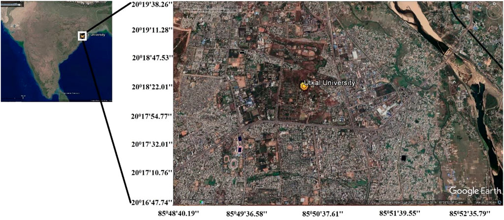
FIGURE 1. Site map of the observational site, with its location on the map of India in the inset. The observational site is represented by a yellow circle in the map, obtained from Google Earth Imagery.

3 Data and methodology

We have utilized hourly data sets of BTEX concentrations with meteorological variables (temperature, humidity, solar radiation, wind speed, and direction) for January 2017–December 2018. The study analyses the BTEX variation to identify the source signatures by analyzing the seasonal, diurnal variations of BTEX concentrations and meteorological parameters with their correlational analysis and studying the ratios of different BTEX components. The study employed the hybrid single-particle Lagrangian integrated trajectories (HYSPLIT) model developed by the National Oceanic and Atmospheric Administration, U.S.A, to calculate the 48-h (2 days) isentropic back trajectories (Yadav et al. (2016); Yadav et al. (2022)). To gain an idea of possible transport regions contributing to the local BTEX emissions at the site, the back trajectories were calculated at three-hour intervals by using Global Data Assimilation System 1° × 1° data sets (Draxler and Hess, 1998).

We have also calculated the total emissions of carbon monoxide (CO) and nitrogen oxides (NOX) over the city in Gg/year over the smart city of Bhubaneswar for the year 2018 for a 1 km × 1 km resolution considering the transportation sector. The calculation has been done by using the top-down approach and by following the methodology of Sahu et al. (2011).

4 Results and discussion

4.1 Variability of meteorological parameters

The seasonal and diurnal variations of the meteorological variables have been studied during the observation period. Table 1 presents the monthly mean values of the meteorological parameters. The site experienced high-summer temperatures of ∼22°C–42°C during the months of May and June, while temperatures during winter months (December–February) were mild in the range of ∼10°C–32°C. The high values of solar radiation, of the order of 144–182 W/m², with a maximum value of ∼770 W/m² were observed in the pre-monsoon season (March–May), whereas low values 77–115 W/m² with a maximum value of the order of ∼590 W/m² were observed during the winter season. The negative minimum SR stands for the night-time SR values, which indicate total outgoing long-wave radiation and the absence of incoming shortwave radiation. The relative humidity is high throughout the year (∼from 64 %–85 %, and maximum values reaching >94 % every month). However, by considering average values, higher values (∼85 %) of humidity were observed in the monsoon season (June–September) where relatively low average values of temperature (∼28°C) were observed. The humidity shows an inverse relation to temperature and solar radiation. The correlation coefficient between temperature and humidity is −0.41 and solar radiation and humidity is −0.66.

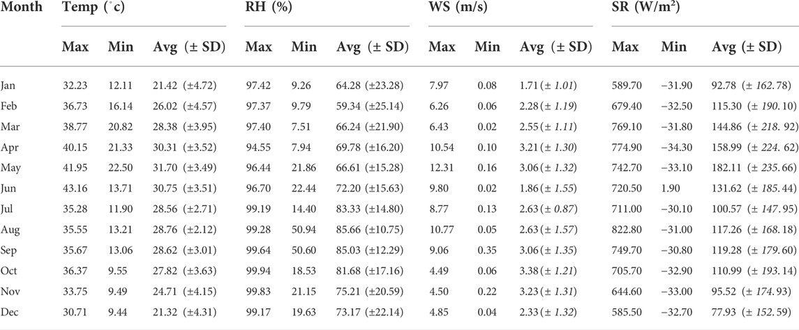
TABLE 1. Mean monthly maximum, minimum, and average (±Standard deviation) values of air temperature, relative humidity, wind speed, and solar radiation for the period of study.

As wind plays a significant role in the transportation and dispersion of any pollutant, it is vital to know the wind patterns at the sampling site. It has been observed that the pre-dominant wind direction was south-easterly at the sampling site throughout the observation period, irrespective of the seasons. We have plotted seasonal wind roses at the observational site, shown in Figure 2. In the winter, winds in the range of 3.6–5.7 m/s blew only from the south-east direction. Although higher winds also blew from the other directions to the site, their duration was very less. Comparatively low winds (<3.6 m/s) blew from all the directions except the north-west. In the pre-monsoon season, winds in the range of 2.1–3.6 m/s blew from all the directions. On the other hand, winds in the range of 3.6–5.7 m/s blew for a longer period from north-east directions and relatively less in other directions. Likewise, higher wind speeds (>5.6 m/s) blew mostly from the north-east directions. For monsoon and post-monsoon seasons, the dominant winds were in the range of 3.6–5.7 m/s, blowing from the south-east direction.

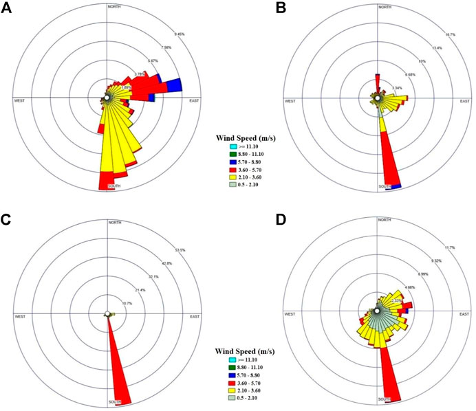
FIGURE 2. Seasonal variations of benzene, toluene, ethyl benzene, m,p-xylene, and o-xylene for (A) pre-monsoon, (B) monsoon, (C) post-monsoon, and (D) winter season.

Sector-wise seasonal wind analysis has also been done and presented in Table 2. It is observed that during all the seasons, the south-easterly sector was dominant with maximum counts of occurrences. However, if we talk about the concentrations of BTEX components, seasonally, the different directions show higher values. For the pre-monsoon season, highest concentrations were for the north-west sector for benzene (B) and toluene (T), whereas the ethyl benzene (EB) and m,p-xylene (m,p-X) did not show significant variations in concentrations. However, the o-xylene (o-X) concentrations were highest for the north-east sector and decreased toward the north-west sector. During the monsoon season, the concentrations of all BTEX components were highest for the north-east sector, followed by the north-west sector. After the south-east sector, more points were recorded in the north-east sector only. However, during the post-monsoon season, the south-west sector was the second-most dominant sector for number of points. The highest concentrations of all the BTEX components in the post-monsoon season were recorded in the north-east sector only. The winter season showed a slight change in the concentration sectors, with the north-east sector showing highest concentrations of B, EB, m,p-X, and o-X but the north-west sector recording the highest concentrations of T. The south-west sector was the second-most dominant sector after the south-east sector for the observational counts in the winter season.

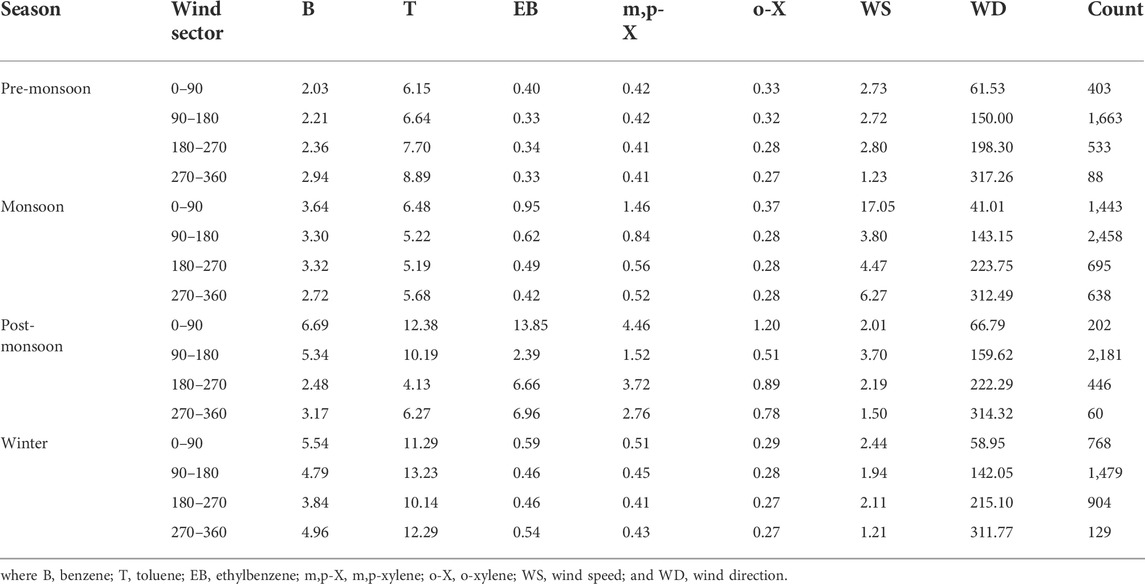
TABLE 2. Seasonal mean concentrations of BTEX components, wind speed, and direction in the four directional sectors of wind.

The monthly variation of meteorological parameters also indicates the land–sea breeze occurrence over the site, which did not allow the temperature to drop down or rise drastically over the region (as visible in the average temperatures of Table 1). The same conclusion can be drawn for the diurnal variations, where the meteorological variables follow a similar pattern (not shown here).

4.2 Benzene, toluene, ethyl benzene, and xylene ratios

The BTEX ratios give us information about the samples responsible for BTEX emission (urban, traffic, fuel, and biomass burning) and also helps in determining the photochemical age of the air parcels. In the present work, BTEX ratios are discussed from the mean BTEX concentrations for the observation period as follows.

4.2.1 m,p-xylene/ethyl benzene

Nelson and Quigley (1983) were among the first to use this ratio to estimate the hydrocarbon age in the atmosphere. The lifetime of m-X and p-X are 11.8 and 19.4 h, whereas the EB has a lifetime of 1.6 days (Monod et al., 2001; Miri et al., 2016; Hamid et al., 2019; da Silva et al., 2020). The ratio will vary from 2.8 to 4.6 if the emission sources are vehicle exhaust (including traffic), solvent petrol, and fuel evaporation (Olson et al., 1992; Jemma et al., 1995), indicating the sources responsible for emission are available near the sampling site. The m,p-xylene/ethyl benzene (m,p-X/EB) ratio for the present study came out as 0.87, which suggests that the m,p-X/EB ratio is not influenced by local traffic emissions (Zweidinger et al., 1988; Monod et al., 2001; da Silva et al., 2020). The results indicate that the usual traffic is now following the stringent pollution control rules and vehicular emissions are under control over the region. The potential sources may be located far from the urban site or sources from the industrial belt.

4.2.2 Toluene/ethyl benzene

Both T and EB are relatively stable hydrocarbons with their atmospheric lifetimes (toward OH radicals) as 1.9 and 1.6 days, respectively (Garzón et al., 2015). The toluene/ethylbenzene (T/EB) ratio came out as 8.23 for the present study. The higher ratio ranging between 8.27 and 9.41 suggests that the samples responsible for emission might be from biomass burning in an urban atmosphere (Monod et al., 2001; Miri et al., 2016). It was identified during a primary field survey that coal and wood were widely being used across hotels and slums in Bhubaneswar, which could be potential sources of BTEX.

4.2.3 Benzene/ethylbenzene

The benzene/ethylbenzene (B/EB) ratio was high at the sampling site (3.86), which suggests that B concentrations were dominant as compared to the EB concentrations. Since B is ubiquitous in urban air (Monod et al., 2001; Hamid et al., 2019; da Silva et al., 2020) with a longer lifetime (∼9.4 days), there is a high chance that the urban air samples accountable for BTEX emissions may be a result of transported emissions from nearby industrial belts.

4.2.4 Toluene/benzene

Architectural surface coatings, industrial solvents, and chemical feedstock are some of the significant sources of T in urban areas which makes T omnipresent. Moreover, traffic and fuel combustion also generate a higher toluene/benzene (T/B) ratio (Monod et al., 2001; Miri et al., 2016; da Silva et al., 2020). The study site experiences a higher T/B ratio (2.13). The higher values might also be due to the short distance (spatial and temporal) between the national highway and monitoring station (∼700 m), which may not allow chemical reaction time, and the values stay high while reaching the site.

The ratios indicate that the lower values of m,p-X/EB are observed at the site, whereas T/EB, B/EB, and T/B values are higher. The reason for such variations can be attributed to lower concentrations of m,p-X and EB. We have not considered o-X in these ratios as the concentrations are even lower, and there are enough chances of having higher uncertainties in observations of m,p,o-X over the site due to lower concentrations. The low ranges and smaller ratio of m,p-X/EB indicate that local emission is quite low, and these compounds are not being transported to the site (partially due to their short lifetime). T and B have comparatively higher concentrations, and their lifetime is also higher, so there are good chances of transportation of these compounds to the site, as local vehicular emissions are low over the area.

4.3 Benzene, toluene, ethyl benzene, and xylene and meteorological parameter correlations

Table 3 presents the possible correlation of the meteorological parameters and components of BTEX. The results indicate that EB, m,p-X, and o-X are highly correlated with each other, with values ranging from 0.76 to 0.85. This high correlation may be due to the reason that sources of emission are same for these components and the atmospheric lifetimes are relatively close (Atkinson, 2000; Monod et al., 2001; Garzón et al., 2015; Hamid et al., 2019). T and EB have weak correlations (value, 0.49) which are possible only in transported urban air samples because for the local generation of BTEX (traffic, fuel, and biomass), the correlation values are pretty high. The same conclusion can be drawn for T–B (0.26) and B–EB (0.07), which have a very low correlation. The results verify that transported urban air samples are mostly liable for BTEX emissions in the sampling site.

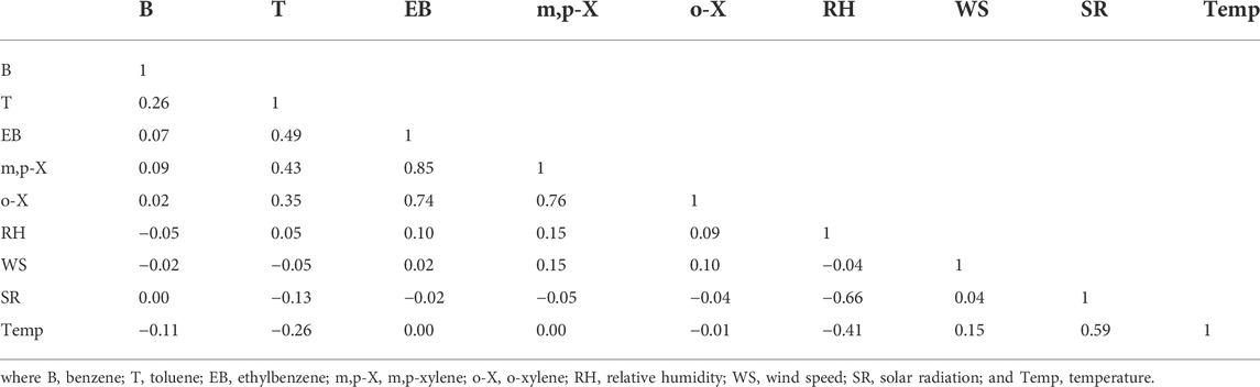
TABLE 3. Correlation matrix of BTEX concentrations with meteorological parameters.

We observe that the BTEX constituents have weak correlations with the local meteorological parameters, for example, the values range from −0.11 to 0.0 for B. A weak correlation of BTEX constituents with meteorological parameters indicates that BTEX variations are independent of climatic conditions at the sampling site. The results also suggest that the potential sources responsible for the emission of BTEX must be at a longer distance from the sampling site. On the other hand, as expected, the meteorological parameters are highly correlated with each other. Except for wind speed, the weather parameters are more or less dependent on each other. For example, solar radiation and temperature have a moderate positive correlation, whereas negative correlation has been observed between humidity and solar radiation.

4.4 Seasonal and diurnal variations of benzene, toluene, ethyl benzene, and xylene

Figure 3 shows the average seasonal distributions of BTEX over Bhubaneswar. It can be noted that the concentrations are relatively lower for the pre-monsoon (Figure 3A) and monsoon seasons (Figure 3B) compared to those of the post-monsoon (Figure 3C) and winter seasons (Figure 3D). Diurnal meteorology conditions such as planetary boundary layer (PBL) heights, wind speed, and temperature can also affect the diurnal variation of pollutants significantly. In the pre-monsoon season, higher PBL heights, high temperatures over the area (Sahu et al., 2020) also support the lower concentrations of BTEX over the site. The lower concentrations during pre-monsoon and monsoon can also be attributed to the rainfall occurrence in these two seasons due to thunderstorms and monsoons, respectively. The concentration ranges of B and T show a substantial variation, while EB, m,p-X, and o-X have lower ranges of concentrations. In the case of T, the highest concentrations were observed during the winter season, whereas the post-monsoon season recorded the maximum values of B, EB, m,p-X, and o-X concentrations. The results show that each constituent of BTEX has maximum/minimum values in different seasons, and does not have any specific seasonal pattern.

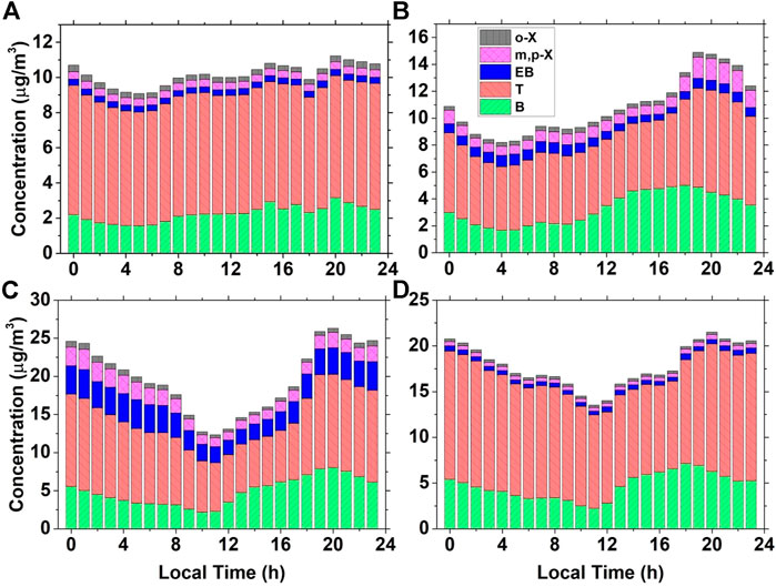
FIGURE 3. Wind rose plots at the sampling site in (A) pre-monsoon, (B) monsoon, (C) post-monsoon, and (D) winter.

The diurnal variability is least during the pre-monsoon season (Figure 3A). However, the higher ranges from late afternoon to night hours (1,500–2,300) are visible for other seasons (Figures 3B–D). The BTEX concentrations go to the lowest values during early morning hours, but the time for minimum value shifts from 5:00 h (pre-monsoon and monsoon) to 1,000 h (post-monsoon and winter), respectively. These minimum value ranges can be understood as the hours with no BTEX generation during the previous hours and the current hour of values. The results indicate that during the post-monsoon and winter seasons, the 1,000 h show the minimum concentration of BTEX; it is quite evident that emissions during office hours of the morning at the local scale do not impact the values. These variations indicate that the transported pollution may maintain the concentrations at the site from nearby regions. The average diurnal variations for BTEX show no particular pattern of the changes as well.

4.5 Tracing potential sources of transportation

Two-day-old trajectories (isentropic) have been computed using the HYSPLIT model, with GDAS (global data assimilation system) 1-degree data sets (Figure 4). We performed the cluster analysis based on Euclidean distance with the back trajectories, accounting for 2 days (−48 h) starting at the site. A total of 5,840 trajectories (6-h interval) have been obtained for the study over different seasons. The four different colors are chosen for different seasons, that is., red color indicates the trajectories in the pre-monsoon season, whereas blue, green, and black colors represent the trajectories during monsoon, post-monsoon, and winter season, respectively. The thin-colored lines represent the back trajectories, whereas the thick-colored lines depict the clusters for the total observation period. The yellow star represents the sampling site: Bhubaneswar.

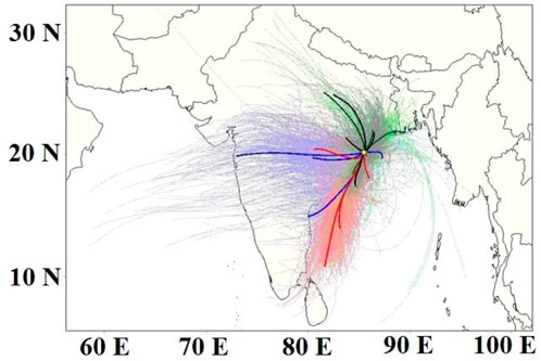
FIGURE 4. The back trajectory and cluster analysis at the sampling site (marked with a yellow star) during post-monsoon (green color), winter (black color), pre-monsoon (red color), and monsoon (blue color). Thin lines represent the back trajectories, while thick lines represent clusters for respective seasons.

It had been observed that during the post-monsoon and winter seasons, the transported air masses are generally approaching from the north, north-west, i.e., they are originated mostly from the Indo-Gangetic plains. The main regions of source for these air masses are Punjab, Uttar Pradesh, Bihar, and Delhi, which are pollution hotspots for BTEX concentrations (Srivastava et al., 2005b; Hoque et al., 2008; Sehgal et al., 2011; Chaudhary and Kumar, 2012; Singh et al., 2012; Bhattacharya and Tangri, 2015; Gaur et al., 2016; Singh et al., 2016; Kumar et al., 2017; Kumar et al., 2018; Masih et al., 2018; Garg et al., 2019). Interestingly, these air masses approach the site by crossing the metropolitan city of Kolkata followed by northern and central Odisha, which are few major pollution hotspots, and can be a probable source for the transported BTEX to the study site (Chattopadhyay et al., 1996; Dutta et al., 2009; Majumdar et al., 2011).

During the pre-monsoon season, the back trajectories mainly come from the Bay of Bengal. In contrast, during the monsoon season, the back trajectories show a wide range for the origination extending from the parts of central India to western India, as well as originating over the Arabian Sea. The transported air masses are mostly marine in the pre-monsoon and monsoon seasons, and the rainfall during these seasons also work as rainout and washout of pollutants, which may be the reason for the reduced BTEX concentrations at the site, which indicates that BTEX concentrations during these seasons are results of local emissions over the region.

4.6 Assessment of local transportation emissions

For the assessment of the local transportation sector and related emissions, we surveyed the total roads and vehicles for the year 2018. Table 4 depicts the major, minor, national, and state highway roads surveyed and the total vehicles on these roads. Higher traffic density was found in Hansapal Square, Palasuni, Baramunda (Kali Mandir), Dumduma Chowk, Kalpana Square, Ravi Talkies Chowk, Ouat Siripur, Kalinga Hospital Chowk, Chandrasekharpur (Tanishq), Damana Square, Patia Chowk, and Kiit Square. The Sikharchandi Chowk, Sailashree Vihar (Jagannath Temple), Buddha Park, Mancheswar Railway Stadium Road, Sparsh Hospital Road, Saheed Nagar (Jagannath Hos. Road), Saheed Nagar (Veterinary Hos.), Chandaka, Sainik School, and Pandra Square received the lowest traffic density. The emission patterns are in line with what the vehicles encountered on the road, and we have calculated the total emissions for CO and NOX for the year 2018.

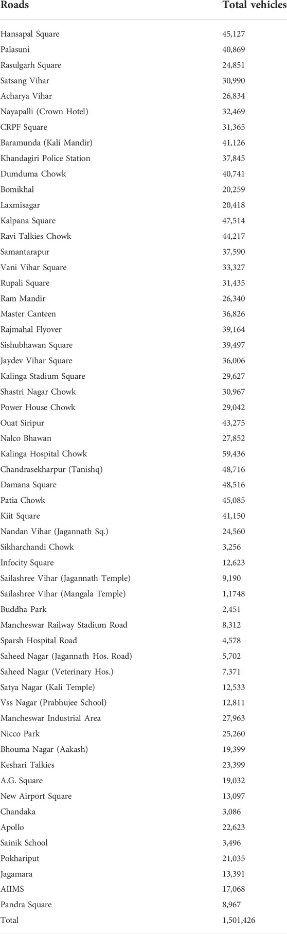
TABLE 4. Roads surveyed and total vehicles in Bhubaneswar (including major, minor, national, and state highways) for the year 2018.

Figures 5, 6 account for the total CO and NOX emissions over Bhubaneswar for the year 2018. It is clear from both the CO and NOX emissions that the city centre has higher emissions which are also consistent with higher traffic density encountered in the respective areas. The outskirts of Bhubaneswar are showing drastic reductions in both CO and NOx values. To further detail the total vehicles according to the type and fuel used, we have calculated the information about different vehicle types, their fuel used, and the total distance traveled by them per day (Table 5). The analysis revealed that the city had the highest numbers of two wheelers (908435), which runs on petrol with an average vehicle kilometer traveled (VKT/day) of 60. For diesel vehicles, three wheelers accounted for the highest share (211818) with a VKT/day of 150. As the BTEX concentrations are found to be higher in traffic emissions, with the spatial patterns of CO and NOx over the city, we can suggest the regions based on the information from Figures 5, 6 and Tables 3, 4 with possibly higher values of BTEX over the city.

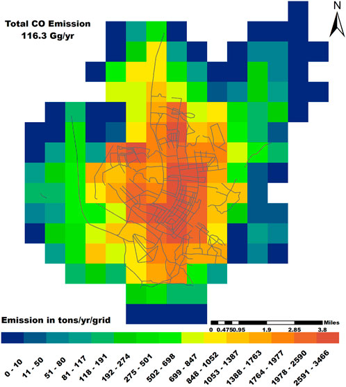
FIGURE 5. Total carbon monoxide emissions (Gg/year) over the smart city of Bhubaneswar for the year 2018 for 1 km × 1 km resolution, considering the transportation sector.

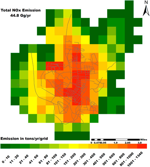
FIGURE 6. Total NOX emissions (Gg/year) over the smart city of Bhubaneswar for the year 2018 for 1 km × 1 km resolution considering the transportation sector.

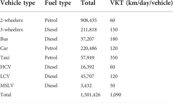
TABLE 5. Total number of vehicles on road and vehicles’ kilometer traveled (VKT/day) for Bhubaneswar city for the year 2018.

4.7 Emission inventory for nitrogen oxides, volatile organic compounds, and carbon monoxide over Bhubaneswar

A high-resolution emission inventory (EI) of the eight primary air pollutants has been developed for Bhubaneswar, one of the non-attainment cities of Odisha taking the base year as 2018. The emission of gaseous pollutants such as CO, NOx, SO₂, and VOC as well as particulate matter PM_2.5, PM₁₀, BC, and OC have been considered here from all possible major and minor sectors. Wind-blown road dust, transport, industry, residential cooking activities, and other minor sectors were incorporated in our study. The estimations for CO, NOx, SO₂, VOC, PM_2.5, PM₁₀, BC, and OC are found to be 111.58 Gg/yr, 44.41 Gg/yr, 10.58 Gg/yr, 72.84 Gg/yr, 8.89 Gg/yr, 16.51 Gg/yr, 4.61 Gg/yr, and 5.09 Gg/yr, respectively. It has been found that the transport sector is the dominant sector for all the gaseous pollutants. The sector specific emissions of NOx, VOC, and CO have been illustrated in Figures 7, 8, and 9, respectively. In case of the gaseous pollutant NOx, the total emission was found to be 44.41 Gg/yr. The major amount of NOx with an approx. emission of ∼36.2 Gg/yr that comes from traffic, which solely holds 82% of the total NOx emission over the city followed by the industrial and aviation sectors with an emission of ∼2 Gg/yr each. On the other hand, a negligible amount of VOC is emitted by the residential and other sectors as 99 % of VOC comes from vehicular activities with an emission of ∼72.5 Gg/yr. The pollutant with maximum emissions was found to be CO with an overall emission of ∼111.5 Gg/yr. As incomplete combustion of fuel is the reason behind the emission of CO, it has been dominantly emitted from the combustion of fossil fuel and bio-fuel in vehicular engines and residential cooking activities, respectively. The transport sector was found to be emitting ∼98.4 Gg/yr of CO, whereas the cooking activities in households, slums, street vendors, etc. together contributed approximately 10.3 Gg/yr of CO. Apart from this, industry and other minor sectors show a lesser amount of CO emissions that is 0.3 Gg/yr and 2.4 Gg/yr, respectively.

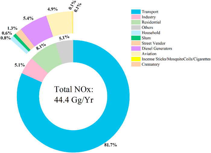
FIGURE 7. Contribution of NOX from major and minor sectors.

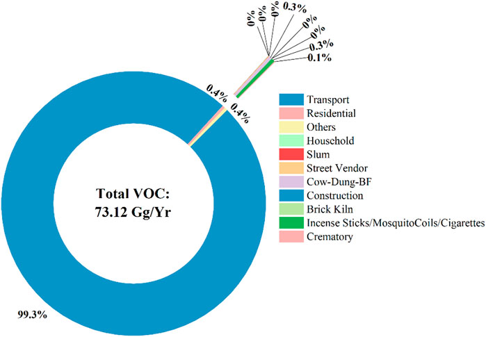
FIGURE 8. Contribution of VOC from major and minor sectors.

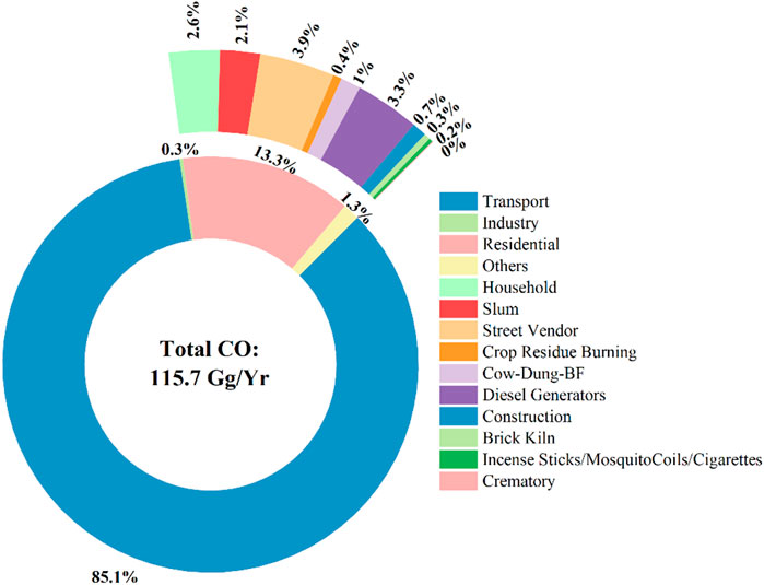
FIGURE 9. Contribution of CO from major and minor sectors.

5 Conclusion

The study analyzed the BTEX concentrations over Bhubaneswar, a tropical station along with various meteorological parameters and attempted to relate them with BTEX. The results can be summarized as follows:

• BTEX concentrations were independent of the local meteorological parameter variations.

• The BTEX during post-monsoon was comparatively higher than the winter months’ BTEX values. The BTEX concentrations in pre-monsoon and monsoon seasons were lower due to the wash-out effect in both locally generated and transported air. Moreover, the transport was oceanic at times during these two seasons, bringing clean air to the site.

• The BTEX concentrations were higher from the evening to late night during all seasons. However, the pre-monsoon season did not show variability in concentrations with time.

• The primary sources responsible for the emission of BTEX concentrations are a mix of both local and non-local. The primary suspected contributors may be vehicular emissions, local biomass-burning in hotels, and slum areas of Bhubaneswar, industrial locations in the northern parts of Central Odisha and Northern Odisha.

• The probable transported sources of BTEX concentrations came from the Indo-Gangetic plains of India, especially from states like Punjab, Uttar Pradesh, Bihar, and Delhi, which are pollution hotspots. The industrial zone over states like West Bengal, Odisha, and Jharkhand are also potential sources of BTEX to the study site.

• The city centre had higher CO and NOX emissions with higher traffic density and VKT/day for all types of vehicles and fuels. The study suggests that on a micro scale, the city centre has higher BTEX values associated with vehicular emissions compared to those of the outskirt areas.

• The highest contributions of NOX, VOC, and CO at Bhubaneswar came from the traffic. The contributions from residential and industrial sectors were existent, but not comparable to the vehicular emissions. The urban nature of the city further supported the findings, and the analysis shows that the hotspot regions of emissions are connected to the higher traffic density regions in the city.

The variability of NOX, VOC, and CO over the study region may also be modulated by the synoptic weather patterns (SWP) (Han et al., 2018). Zong et al. (2021) investigated the impact of SWP on ozone and PM_2.5 during the summer in eastern China. They classified the work’s SWPs from 500 hPa geopotential height (GPH) fields. Zong et al. (2022) analyzed 850 hPa GPH fields for categorizing the SWP and finding their influence on heatwaves and the ozone over Beijing, China. Previous studies also mostly utilized 850 hPa GPH fields for classifying SWP. The classification of SWP cannot be done by the surface GPH as the influence of surface conditions may incorporate inaccuracy in SWP classification (Han et al., 2018). The present study can benefit from the SWP classification; however, as the current results are based on surface observations, we are not proceeding with SWP classifications over our study region. Nevertheless, with the possible use of satellite data in future works, one should adopt the knowledge of SWPs over the area to find out the contributions of various SWPs.

Data availability statement

The data sets supporting the conclusion of this article will be made available by the authors, without undue reservation upon request.

Author contributions

SS: Collection of data, analysis of data, and writing—review and editing; BT: Analysis of data, writing the first draft of the manuscript, and writing—review and editing; RY: Analysis of data, writing the first draft of manuscript, and writing—review and editing; GB: Collection of data and writing—review, and editing; PM: Collection of data; OP: Analysis of data; SC: Analysis of data; ND: Review of manuscript; and PS: Review of manuscript.

Funding

Indian Institute of Tropical Meteorology (IITM), Ministry of Earth Science, Govt. of India, for funding the instrumented site under MAPAN program (grant no. MoES/Indo-Nor/PS-10/2015).

Acknowledgments

Authors want to thank the Indian Institute of Tropical Meteorology (IITM), Ministry of Earth Science, Govt. of India, for funding the instrumented site under the MAPAN program (grant no. MoES/Indo-Nor/PS-10/2015). We want to thank the HYSPLIT development team for providing the model and the National Center for Environmental Prediction (NCEP) for the GDAS data. Authors want to thank Utkal University and the National Institute of Technology, Rourkela, for providing research facilities for conducting this research.

Conflict of interest

The authors declare that the research was conducted in the absence of any commercial or financial relationships that could be construed as a potential conflict of interest.

Publisher’s note

All claims expressed in this article are solely those of the authors and do not necessarily represent those of their affiliated organizations, or those of the publisher, the editors, and the reviewers. Any product that may be evaluated in this article, or claim that may be made by its manufacturer, is not guaranteed or endorsed by the publisher.

References

Atkinson, R. (2000). Atmospheric chemistry of VOCs and NOX. Atmos. Environ. X. 34 (12-14), 2063–2101. doi:10.1016/s1352-2310(99)00460-4
Bauri, N., Bauri, P., Kumar, K., and Jain, V. K. (2016). Evaluation of seasonal variations in abundance of BTXE hydrocarbons and their ozone forming potential in ambient urban atmosphere of Dehradun (India). Air Qual. Atmos. Health 9 (1), 95–106. doi:10.1007/s11869-015-0313-z
Beig, G., Ghude, S. D., Polade, S. D., and Tyagi, B. (2008). Threshold exceedances and cumulative ozone exposure indices at tropical suburban site. Geophys. Res. Lett. 35 (2), L02802. doi:10.1029/2007gl031434
Bell, M. L., and Davis, D. L. (2001). Reassessment of the lethal london fog of 1952: Novel indicators of acute and chronic consequences of acute exposure to air pollution. Environ. Health Perspect. 109 (3), 389–394. doi:10.2307/3434786
Bhardwaj, V., Rani, B., and Kumar, A. (2017). Determination of BTEX in urban air of Agra. Int. J. Adv. Res. Sci. Eng. 6 (8), 801–808.
Bhattacharya, A., and Tangri, A. (2015). Monitoring of benzene, toluene, ethylbenzene and xylene (BTEX) concentration in ambient air in Kanpur, India2(9), Page: 1-4. Glob. J. Eng. Sci. Res. 2 (9), 1–4.
Bono, R., Scursatone, E., Schiliro, T., and Gilli, G. (2003). Ambient air levels and occupational exposure to benzene, toluene, and xylenes in northwestern Italy. J. Toxicol. Environ. Health A 66, 519–531. doi:10.1080/15287390306357
Chattopadhyay, G., Chatterjee, S., and Chakraborti, D. (1996). Determination of benzene, toluene and xylene in ambient air inside three major steel plant airsheds and surrounding residential areas. Environ. Technol. 17 (5), 477–488. doi:10.1080/09593331708616409
Chattopadhyay, G., Samanta, G., Chatterjee, S., and Chakraborti, D. (1997). Determination of benzene, toluene and xylene in ambient air of Calcutta for three years during winter. Environ. Technol. 18 (2), 211–218. doi:10.1080/09593331808616529
Chaudhary, S., and Kumar, A. (2012). Monitoring of benzene, toluene, ethylbenzene and xylene (BTEX) concentrations in ambient air in Firozabad, India. Int. Arch. Appl. Sci. Technol. 3 (2), 92–96.
Choudhury, G., Tyagi, B., Singh, J., Sarangi, C., and Tripathi, S. N. (2019). Aerosol-orography-precipitation–A critical assessment. Atmos. Environ. X. 214, 116831. doi:10.1016/j.atmosenv.2019.116831
da Silva, C. M., Corrêa, S. M., and Arbilla, G. (2020). Preliminary study of ambiente levels and exposure to BTEX in the rio de Janeiro olympic metropolitan region, Brazil. Bull. Environ. Contam. Toxicol. 104 (6), 786–791. doi:10.1007/s00128-020-02855-4
Derwent, R. G., Davies, T. J., Delaney, M., Dollard, G. J., Field, R. A., Dumitrean, P., et al. (2000). Analysis and interpretation of the continuous hourly monitoring data for 26 C2 – C6 hydrocarbons at 12 United Kingdom sites during 1996. Atmos. Environ. X. 34, 297–312. doi:10.1016/s1352-2310(99)00203-4
Dewangan, S., Chakrabarty, R., Zielinska, B., and Pervez, S. (2013). Emission of volatile organic compounds from religious and ritual activities in India. Environ. Monit. Assess. 185 (11), 9279–9286. doi:10.1007/s10661-013-3250-z
Draxler, R. R., and Hess, G. D. (1998). An overview of the HYSPLIT_4 modeling system for trajectories, dispersion, and deposition. Aust. Meteorol. Mag. 47, 295–308.
Dutta, C., Som, D., Chatterjee, A., Mukherjee, A. K., Jana, T. K., and Sen, S. (2009). Mixing ratios of carbonyls and BTEX in ambient air of Kolkata, India and their associated health risk. Environ. Monit. Assess. 148 (1-4), 97–107. doi:10.1007/s10661-007-0142-0
Garg, A., and Gupta, N. C. (2019). A comprehensive study on spatio-temporal distribution, health risk assessment and ozone formation potential of BTEX emissions in ambient air of Delhi, India. Sci. Total Environ. 659, 1090–1099. doi:10.1016/j.scitotenv.2018.12.426
Garg, A., Gupta, N. C., and Tyagi, S. K. (2019). Levels of benzene, toluene, ethylbenzene, and xylene near a traffic-congested area of East Delhi. Environ. Claims J. 31 (1), 5–15. doi:10.1080/10406026.2018.1525025
Garzón, J. P., Huertas, J. I., Magaña, M., Huertas, M. E., Cárdenas, B., Watanabe, T., et al. (2015). Volatile organic compounds in the atmosphere of Mexico City. Atmos. Environ. X. 119, 415–429. doi:10.1016/j.atmosenv.2015.08.014
Gaur, M., Singh, R., and Shukla, A. (2016). Variability in the levels of BTEX at a pollution hotspot in New Delhi, India. J. Environ. Prot. Irvine, Calif. 7 (10), 1245–1258. doi:10.4236/jep.2016.710110
Gogikar, P., and Tyagi, B. (2016). Assessment of particulate matter variation during 2011–2015 over a tropical station Agra, India. Atmos. Environ. X. 147, 11–21. doi:10.1016/j.atmosenv.2016.09.063
Gogikar, P., Tyagi, B., Padhan, R. R., and Mahaling, M. (2018). Particulate matter assessment using in situ observations from 2009 to 2014 over an industrial region of eastern India. Earth Syst. Environ. 2 (2), 305–322. doi:10.1007/s41748-018-0072-8
Golkhorshidi, F., Sorooshian, A., Jafari, A. J., Baghani, A. N., Kermani, M., Kalantary, R. R., et al. (2019). On the nature and health impacts of BTEX in a populated middle eastern city: Tehran, Iran. Atmos. Pollut. Res. 10 (3), 921–930. doi:10.1016/j.apr.2018.12.020
Hamid, H. H. A., Latif, M. T., Nadzir, M. S. M., Uning, R., Khan, M. F., and Kannan, N. (2019). Ambient BTEX levels over urban, suburban and rural areas in Malaysia. Air Qual. Atmos. Health 12 (3), 341–351. doi:10.1007/s11869-019-00664-1
Han, H., Liu, J., Yuan, H., Jiang, F., Zhu, Y., Wu, Y., et al. (2018). Impacts of synoptic weather patterns and their persistency on free tropospheric carbon monoxide concentrations and outflow in eastern China. J. Geophys. Res. Atmos. 123 (13), 7024–7046. doi:10.1029/2017jd028172
Helfand, W. H., Lazarus, J., and Theerman, P. (2001). Donora, Pennsylvania: An environmental disaster of the 20th century. Am. J. Public Health 91 (4), 1591. doi:10.2105/ajph.91.10.1591
Hinwood, A. L., Rodriguez, C., Runnion, T., Farrar, D., Murray, F., Horton, A., et al. (2007). Risk factors for increased BTEX exposure in four Australian cities. Chemosphere 66 (3), 533–541. doi:10.1016/j.chemosphere.2006.05.040
Hoque, R. R., Khillare, P. S., Agarwal, T., Shridhar, V., and Balachandran, S. (2008). Spatial and temporal variation of BTEX in the urban atmosphere of Delhi, India. Sci. Total Environ. 392 (1), 30–40. doi:10.1016/j.scitotenv.2007.08.036
Jemma, C. A., Shore, P. R., and Widdicombe, K. A. (1995). Analysis of C1-C16 hydrocarbons using dual-column capillary GC: Application to exhaust emissions from passenger car and motorcycle engines. J. Chromatogr. Sci. 33 (1), 34–48. doi:10.1093/chromsci/33.1.34
Karagulian, F., Belis, C. A., Dora, C. F. C., Prüss-Ustün, A. M., Bonjour, S., Adair-Rohani, H., et al. (2015). Contributions to cities' ambient particulate matter (PM): A systematic review of local source contributions at global level. Atmos. Environ. X. 120, 475–483. doi:10.1016/j.atmosenv.2015.08.087
Khoder, M. I. (2007). Ambient levels of volatile organic compounds in the atmosphere of Greater Cairo. Atmos. Environ. X. 41 (3), 554–566. doi:10.1016/j.atmosenv.2006.08.051
Kumar, A., Singh, D., Anandam, K., Kumar, K., and Jain, V. K. (2017). Dynamic interaction of trace gases (VOCs, ozone, and NOX) in the rural atmosphere of sub-tropical India. Air Qual. Atmos. Health 10, 885–896. doi:10.1007/s11869-017-0478-8
Kumar, A., Singh, D., Kumar, K., Singh, B. B., and Jain, V. K. (2018). Distribution of VOCs in urban and rural atmospheres of subtropical India: Temporal variation, source attribution, ratios, OFP and risk assessment. Sci. Total Environ. 613, 492–501. doi:10.1016/j.scitotenv.2017.09.096
Laowagul, W., and Yoshizumi, K. (2008). Characterization of benzene, toluene, ethylbenzene, and xylene concentrations in the ambient atmosphere of Tokyo, Japan. SEIKATSU EISEI J. Urban Living Health Assoc. 52 (5), 290–299.
Majumdar, D., Mukherjee, A. K., Mukhopadhaya, K., and Sen, S. (2012). Variability of BTEX in residential indoor air of Kolkata metropolitan city. Indoor Built Environ. 21 (3), 374–380. doi:10.1177/1420326x11409465
Majumdar, D., Mukherjee, A. K., and Sen, S. (2011). BTEX in ambient air of a Metropolitan City. J. Environ. Prot. Irvine, Calif. 2 (01), 11–20. doi:10.4236/jep.2011.21002
Majumdar, D., and Srivastava, A. (2012). Volatile organic compound emissions from municipal solid waste disposal sites: A case study of Mumbai, India. J. Air Waste Manag. Assoc. 62 (4), 398–407. doi:10.1080/10473289.2012.655405
Mangaraj, P., Sahu, S. K., Beig, G., and Samal, B. K. (2022a). Development and assessment of inventory of air pollutants that deteriorate the air quality in Indian megacity Bengaluru. J. Clean. Prod. 360, 132209. doi:10.1016/j.jclepro.2022.132209
Mangaraj, P., Sahu, S. K., Beig, G., and Yadav, R. (2022b). A comprehensive high-resolution gridded emission inventory of anthropogenic sources of air pollutants in Indian megacity Kolkata. SN Appl. Sci. 4, 117. doi:10.1007/s42452-022-05001-3
Masih, A., Lall, A. S., Taneja, A., and Singhvi, R. (2018). Exposure levels and health risk assessment of ambient BTX at urban and rural environments of a terai region of northern India. Environ. Pollut. 242, 1678–1683. doi:10.1016/j.envpol.2018.07.107
Miri, M., Shendi, M. R. A., Ghaffari, H. R., Aval, H. E., Ahmadi, E., Taban, E., et al. (2016). Investigation of outdoor BTEX: Concentration, variations, sources, spatial distribution, and risk assessment. Chemosphere 163, 601–609. doi:10.1016/j.chemosphere.2016.07.088
Mohan, S., and Ethirajan, R. (2012). Assessment of hazardous volatile organic compounds (VOC) in a residential area abutting a large petrochemical complex. J. Trop. For. Environ. 2 (1), 48–59. doi:10.31357/jtfe.v2i1.569
Monod, A., Sive, B. C., Avino, P., Chen, T., Blake, D. R., and Rowland, F. S. (2001). Monoaromatic compounds in ambient air of various cities: A focus on correlations between the xylenes and ethylbenzene. Atmos. Environ. X. 35 (1), 135–149. doi:10.1016/s1352-2310(00)00274-0
Nelson, P. F., and Quigley, S. M. (1983). The m, p-xylenes: Ethylbenzene ratio. A technique for estimating hydrocarbon age in ambient atmospheres. Atmos. Environ. 17 (3), 659–662.
Olson, K. L., Sinkevitch, R. M., and Sloane, T. M. (1992). Speciation and quantitation of hydrocarbons in gasoline engine exhaust. J. Chromatogr. Sci. 30 (12), 500–508. doi:10.1093/chromsci/30.12.500
Paatero, P., and Hopke, P. K. (2003). Discarding or downweighting high-noise variables in factor analytic models. Anal. Chim. Acta X. 490, 277–289. doi:10.1016/s0003-2670(02)01643-4
Rekhadevi, P. V., Rahman, M. F., Mahboob, M., and Grover, P. (2010). Genotoxicity in filling station attendants exposed to petroleum hydrocarbons. Ann. Occup. Hyg. 54 (8), 944–954. doi:10.1093/annhyg/meq065
Sahu, L. K., Pal, D., Yadav, R., and Munkhtur, J. (2016). Aromatic VOCs at major road junctions of a metropolis in India: Measurements using TD-GC-FID and PTR-TOF-MS instruments. Aerosol Air Qual. Res. 16, 2405–2420. doi:10.4209/aaqr.2015.11.0643
Sahu, L. K., and Saxena, P. (2015). High time and mass resolved PTR-TOF-MS measurements of VOCs at an urban site of India during winter: Role of anthropogenic, biomass burning, biogenic and photochemical sources. Atmos. Res. 164, 84–94. doi:10.1016/j.atmosres.2015.04.021
Sahu, R. K., Dadich, J., Tyagi, B., Vissa, N. K., and Singh, J. (2020). Evaluating the impact of climate change in threshold values of thermodynamic indices during pre-monsoon thunderstorm season over Eastern India. Nat. Hazards (Dordr). 102, 1541–1569. doi:10.1007/s11069-020-03978-x
Sahu, S. K., Tyagi, B., Pradhan, C., and Beig, G. (2019). Evaluating the variability, transport and periodicity of particulate matter over smart city Bhubaneswar, a tropical coastal station of eastern India. SN Appl. Sci. 1 (5), 383. doi:10.1007/s42452-019-0427-2
Sahu, S. K., Beig, G., and Parkhi, N. S. (2011). Emissions inventory of anthropogenic PM2. 5 and PM10 in Delhi during commonwealth games 2010. Atmos. Environ. X. 45 (34), 6180–6190. doi:10.1016/j.atmosenv.2011.08.014
Sahu, S. K., Tyagi, B., Beig, G., Mangaraj, P., Pradhan, C., Khuntia, S., et al. (2020b). Significant change in air quality parameters during the year 2020 over 1st smart city of India: Bhubaneswar. SN Appl. Sci. 2 (12), 1990–1998. doi:10.1007/s42452-020-03831-7
Sarkar, C., Chatterjee, A., Majumdar, D., Ghosh, S. K., Srivastava, A., and Raha, S. (2014). Volatile organic compounds over eastern himalaya, India: Temporal variation and source characterization using positive Matrix factorization. Atmos. Chem. Phys. Discuss. 14 (23), 32133–32175. doi:10.5194/acpd-14-32133-2014
Sehgal, M., Suresh, R., Sharma, V. P., and Gautam, S. K. (2011). Variations in air quality at filling stations, Delhi, India. Int. J. Environ. Stud. 68 (6), 845–849. doi:10.1080/00207233.2012.620320
Singh, A. K., Tomer, N., and Jain, C. L. (2012). Monitoring, assessment and status of benzene, toluene and xylene pollution in the urban atmosphere of Delhi, India. Res. J. Chem. Sci. 2 (4), 45–49. doi:10.1100/2012/272853
Singh, D., Kumar, A., Singh, B. P., Anandam, K., Singh, M., Mina, U., et al. (2016). Spatial and temporal variability of VOCs and its source estimation during rush/non-rush hours in ambient air of Delhi, India. Air Qual. Atmos. Health 9 (5), 483–493. doi:10.1007/s11869-015-0354-3
Singh, R., Shukla, A., Gangopadhyay, S., and Adhikary, S. (2010). A pilot study of benzene in different corridors of Delhi. Indian J. Air Pollut. Control X (1), 21–24.
Singla, V., Pachauri, T., Satsangi, A., Kumari, K. M., and Lakhani, A. (2012). Comparison of BTX profiles and their mutagenicity assessment at two sites of Agra, India. Sci. World J 2012, 272853. doi:10.1100/2012/272853
Smart Cities Mission (2017). Smart cities mission. Avaliable At: http://smartcities.gov.in/content/.
Som, D., Dutta, C., Chatterjee, A., Mallick, D., Jana, T. K., and Sen, S. (2007). Studies on commuters' exposure to BTEX in passenger cars in Kolkata, India. Sci. Total Environ. 372 (2-3), 426–432. doi:10.1016/j.scitotenv.2006.09.025
Srivastava, A., Joseph, A. E., and Devotta, S. (2006). Volatile organic compounds in ambient air of Mumbai—India. Atmos. Environ. X. 40 (5), 892–903. doi:10.1016/j.atmosenv.2005.10.045
Srivastava, A., Joseph, A. E., More, A., and Patil, S. (2005a). Emissions of VOCs at urban petrol retail distribution centres in India (Delhi and Mumbai). Environ. Monit. Assess. 109 (1-3), 227–242. doi:10.1007/s10661-005-6292-z
Srivastava, A., Sengupta, B., and Dutta, S. A. (2005b). Source apportionment of ambient VOCs in Delhi City. Sci. Total Environ. 343 (1-3), 207–220. doi:10.1016/j.scitotenv.2004.10.008
Tyagi, B., Singh, J., and Beig, G. (2020). Seasonal progression of surface ozone and NOx concentrations over three tropical stations in North-East India. Environ. Pollut. 258, 113662. doi:10.1016/j.envpol.2019.113662
Yadav, R., Sahu, L. K., Beig, G., and Jaaffrey, S. N. A. (2016). Role of long-range transport and local meteorology in seasonal variation of surface ozone and its precursors at an urban site in India. Atmos. Res. 176, 96–107. doi:10.1016/j.atmosres.2016.02.018
Yadav, R., Beig, G., Anand, V., Kalbande, R., and Maji, S. (2022). Tracer-based characterization of source variations of ambient isoprene mixing ratios in a hillocky megacity, India, influenced by the local meteorology. Environ. Res. 205, 112465. doi:10.1016/j.envres.2021.112465
Zalel, A., and Broday, D. M. (2008). Revealing source signatures in ambient BTEX concentrations. Environ. Pollut. 156 (2), 553–562. doi:10.1016/j.envpol.2008.01.016
Zhang, Y., Mu, Y., Liu, J., and Mellouki, A. (2012). Levels, sources and health risks of carbonyls and BTEX in the ambient air of Beijing, China. J. Environ. Sci. 24 (1), 124–130. doi:10.1016/s1001-0742(11)60735-3
Zong, L., Yang, Y., Gao, M., Wang, H., Wang, P., Zhang, H., et al. (2021). Large-scale synoptic drivers of co-occurring summertime ozone and PM<sub>2.5</sub> pollution in eastern China. Atmos. Chem. Phys. 21 (11), 9105–9124. doi:10.5194/acp-21-9105-2021
Zong, L., Yang, Y., Xia, H., Gao, M., Sun, Z., Zheng, Z., et al. (2022). Joint occurrence of heatwaves and ozone pollution and increased health risks in beijing, China: Roles of synoptic weather pattern and urbanization. Atmos. Chem. Phys. Discuss. 22, 1–29. doi:10.5194/acp-22-6523-2022
Keywords: BTEX, VOCs, seasonal variation, smart city, air quality
Citation: Sahu SK, Mangaraj P, Tyagi B, Yadav R, Paul O, Chaulya S, Pradhan C, Das N, Sahoo P and Beig G (2022) Estimating NOX, VOC, and CO variability over India’s 1st smart city: Bhubaneswar. Front. Environ. Sci. 10:997026. doi: 10.3389/fenvs.2022.997026
Received: 18 July 2022; Accepted: 29 August 2022;
Published: 28 September 2022.
Edited by:
Zengyun Hu, Chinese Academy of Sciences (CAS), ChinaReviewed by:
Yuanjian Yang, Nanjing University of Information Science and Technology, ChinaJiawei Li, Institute of Atmospheric Physics (CAS), China
Copyright © 2022 Sahu, Mangaraj, Tyagi, Yadav, Paul, Chaulya, Pradhan, Das, Sahoo and Beig. This is an open-access article distributed under the terms of the Creative Commons Attribution License (CC BY). The use, distribution or reproduction in other forums is permitted, provided the original author(s) and the copyright owner(s) are credited and that the original publication in this journal is cited, in accordance with accepted academic practice. No use, distribution or reproduction is permitted which does not comply with these terms.
*Correspondence: Bhishma Tyagi, tyagib@nitrkl.ac.in