A Demand-Side Load Event Detection Algorithm Based on Wide-Deep Neural Networks and Randomized Sparse Backpropagation

Introduction

Event detection is a crucial technique in power systems to avoid emergencies, such as blackouts and equipment impairments, through fault and disturbance detection (Ma et al., 2019). Due to the importance of maintaining the stability and reliability of the power system, traditional research focuses on system-side event detection which perceives extreme events using the high-frequency phasor measurement unit (PMU) data (Biswal et al., 2016; Liu et al., 2019; Ma et al., 2020). As smart meters become more accessible, many researchers focus on demand-side event detection that monitors smart home activities using low-frequency data. Smart home activities occur when homeowners switch on or off their appliances. These two events are significant because they contain plenty of behavioral information about the homeowners. This information helps users understand their electricity usage behaviors and reduce energy costs.

Existing research in event detection can be divided into four categories: rule-based, statistic-based, conventional machine learning, and deep learning. For rule-based methods, (Shaw and Jena, 2020), observes an event if the standard deviation (std.) of the phase angle difference or the rate of change of frequency (ROCOF) exceeds a given threshold. In (Pandey et al., 2020), a physic-based rule is applied to classify active power, reactive power, and fault events according to the cluster change. For statistic-based methods, (Pandey et al., 2020), also designs base event detectors using linear regression and Chebyshev inequality, both of which require manually specified thresholds. Subsequently, synchrophasor anomaly detection is carried out by maximum likelihood estimation. For conventional machine learning methods, the K-Nearest Neighbor (KNN) approach is used for the feature selection task that discovers typical characteristics of disturbance types (Biswal et al., 2016). In (Mishra et al., 2015), the decision tree algorithm is used for fault detection and classification in microgrid protection based on 15 independent wavelet coefficients. For deep-learning algorithms, (Wang et al., 2020), indicates that GPU-based deep learning has been applied to solve various problems in power systems including event classification, NILM, and load forecasting. In their work, ROCOF and relative angle shift are converted into images before being analyzed by two CNNs. In (James et al., 2017), a deep neural network based on Gated Recurrent Units and Discrete Wavelet Transform is used for solving the microgrid fault detection problem. Li et al. (2021) proposes a deep learning framework for load recognition based on a deep-shallow model and a fast backpropagation algorithm.

The rule-based approach for event detection has lower model complexity and requires less computation time (Shaw and Jena, 2020). However, it has three main disadvantages. First, tremendous efforts are required for manual feature engineering. Second, thresholds need to be carefully calibrated based on human expertise. Third, rule-based models may not adapt well to the new data. As for statistics-based or conventional machine learning methods, although the training time is short and the interpretability is good, the accuracy is inferior to deep learning models caused by the complex feature under-fitting. The performance of deep learning algorithms has significantly surpassed the competitors from the conventional machine learning field and other hand-crafted AI systems (Goodfellow et al., 2016) partly because of their excellent automatic feature extraction capability. However, training a deep learning model is time-consuming and requires an intensive amount of computational resources. Also, the inherent complexity of deep models makes them elusive to interpret.

Therefore, by combining statistics-based methods, conventional machine learning approaches, and deep learning algorithms, a model can be created that is fast to train, easy to interpret, and most importantly, possesses great generalization ability. The Wide and Deep Learning (Cheng et al., 2016) proposed by Google offers a solution to this task in that both memorization and generalization are attenable by jointly training a linear model and a deep neural network. The DeepFM model (Guo et al., 2017) is proposed for recommendation systems in which the deep model is used for feature learning and recommendation is accomplished by the wide factorization machine model.

This paper focuses on load event detection in smart homes. A load event is defined as a sudden change of load caused by the activities of users. The switch-on and switch-off events are two common load events that happen in residential buildings. To detect a load event, a wide-deep model is created based on the idea of Wide and Deep Learning to jointly train a deep CNN and a wide SMR for detecting the occurrence of an appliance switch-on or switch-off event. The deep model uses the normalized active and apparent power time series as inputs. The wide model uses outputs from the deep model and the percentile information of the power time series as inputs. To prevent the model quality degradation problem in CNN caused by the noisy, incomplete, and low-quality training data, the randomized sparse backpropagation (RSB) algorithm for weight filters is proposed to improve the robustness of the standard wide-deep model. The pure CNN model, pure SMR model, and KNN algorithm are compared with the standard wide-deep model. And a hybrid wide-deep model with RSB applied to the last convolution layer of the deep model is compared with the standard wide-deep model.

This Paper Makes the Following Contributions

1) The standard wide-deep model is proposed that combines CNN and SMR to detect smart home appliance switch-on and switch-off events. The proposed model has a faster convergence speed and a higher accuracy compared to pure CNN and SMR.

2) Percentile information of active and apparent power time series is utilized by SMR to facilitate training and improve interpretability.

3) The randomized sparse backpropagation algorithm for weight filters is proposed to improve the robustness of the standard wide-deep model and accelerate training by reducing the number of multiplications.

This paper is organized as follows: Section 2 introduces the proposed wide-deep model that combines CNN and SMR; Section 3 describes the RSB algorithm in detail; Section 4 describes how training data is collected and compares the performance of the wide-deep model (hybrid and standard), pure CNN, pure SMR, and KNN. Section 5 summarizes the entire paper.

Wide-Deep Model

A wide-deep model that combines the statistics-based method, conventional machine learning, and deep learning is proposed for load event detection in smart homes, inspired by Wide and Deep Learning (Cheng et al., 2016). The deep model is a CNN that analyzes complex features of the active and apparent power time series. The wide model is an SMR that accepts CNN outputs and the percentile information of the power time series as inputs before event detection. There are two kinds of detectable events in this work: switch-on and switch-off events. Other than that, the model outputs a null event.

Deep Model

Local connection, shared weights, pooling, and usage of multiple layers are four remarkable characteristics of CNN (LeCun et al., 2015). CNN is suitable for event detection tasks for three reasons: First, local power time series data are highly correlated. Second, the location invariance of load, e.g. switch-on events in a time window show similar characteristics no matter when they happen, makes it appropriate to use shared weights. Third, composing lower-level features of the power time series to obtain higher-level features greatly improves the model’s analytical abilities.

Although recurrent neural networks (RNN) (Schuster and Paliwal, 1997) are also suited for sequence processing, vanishing and exploding gradients problems should be effectively addressed (Hochreiter and Schmidhuber, 1997). Unlike hardware-accelerated CNN that takes full advantage of graphical processing units (GPU), RNN requires a much longer training time due to the necessity to create a long chain of RNN cells. Stand-alone artificial neural networks (ANN) ignore the correlation information in the time domain which is crucial for time series data processing (James et al., 2017). When the dataset is large and the dimension is high, KNN becomes time-consuming because of the requirement for a myriad of distance calculations. Above all, CNN is chosen by the deep model for event detection. This is contrary to the original wide and deep learning (Cheng et al., 2016) in which the deep model is a pure ANN.

To fully exploit the automatic feature extraction ability of CNN, input data should be properly pre-processed. For each training sample, the input is a $2\times (T+1)$ matrix, where $T$ is the length of the time window. In this paper, a 30-s time window is used which makes $T=30$. The first and second rows of the matrix store the normalized active and apparent power time series. The raw power time series are normalized in two steps: Firstly, define either the active or apparent power time series as a vector $\mathbf{p}$, the series is normalized using the following min-max approach:

Secondly, ${\mathbf{p}}_m$ is further normalized by its mean and standard deviation:

Besides, the deep model focuses more on the relationships among or the relative positions of the locally connected scalars in the power time series rather than their actual magnitude, which makes input normalization suitable for this scenario.

Although the shapes of active and apparent power time series are highly correlated, using both for CNN training augments the data set and may alleviate the over-fitting problem because power factor difference among various appliances increases data diversity. When training data are limited, CNN can be easily down-scaled to a simpler one that only uses either the active or apparent power time series as the inputs.

The CNN in this paper consists of three convolution layers and one fully connected (FC) layer. The first convolution layer has 24 filters, each filter has a height of 1 and a width of 9. The second convolution layer has 48 filters, each filter has a height of 1 and a width of 7. The third convolution layer has 96 filters, each filter has a height of 1 and a width of 5. The FC layer accepts outputs from the third convolution layer and has an output feature dimension of 60. The row and column strides for all filters are 1. Normalization and leaky-relu activation function with a slope of 0.01 on the negative side are applied to all convolution and FC layers. Max-pooling is not used by the convolution layers because it shrinks the length of the power time series and causes information loss. Figure 1 shows the architecture of the deep model.

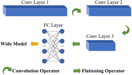
FIGURE 1. Architecture of the deep model. Notes: Conv denotes convolution; The blue cubic bars represent feature map tensors of CNN.

Wide Model

The CNN-based deep model automatically extracts and analyzes complex features from input data and shows great generalization ability when given unforeseen data. However, CNN has drawbacks in several aspects: First, training large CNN models is time-consuming. Second, plenty of high-quality statistics, e.g. mean, std., percentiles, etc., are submerged in the input data, which makes CNN harder to converge. Third, deep models are always difficult to interpret.

Therefore, a wide model based on SMR is designed to compensate for the downsides of the deep model. The wide model accepts outputs from the final FC layer of CNN, collects percentile information of the active and apparent power time series, and combines two parts of the data before training the SMR for event detection using the cross-entropy loss (Goodfellow et al., 2016).

The power time series percentile information is collected as follows. Let $\mathbf{p}=(p_1,p_2,\dots ,p_{T+1})$ be the active or apparent power time series vector. Perform the one-step differentiation to extract features of abrupt changes:

If $\mathbf{p}$ is stable, the mean of $\Delta \mathbf{p}$ is zero. When a switch-on event occurs, there will be a positive scalar in $\Delta \mathbf{p}$ which is significantly larger than the rest due to the overall load increase. Likewise, when a switch-off event happens, there will be a negative scalar in $\Delta \mathbf{p}$ which is significantly lower than the rest because of the overall load drops. If $\mathbf{p}$ is unstable, half of the scalars in $\Delta \mathbf{p}$ may be positive while the rest are negative. Since the wide model is not designed to process a large amount of data like the deep model, only a part of scalars are chosen from $\Delta \mathbf{p}$ as the inputs. To extract representative features, the 0^th, 25^th, 50^th, 75^th, and 100^th percentiles of $\Delta \mathbf{p}$ are selected to form a vector $\mathbf{\rho }$:

Where ${\rho }_{\theta }$ is the ${\theta }^{th}$ percentile of $\Delta \mathbf{p}$. To prevent precision overflow, $\mathbf{\rho }$ is normalized using the min-max approach:

Figure 2–4 offer diagrams of normalized percentiles for active and apparent power time series considering switch-on, switch-off, and null events. It can be observed that for the switch-on event, the normalized 100^th percentile is close to 1; for the switch-off event, the normalized 0^th percentile is close to -1; for the null event, the normalized 0^th percentile and 100^th percentile tend to be -1 and 1 respectively. These features are easily understood by SMR which speeds up the model convergence.

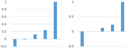
FIGURE 2. Normalized active and apparent power percentiles for a typical switch-on event.

FIGURE 3. Normalized active and apparent power percentiles for a typical switch-off event.

FIGURE 4. Normalized active and apparent power percentiles for a typical null event.

Figure 5 shows the architecture of the wide model, where ${\mathbf{\rho }}_m^{active}$ and ${\mathbf{\rho }}_m^{apparent}$ are ${\mathbf{\rho }}_m$ calculated using the active and apparent power time series. Notes that the wide model degenerates into a pure SRM if CNN outputs are not used.

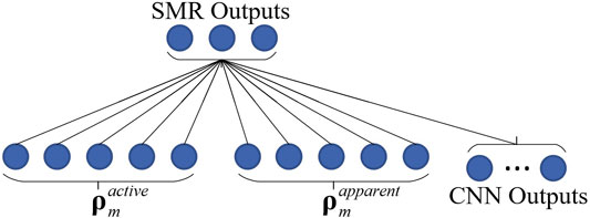
FIGURE 5. Architecture of the wide model.

The training example of the wide model is a 3-dimension one-hot vector, where ${\left(\mathrm{1,0,0}\right)}^T$ represents a null event, ${\left(\mathrm{0,1,0}\right)}^T$ represents a switch-on event, and ${\left(\mathrm{0,0,1}\right)}^T$ represents a switch-off event. Since the cross-entropy loss is utilized, each scalar in the SMR outputs describes the probability of each event.

Randomized Sparse Backpropagation

Noisy, incomplete, or low-quality training data for event detection hampers the CNN model quality. Inspired by the drop-out regularization (Srivastava et al., 2014) that prevents over co-adaptation by randomly disabling units and connections, this work improves the robustness of the standard wide-deep model, e.g. evading bad local minima and alleviating over-fitting problems, by balancing exploitation and exploration search. To speed up training, the number of multiplications can be reduced by creating sparsity in the feature map gradient tensors. This paper proposes a randomized sparse backpropagation algorithm that adds exploration search to the optimization process and speeds up gradient calculations.

Symbol Definition

Define $N$ as the number of training data points; $h$ as the training data point index, $h\in [1,N]$; $L_h$ as the loss function for the $h^{th}$ training data point; $R$ as the number of filters; $r$ as the filter index, $r\in [1,R]$; ${\mathbf{W}}_r$ as the $r^{th}$ 3-D filter tensor; $w$ as a scalar of ${\mathbf{W}}_r$ for a certain input channel, $w\in {\mathbf{W}}_r$; $u,v$ as the row and column indexes of $w$; $rs,cs$ as the filter row and column strides; $\partial L_h/\partial {\mathbf{W}}_r$ as the 3-D filter gradient tensor; ${\mathbf{X}}_h$ as the $h^{th}$ 3-D input tensor; $x$ as a scalar of ${\mathbf{X}}_h$ in a certain input channel, $x\in {\mathbf{X}}_h$; ${\mathbf{Z}}_h$ as the $h^{th}$ 3-D feature map tensor; ${\mathbf{Z}}_{h,r}$ as the $r^{th}$ output channel of ${\mathbf{Z}}_h$; $P,Q$ as the height and width of ${\mathbf{Z}}_h$; $z$ as a scalar of ${\mathbf{Z}}_h$ in the $r^{th}$ output channel, $z\in {\mathbf{Z}}_h$; $\partial L_h/\partial {\mathbf{Z}}_h$ as the 3-D feature map gradient tensor.

Randomized Sparse Backpropagation for Weight Filters

$\forall w^{\prime }\in \partial L_h/\partial {\mathbf{W}}_r$, $\exists \eta \ge 0$, such that the derivative of the loss function $L_h$ with respect to (w.r.t.) the filter scalar $w$ is defined as:

If $\left|{z^{\prime }}_{ij}\right|\ge \eta$, the indicator function $I=1$, otherwise $I=0$. Notice that every $w$ in ${\mathbf{W}}_r$ is independently assigned a random threshold $\eta$ that creates sparsity in $\partial L_h/\partial {\mathbf{Z}}_{h,r},h\in \left[1,N\right]$. Figure 6 illustrates the randomized sparse backpropagation process.

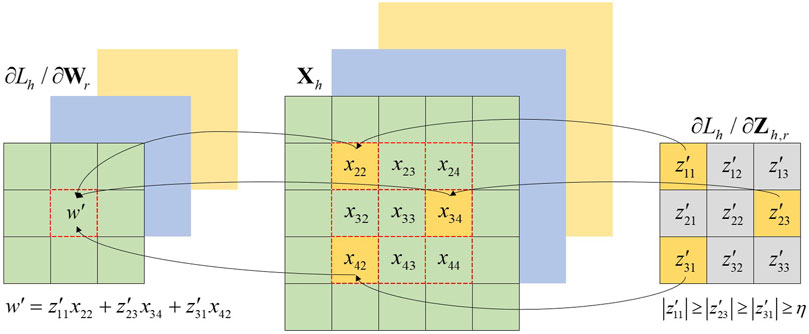
FIGURE 6. An example of the randomized sparse backpropagation for a filter. $P=3$, $Q=3$, $u=2$, $v=2$, $rs=1$, $cs=1N=1$.

The degree to which exploration search is conducted varies according to the random threshold $\eta$. When $\eta =0$, the algorithm becomes the standard backpropagation and involves no exploration search. As $\eta$ increases, the amount of the exploration search increases because ${z^{\prime }}_{ij}$ that has a smaller magnitude is not involved in the gradient calculations. When $\eta$ becomes excessively large, $w^{\prime }=0$ and $w$ is not changed. Therefore, every filter scalar $w$ may be fully, partially, or not updated. Besides, gradient calculations are accelerated due to the sparsity in the feature map gradient tensors. As $\eta$ increases from zero, the number of multiplications in calculating $w^{\prime }$ decreases because the condition $\left|{z^{\prime }}_{ij}\right|\ge \eta$ is less likely to be satisfied.

Determination of random threshold

The random threshold $\eta$ for the filter scalar $w$ is determined by the percentile approach without using any hyperparameters. Since $w$ is involved in the calculation of $N$ feature map matrixes ${\mathbf{Z}}_{h,r},h\in [1,N]$ in the forward pass, $w^{\prime }$ is related to $N$ feature map gradient matrixes $\partial L_h/\partial {\mathbf{Z}}_{h,r},h\in [1,N]$. These matrixes are firstly stacked into a 3-D tensor and then flattened to a vector. Subsequently, the abs function is applied to the vector, and scalars in the vector are sorted in ascending order. $\eta$ is defined as the ${\alpha }^{th}$ scalar of the sorted vector, where $\alpha$ is a uniform random integer between $1$ and $N\times P\times Q$. Figure 7 shows how $\eta$ is determined for $w$.

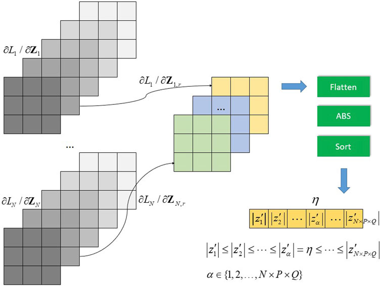
FIGURE 7. Determination of the random threshold $\eta$ for $w$.

Comparison to Related Works

The proposed RSB is inspired by (Wei et al., 2017) in which the top $k$ scalars in the feature map gradient tensors are used for updating the filter tensors. However, the value of $k$ has to be manually defined, and each $w$ does not have an independent $\eta$ for weight update. In (Ye et al., 2020), the pruning threshold is determined by two hyperparameters: the pruning rate and the std. of the feature map gradient tensors. (Wang and Nelaturu, 2019). offers a scaling approach to approximate the filter gradient tensors.

In RSB, no manual intervention is required because no hyperparameter is used. The exploration search that boosts the robustness of the standard wide-deep model is fulfilled in three aspects: First, each weight scalar $w$ is assigned an independent random threshold $\eta$. Second, $\eta$ is generated as a random variable using the percentile approach. Third, the filter gradient tensors are not precisely calculated on purpose.

Experiment

Training Data Collection

The UK-DALE dataset (Kelly and Knottenbelt, 2015) is used for all the experiments. Aggregated and appliance-level data are utilized in UK-DALE from houses 1, 2, and 5. The aggregated data has a sampling frequency of 1Hz and the appliance-level data has a sampling frequency of 6Hz. Both types of data include time series for active power, apparent power, and root mean square (RMS) voltages. Due to the low sampling frequency rate, the RMS voltage data are discarded and only the active and apparent power time series are used for training.

Since the UK-DALE dataset comes with a limited number of appliance on-off labels. The event dataset is derived from aggregated data with the help of the appliance-level data. Let (7) be the apparent power time series kernel vector extracted from the appliance-level data, where $n$ is an even number.

For a switch-on event, $s_i=0,s_j\ge \beta$; for a switch-off event, $s_i\ge \beta ,s_j=0$, where $\beta$ is a pre-defined threshold and $i\le n/2,j>n/2$. After several trials, $\beta =8\text{W}$, $n=10s$ are chosen for the data collection and cleaning procedures. When a switch-on or switch-off event is observed, the event timestamp is obtained from the appliance-level data. Then the active and apparent power time series with time window length $T=30s$ are acquired by querying the aggregated-level data using this timestamp. Since the null events data are abundant, the event dataset is established which includes 7,822 switch-on, 6,375 switch-off, and 7,102 null events. 90% of the data are used for training and 10% of the data are used for testing.

Model Training

All hybrid wide-deep, standard wide-deep, pure CNN, and pure SMR models are trained for 50 epochs and then compared. In the hybrid wide-deep model, RSB is only applied to its last convolution layer since the number of filter scalars in the last layer greatly exceeds the ones in the previous two layers. The pure SMR only accepts power time series percentile information as inputs, while the pure CNN does not utilize the percentile information. The experiments are conducted on a workstation with an Intel i7-9750H CPU, 16 GB of RAM, and an NVIDIA RTX 2060 GPU. All the algorithms are implemented using Java 11, C++ 17, and CUDA 10.2. The performance is evaluated by the convergence speed, training error, and test set accuracy. Figure 8–11 offer training error and test set accuracy diagrams for the hybrid wide-deep, standard wide-deep, pure CNN, and pure SMR models. Table 1 shows the epochs required and training errors when the maximum accuracies are firstly attained. The accuracy of KNN is also provided for comparison.

FIGURE 8. Training error and accuracy for the hybrid wide-deep model using the randomized sparse backpropagation.

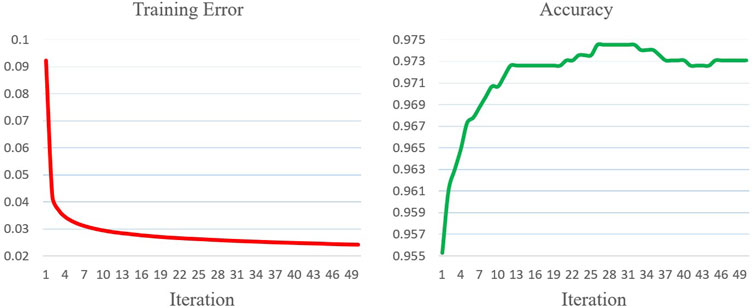
FIGURE 9. Training error and accuracy for the standard wide-deep model.

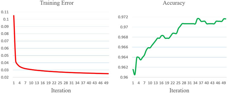
FIGURE 10. Training error and accuracy for the deep model.

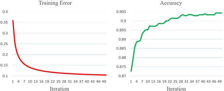
FIGURE 11. Training error and accuracy for the wide model.

TABLE 1. Model comparison.

The experiments show that the hybrid wide-deep model attains the best overall performance with the highest accuracy, fastest convergence speed, and minimal training error. Compared to the standard wide-deep model, the hybrid wide-deep model required 15% fewer epochs to obtain the max accuracy. Moreover, the accuracy curve is more stable than the one in the standard wide-deep model. This suggests that the exploration search incited by RSB speeds up convergence and improves the robustness of the standard wide-deep model. Compared to the pure CNN, the hybrid wide-deep model requires 37% fewer epochs to obtain the max accuracy, which demonstrates that the wide-deep model indeed speeds up neural network training and improves the accuracy by utilizing the power time series percentile information. Compared to the pure SMR, the hybrid wide-deep model requires 53% fewer epochs to obtain the max accuracy which is over 7% higher than the one for pure SMR. The pure SMR suffers from an under-fitting problem that the training error is always above 0.1 and the accuracy is inferior to KNN.

Conclusion

This paper proposes a wide-deep model for demand-side load event detection. The deep model is a CNN that extracts complex power time series features and the wide model is an SMR that analyzes percentile information of the power time series. The RSB algorithm for weight filters is proposed and applied to the last convolution layer of the deep model to improve the robustness of the standard wide-deep model. The hybrid wide-deep model has the highest test set accuracy, fastest convergence speed, and great robustness. Compared to the other models, the standard wide-deep model has the same accuracy as the hybrid one with a slightly slower convergence speed and more fluctuations in the accuracy curve. The pure CNN has a satisfactory accuracy but takes longer to converge. The pure SMR suffers from the under-fitting problem due to model simplicity. KNN has a medium accuracy but its classification time is long. In future research, more high-frequency data can be collected from smart homes to enable multi-task training, such as appliance classification, for the wide-deep model that helps homeowners better understand their electricity usage behaviors. RNN related algorithms can be combined with the wide-deep model to analyze more complex features. To render more accurate load event detection results, a multimodal deep learning framework can be created that combines the wide-deep model with smart home video processing systems (Li et al., 2019).

Data Availability Statement

The original contributions presented in the study are included in the article. Further inquiries can be directed to the corresponding author.

Author Contributions

CL: Conceptualization, Programming, Draft Writing; GL: Methodology, Revision; HZ: Reviewing, Revision; GC: Revision.

Conflict of Interest

The authors declare that the research was conducted in the absence of any commercial or financial relationships that could be construed as a potential conflict of interest.

The reviewer WK declared a shared affiliation with one of the authors, CL, to the handling editor at time of review

Publisher’s Note

All claims expressed in this article are solely those of the authors and do not necessarily represent those of their affiliated organizations, or those of the publisher, the editors and the reviewers. Any product that may be evaluated in this article, or claim that may be made by its manufacturer, is not guaranteed or endorsed by the publisher.

References

Biswal, M., Brahma, S. M., and Cao, H. (2016). Supervisory protection and Automated Event Diagnosis Using PMU Data. IEEE Trans. Power Deliv. 31 (4), 1855–1863. doi:10.1109/tpwrd.2016.2520958
Cheng, H. T., Koc, L., Harmsen, J., Shaked, T., Chandra, T., Aradhye, H., et al. (2016). “Wide & Deep Learning for Recommender Systems,” in Proceedings of the 1st Workshop on Deep Learning for Recommender Systems, 7–10. doi:10.1145/2988450.2988454
Goodfellow, I., Bengio, Y., Courville, A., and Bengio, Y. (2016). Deep Learning, Vol. 1. Cambridge: MIT press–2.
Guo, H., Tang, R., Ye, Y., Li, Z., and He, X. (2017). DeepFM: A Factorization-Machine Based Neural Network for CTR Prediction.
Hochreiter, S., and Schmidhuber, J. (1997). Long Short-Term Memory. Neural Comput. 9 (8), 1735–1780. doi:10.1162/neco.1997.9.8.1735
James, J. Q., Hou, Y., Lam, A. Y., and Li, V. O. (2017). Intelligent Fault Detection Scheme for Microgrids with Wavelet-Based Deep Neural Networks. IEEE Trans. Smart Grid 10 (2), 1694–1703.
Kelly, J., and Knottenbelt, W. (2015). The UK-DALE Dataset, Domestic Appliance-Level Electricity Demand and Whole-House Demand from Five UK Homes. Sci. Data 2 (1), 150007–150014. doi:10.1038/sdata.2015.7
LeCun, Y., Bengio, Y., and Hinton, G. (2015). Deep Learning. Nature 521 (7553), 436–444. doi:10.1038/nature14539
Li, C., Chen, G., Liang, G., and Dong, Z. Y. (2021). A Novel High-Performance Deep Learning Framework for Load Recognition: Deep-Shallow Model Based on Fast Backpropagation. IEEE Trans. Power Syst. doi:10.1109/tpwrs.2021.3114416
Li, C., Chen, G., Liang, G., and Zhao, Z. (2019). “An Object Surveillance Algorithm Based on Batch-Normalized CNN and Data Augmentation. inSmart Home,” in 2019 29th Australasian Universities Power Engineering Conference. AUPEC, 1–6.
Liu, S., Zhao, Y., Lin, Z., Liu, Y., Ding, Y., Yang, L., et al. (2019). Data-driven Event Detection of Power Systems Based on Unequal-Interval Reduction of PMU Data and Local Outlier Factor. ” IEEE Trans. Smart Grid 11 (2), 1630–1643.
Ma, D., Hu, X., Zhang, H., Sun, Q., and Xie, X. (2019). A Hierarchical Event Detection Method Based on Spectral Theory of Multidimensional Matrix for Power System. IEEE Trans. Syst. Man, Cybernetics: Syst.
Ma, R., Basumallik, S., and Eftekharnejad, S. (2020). A PMU-Based Data-Driven Approach for Classifying Power System Events Considering Cyberattacks. IEEE Syst. J. doi:10.1109/jsyst.2019.2963546
Mishra, D. P., Samantaray, S. R., and Joos, G. (2015). A Combined Wavelet and Data-Mining Based Intelligent protection Scheme for Microgrid. IEEE Trans. Smart Grid 7 (5), 2295–2304. doi:10.1109/TSG.2015.2487501
Pandey, S., Srivastava, A., and Amidan, B. (2020). A Real Time Event Detection, Classification and Localization Using Synchrophasor Data. ” IEEE Transactions on Power Systems.
Schuster, M., and Paliwal, K. K. (1997). Bidirectional Recurrent Neural Networks. IEEE Trans. Signal. Process. 45 (11), 2673–2681. doi:10.1109/78.650093
Shaw, P., and Jena, M. K. (2020). A Novel Event Detection and Classification Scheme Using Wide Area Frequency Measurements. ” IEEE Transactions on Smart Grid.
Srivastava, N., Hinton, G., Krizhevsky, A., Sutskever, I., and Salakhutdinov, R. (2014). Dropout: a Simple Way to Prevent Neural Networks from Overfitting. J. machine Learn. Res. 15 (1), 1929–1958.
Wang, W., Yin, H., Chen, C., Till, A., Yao, W., Deng, X., et al. (2020). Frequency Disturbance Event Detection Based on Synchrophasors and Deep Learning. ” IEEE Transactions on Smart Grid.
Wang, Z., Nelaturu, S. H., and Amarasinghe, S. (2019). Accelerated CNN Training Through Gradient Approximation. In 2019 2nd Workshop on Energy Efficient Machine Learning and Cognitive Computing for Embedded Applications (EMC2). IEEE, 31–35.
Wei, B., Sun, X., Ren, X., and Xu, J. (2017). Minimal Effort Back Propagation for Convolutional Neural Networks.
Keywords: index terms-event detection, event classification, non-intrusive load monitoring (NILM), smart home, wide and deep learning, convolutional neural network, soft-max regression, backpropagation
Citation: Li C, Liang G, Zhao H and Chen G (2021) A Demand-Side Load Event Detection Algorithm Based on Wide-Deep Neural Networks and Randomized Sparse Backpropagation. Front. Energy Res. 9:720831. doi: 10.3389/fenrg.2021.720831
Received: 05 June 2021; Accepted: 22 November 2021;
Published: 20 December 2021.
Edited by:
Fengji Luo, The University of Sydney, AustraliaReviewed by:
Rui Wang, Northeastern University, ChinaWeicong Kong, University of New South Wales, Australia
Yongxi Zhang, Changsha University of Science and Technology, Changsha
Copyright © 2021 Li, Liang, Zhao and Chen. This is an open-access article distributed under the terms of the Creative Commons Attribution License (CC BY). The use, distribution or reproduction in other forums is permitted, provided the original author(s) and the copyright owner(s) are credited and that the original publication in this journal is cited, in accordance with accepted academic practice. No use, distribution or reproduction is permitted which does not comply with these terms.
*Correspondence: Gaoqi Liang, gaoqi.liang@ntu.edu.sg