Fault2SeisGAN: A method for the expansion of fault datasets based on generative adversarial networks

1 Introduction

In recent years, deep learning technology has been developed rapidly and applied in various fields. In contrast to traditional model-driven methods, deep learning is data-driven and has been well applied by geophysicists in various branches including end-to-end seismic data denoising (Herrmann and Hennenfent, 2008; Zhang et al., 2017; Yu et al., 2019; Zhu et al., 2019), missing data recovery and reconstruction (Mandelli et al., 2018; Wang et al., 2019; Wang et al., 2020), first arrival picking (Wu et al., 2019a; Hu et al., 2019; Yuan et al., 2020), deep-learning velocity inversion (Araya-Polo et al., 2018; 2020; Adler et al., 2019; Cai et al., 2022), deep-learning seismology inversion (Wang et al., 2022) and fault interpretation (Wu et al., 2019c; Wu et al., 2019d; Cunha et al., 2020; Yang et al., 2022).

While the application of deep learning algorithms in seismology yielded good results, it also introduced new opportunities and challenges (Yu and Ma, 2021). Deep learning methods require a large amount of data. If the training data set is incomplete or the distribution significantly deviates from that of real data, the deep neural network model will not perform well in practical applications. Although a large amount of data is produced in seismic exploration, most of these data are not public and are unlabeled, and thus, it is difficult to apply them to the training of neural networks. Therefore, many researchers have put forward their own solutions. For example, in deep learning denoising, the datasets processed by traditional methods are used as noiseless data, and datasets with added white noise are then utilized as noise data for training (Wu et al., 2019b). Although this method can be used to effectively train the white noise removal model, its generalization ability across work areas is weak, and the constraints of traditional methods cannot be overcome, which defeats its original purpose. During first-arrival picking, several researchers labeled the actual data and then separated the trace data with labels and randomly combined them to form different records for training (Hu et al., 2019). Based on this method, many available sample datasets can be obtained based on the labeling of a small amount of real data, but the continuity between traces is poor, and it is difficult to generalize this method for other characteristics. Several researchers have attempted to use convolution records as basis to obtain shot records similar to real data through the deformation and modification of records (Wu et al., 2019a). Datasets obtained based on this procedure simulate real seismic data well when the number of traces is small. However, when the number of traces is large and the recording time is long, the in-phase axis of the generated reflected waves significantly differs from the actual one and the training effect is poor. For seismic deep-learning inversion, forward simulation is often used to obtain training data sets, but the forward modeling method is computationally expensive and only provides relatively complete datasets on simple models. For fault interpretation, labeled actual datasets are generally used for training, and a certain rotation scaling is then applied to expand the number of samples. However, the generalization ability of this method is poor, and it is difficult to obtain good results for different measuring lines. Wu et al. (2020) developed a training data set construction method based on image transformation. Based on this method, data with labels are generated according to specified parameters, and the data are as good as the real datasets. This method solves to some extent the problem of training data set generation for fault recognition; however, there are limitations. First, although amplitude data are generated by the wavelet, a gap remains between the stratigraphic structure and actual data. Second, this image transformation algorithm is only suitable for the study of fault recognition neural networks. For other problems in seismology, such as picking up the first arrival wave, it is necessary to redesign the training data set construction method.

To simplify the training data set construction for deep learning methods, an end-to-end training data set expansion generative adversarial network (GAN), that is, Fault2SeisGAN, is proposed in this study, which generates amplitude data with fault location labels that are false and true and expands existing datasets. Fault2SeisGAN is based on generative adversarial networks (Goodfellow et al., 2014). Seis Loss is used to constrain the layer and amplitude information, and the Richer Convolutional Features for Edge Detection (RCE) module and Fault Loss are added to constrain the fault location information. The network inputs are labeled amplitude data. The network was trained with an adversarial game. The Wasserstein distance was used to stabilize the GAN training, leading to a more stable sample generation and an increase in the diversity of the outputs. Finally, Fault2SeisGAN was used to expand seismic amplitude data with faults, and the labeled fault dataset was obtained. The new fault identification network model was trained by mixing expansion with original data and then tested using actual data. Our method solves the shortage of training data set problem caused by the application of deep learning technology in seismology to a certain extent, improves the performance of neural networks, and promotes the development of deep learning technology in seismology.

2 Methods

The amplitude data structure is simple. The number of characteristic channels is one. The data contain characteristic information such as the geologic structure and seismic wavelet. The fault can be regarded as label, and the structure segmented by the fault can be regarded as structural block. By using GANs to fuse data features, labeled seismic amplitude data can be generated. Labeled seismic amplitude datasets can be expanded to improve the performance of fault identification networks.

Supervised learning networks require labeled data. By assigning fault location constraints to GANs, seismic amplitude data with faults can be generated. In this study, we used a GAN to create an end-to-end seismic amplitude data generation network. The input of the network is the fault label, and the output is seismic amplitude data, that is, pairwise seismic amplitude datasets.

In contrast to the conventional GAN, the Fault2SeisGAN input is not a one-dimensional random variable satisfying a normal distribution but a fault location matrix. In this matrix, the point at which the fault section is located is marked 1, and the other points are marked 0, representing the prior information to constrain the network. The generator determines the boundary of the fault block according to the constraint information and generates seismic amplitude data according to the learned data distribution. Real and generated data are then inputted to the discriminator. The discriminator maps the data to the probability space through convolutional layer and full connect layer to determine whether the data are real data and to output the probability. The loss value is calculated according to the probability of the discriminator, and the two subnetworks are modified. The two subnetworks play a zero-sum game with each other and fight each other to make the final output of the discriminator approach to 1/2 and finally complete the training.

Fault2SeisGAN transforms the fault labels by learning the mapping relationship between the seismic amplitude data distribution $p_{Seis}\left(X\left|\theta \right.\right)$ and location of the fault labels. The entire Fault2SeisGAN roadmap is shown in Figure 1

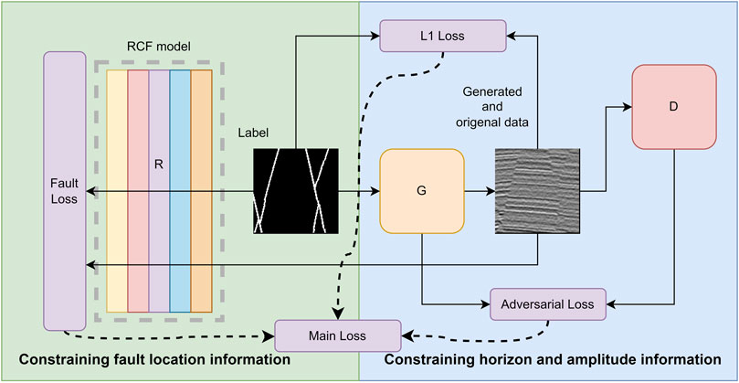
FIGURE 1. Fault2SeisGAN roadmap. Fault2SeisGAN transforms the fault labels by learning the mapping relationship between the seismic amplitude data distribution $p_{seis}\left(X|\theta \right)$ and location of the fault labels.

3 Network architecture

3.1 Fault2SeisGAN architecture

The network consists of two subnetworks, that is, generator and discriminator, and an Richer Convolutional Features for Edge Detection (RCF) module. The discriminator inputs are two two-dimensional (2D) vectors with a dimension of 256 × 256 × 1, representing amplitude data and their corresponding labels, respectively. The two vectors are concatenated in the feature dimension using a concatenate layer to obtain a 256 × 256 × 2 2D vector. A structure unit composed of convolution layers, normalization layers, and LeakyReLU activation function, called downsampling unit, can extract the features of the data and reduce the data size. Three downsampling units were combined to form an inverted pyramidal feature extraction structure, with number of features ranging from 2 to 64, 128, 256, and 512. The features are further extracted by two convolutional layers, and feature data with a size of (30, 30, 1) are obtained. To achieve stable network training, avoid local extrema, and appropriately reduce the discriminator performance, a dropout layer was added to the discriminator. Because this network uses the Wasserstein distance as the index to evaluate the network, the activation function was not used after the last drop.

The main architecture of the generator is a U-shaped network, which is divided into two parts: up- and downsampling. A connection layer is used to link the two parts such that the structural information can be transmitted, gradient dispersion caused by the deep network can be avoided, and the training difficulty can be reduced. We used transpose convolution, normalization, and ReLU activation functions to build an upsampling unit, which was combined with the previous downsampling unit to form the generator. In contrast to discriminators and other neural networks, GANs generally use the linear part of the convolutional layer without bias. In the downsampling part, eight downsampling units were used to sample the data to feature vectors with a size of (1, 1, 512). The upsampling part consists of seven upsampling units, each of which relates to the output result of the corresponding downsampling unit. The connected feature data are input to the next upsampling unit, and the output of the last downsampling unit is directly used as the input of the upsampling unit. After the U-shaped network, a transposed convolution layer is used to transform the feature data into the data domain, the number of feature layers becomes 1, and tanh is used to activate the feature data.

The RCF module adopts the conventional VGG16 structure to extract edge information features at multiple scales, compare the edge features of the generated data with those of the fault data, and calculate losses.

3.2 Objective function of the seismic constraint

Seismic amplitude data containing the fault consist of two parts. One is the “block” containing position and amplitude information, which constitutes the upper and lower wall of the fault. The other part is the location of the fault, that is, the “labels” that constrain these “blocks.’’ Note that we redesigned the GAN to separately constrain the two datasets.

3.2.1 Constraining horizon and amplitude information

To obtain data with horizon and amplitude characteristics like real seismic data, we did not use the random vector z as the seed of the generated data but adopted the more constrained fault location as the input. Based on this procedure, the network can still learn the mapping relationship between the fault label and seismic amplitude data distribution $p_g\left(z\left|\theta \right.\right)$ by training. Because fault location and seismic amplitude data have similar structures, the convolutional neural network (CNN) will constantly extract data features during forward propagation. When the network is relatively deep, the neural network can lose information and gradient. To maintain the 2D spatial structure of the data, we used a U-shaped CNN, utilized convolution to extract high-dimensional information of the data, and stepwise restored the data. Convolution and deconvolution constitute the decoder and encoder parts of the network. Shortcuts were added between the two parts of the network such that the output with original data structure information in the encoding process can be used to constrain the generation of the decoder. The network gradient can also be directly transferred to the following neural network through the direct connection layer, which improves the convergence speed of the network and reduces the training difficulty. The fault label is not only a marker of the fault location but also provides information about the boundaries between blocks, which is beneficial to the generation of amplitude data. The objective function of the network can be defined as follows:

The objective function can be divided into two parts. The first part is the objective function of the original GAN. It allows for the generator and discriminator to compete each other The second part is the L1 loss, which represents the similarity between the network input and output and can be defined as follows:

where represents the fault label data of the input generator and $G\left(x,z\right)$. represents the corresponding amplitude data generated by the generator. To reduce the calculation costs, the L1 norm is used to measure the difference between the two data. The difference between the input and generated amplitude is continuously determined to ensure the constraint of the label on the generated amplitude data.

3.2.2 Constraining fault location information

To generate amplitude data that are consistent with the location of the input fault, both types of data must be constrained. The location of a fault can be regarded as edge information of two disks. Both the fault location label and amplitude data contain such information, which can be extracted layer by layer, compared, and constrained. To extract the edge information, we introduced the RCF edge detection module, which is based on the deep neural network VGG16. The edge detection results were output for each level, and the results were accumulated according to a certain weight.

We input the fault location labels and corresponding generated data into the RCF detector R. By using the edge detector R, we obtained different levels of pixel-level edge detection effects. These edges correspond to fault information of different orders. Each point varies between 0 and 1, indicating the probability that the point is a fault. By using R, we compared R(x) and R[G(x)] of the fault edge information between fault labels and generated data:

In summary, the complete Loss function of the Fault2SeisGAN can be expressed as follows:

Where $\alpha$ and $\beta$ are the hyperparameters used to control the size of the constraint contribution of each part, which $\beta$ was set to 10, $\alpha$ was set to 1. Our objective function can be obtained as follows:

3.3 Stable network training

The GAN training is very unstable, especially with respect to the initial distribution and target distribution differences. The JS (Jensen–Shannon) divergence is a constant when the distribution between generated data and the real data is large, which cannot depict the distribution difference between the real data and generated data. These will case the vanishing gradient problem which could lead to generated data loss its diversity even become abnormal. To solve this problem, the Wasserstein distance (Cai et al., 2022) was used in this study instead of the JS divergence to improve the stability of the GAN and reduce the training difficulty. The Wasserstein distance is defined as:

where W is the degree of difference between the two distributions, and $\gamma \in \prod \left(p_r,p_g\right)$ is the set of all possible joint distributions of the $\left(p_r,p_g\right)$ distributions combined. For every possible joint distribution, $\gamma$ can sample $\left(x,y\right)\sim \gamma$ to obtain a sample x and y and calculate the distance between the pair of samples $\gamma$. Therefore, we can calculate the expected value of the sample with respect to the distance $‖x-y‖$ under the joint distribution ${\mathit{E}}_{\left(x,y\right)\sim \gamma }\left[‖x-y‖\right]$. The network structure used in this study is shown in Figure 2.

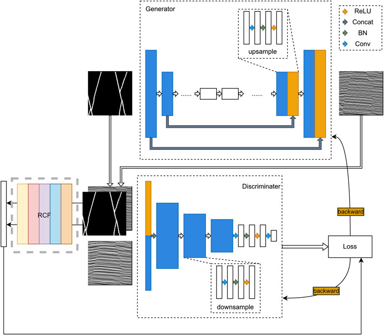
FIGURE 2. Architecture of Fault2SeisGAN. We input the fault location labels and corresponding generated data into the RCF detector R. By using the edge detector R, we obtained different levels of pixel-level edge detection effects.

4 Experiment

In this study, the TensorFlow2 framework was used to construct the neural network. Adam was used as the optimizer for the generator and discriminator. The learning rate was set to 2E-4 and 2E-5, and BETA1 was 0.5. The size of the dataset was (128, 128), and simple transformation, such as rotation, was performed to increase the number of datasets. A compute node with 12 cores and a 128 GB memory with a Tesla P100GPU computing card was used for the training. In total, 256000 samples were used as the dataset for this training, and the data were divided into training and test sets with a ratio of 7:3 and were run for a total of 200 epochs with a running time of 24 h. The samples in the test set were selected as input, and the proposed method was compared with the original GAN method with the added Wasserstein distance as well as the actual data. The results are shown in Figure 3.

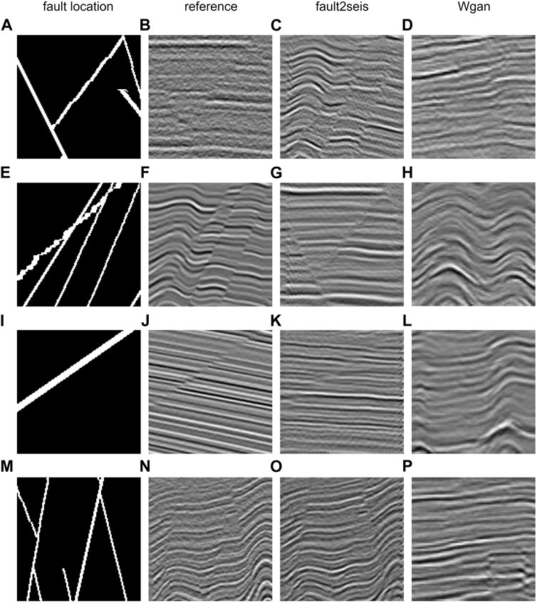
FIGURE 3. Comparison of the results using the test set. Fault2SeisGAN was used to generate amplitude data with labels (A, E, I, M). Compared with the test dataset (B, F, J, N), the Fault2SeisGAN’s results (C, G, K, O) has a similar structure, and fold features can also be learned by the network. Wgan’s results (D, H, L, P) as a comparison. The fault location is highly consistent with the labels.

If the Wasserstein distance is not added, the original GAN will fall into mode collapse and cannot generate data. In this study, the original GAN with the Wasserstein distance was used for comparison. Due to the addition of WGAN-GP (Wasserstein Generative Adversarial Network with Gradient Punishment), the samples generated with the original GAN are generally stable, and structural information, which is highly diverse, can be clearly obtained. However, due to the lack of constraints for fault labels, some of the generated data are not reasonable with respect to the structure, and some data even produce anomalies. These data can be screened, manually labeled, and then used as a training data set for the training of the segmentation network. In this study, the Fault2SeisGAN was used to generate amplitude data with labels. Compared with the test dataset, the Fault2SeisGAN has a similar structure, and fold features can also be learned by the network. The fault location is highly consistent with the labels. To sum up, amplitude data generated by the proposed method are consistent with the label information and share characteristics with actual data. Such data can be directly used for the training of other networks without manual annotation, which reduces labor costs.

GANs are flexible, but style transformation networks must have the same output and input data. The test and training set data have a certain similarity, which can be used to detect the generation ability of the network but cannot well describe it. Therefore, we used geometric transformation to randomly generate three-dimensional (3D) fault labels and then shuffled these labels and input them into the generator part for the prediction. Label data examples and their corresponding results are shown in Figure 3.

Compared with that of the data in test set, the quality of the amplitude data generated by our model according to the new fault label decreased, the continuity of the seismic event on both sides of the section weakened, and the seismic event became blurred. Although the generator can also produce some fold structures, the dip angle of the formation is gentler than before. Most fault locations correspond well to the amplitude data; only a few complex areas produce ambiguity. Thus, the characteristics of the generated amplitude data are more similar to the characteristics of the actual data. Figure 4 shows groups 1, 2, and 3, which are the predictions of two labels that are similar but not identical. The fault location is similar, but the generated amplitude data differ, indicating that the generator learns the data as well as their distribution.

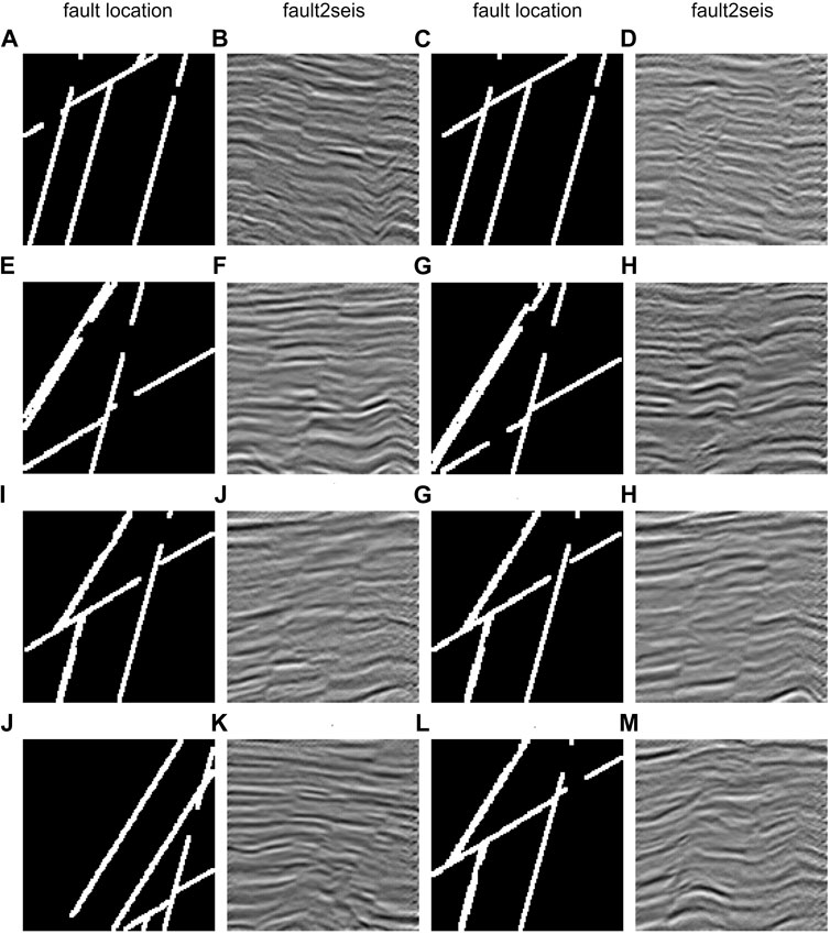
FIGURE 4. Random generation of fault locations (A, C, E, G, I, K, M, O) and the amplitude data generated by our model according to them. Although the generator can also produce some fold structures (B, F, J, N), the dip angle of the formation is gentler than before (D, H, L, P). Most fault locations correspond well to the amplitude data; only a few complex areas produce ambiguity.

4 Discussion

4.1 Effect of the expanded training data set on the performance of the fault identification network

To prove the effectiveness of the proposed method, we used the existing fault datasets and those generated by the proposed method to train the network model and predict the fault structure of real seismic data. In this study, 10,000 original datasets as well as a combination of the original data and 5,000 generated datasets were used for training. The results of the two datasets were compared and analyzed. All hyperparameters are shown in Table 1.

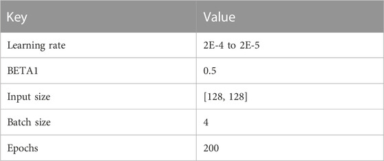
TABLE 1. Hyper-parameter.

U-Net is a network commonly used in CNNs to solve the segmentation problem. In recent years, it was mostly used to solve the fault identification problem in seismic exploration. In this study, the effectiveness of the sample generation by constructing a U-Net was verified. The U-Net structure used in this study is shown in Figure 5.

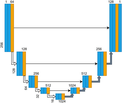
FIGURE 5. U-Net architecture used in this study. The U-Net have 4 downsample blocks and 5 upsample blocks. These corresponding blocks are connected by shortcut.

To prove the effectiveness of the proposed method, the original U-Net was used as the fault identification network. The network consists of five coding and four decoding modules with Concat links and a separate convolution module before the network output. Therefore, the input and output of the network have the same size and output a specific number of channels. Each coding module consists of two convolution layers with 3 × 3 convolution kernels and a normalization layer. ReLu is used as the activation function. The decoding module uses a convolutional layer and an upsampling layer, which were normalized using batch normalization and activated using ReLu.

In this study, a data random scaling mechanism was added after the data input, which increases the range of the network and improves the recognition accuracy of the actual data.

We used 10000 fault datasets and 5,000 datasets generated by the proposed method as training datasets for the comparison and divided the experiment into two groups: 1) 10000 original fault datasets and 2) a mixture of both datasets.

We tested the performance of the two trained neural networks using a set of real data, and the results are shown in Figure 6. In Figure 6A we can see that there are lots of faults and most of them are recognized in Figure 6B. However, there still miss some faults and occurs discontinuity identification in the middle and the left side. All 4 faults in the middle were identified very precisely. In the left part, although some of the faults are also identified, the continuity of faults is very poor. In the left most part, multiple faults are intersected and only the most obvious fault patterns are identified in network 1). In contrast, Figure 6C do better in the middle of the seismic data profile where the seismic event is not clearly and continuity. The results show that the training of the dataset with the proposed method is effective and improves the performance of the deep neural network with respect to the fault recognition.

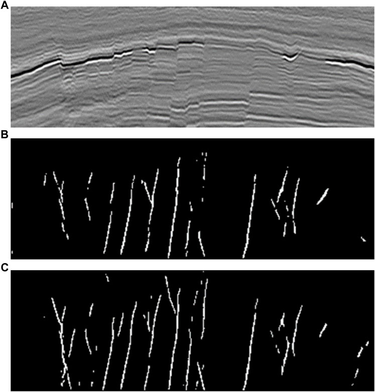
FIGURE 6. Fault (A) identification results for different datasets. there still miss a lot of faults and occurs discontinuity identification in the middle and the left side (B). In contrast, (C) do batter in the middle of the seismic data profile where the seismic event is not clearly and continuity.

5 Conclusion

In this study, we propose an end-to-end training data set expansion network, that is, Fault2SeisGAN. The network is based on GAN technology, which extends limited labeled datasets to improve the performance of other neural networks. In this method, the Seis Loss is used to constrain the horizon and amplitude information, RCF and Fault Loss are combined to constrain the fault location information, and the Wasserstein distance is added to stabilize the network training. Based on the use of the Fault2SeisGAN, existing data can be extended, new fault datasets can be obtained, and the performance of the fault identification network can be improved. Based on the use of the original U-Net for training in the last part of this study, we obtained better results compared with those obtained with the utilization of the network that was only trained with the original dataset, which proves the effectiveness and practicability of the proposed method. Our method solves the shortage of training data set problem caused by the application of deep learning technology in seismology to a certain extent, improves the performance of neural networks, and promotes the development of deep learning technology in seismology.

Our method also has some limitations. Compared to traditional deep learning methods, although our method requires fewer real data with labels to build the training dataset, however, it is also very difficult to collect real data with labels. The signal-to-noise ratio of the data used in this article is relatively high, and the impact of low signal-to-noise ratios and other more complex cases on the results needs to be further studied and discussed.

The focus of this study was placed on generating paired 2D datasets with fault amplitudes. In future research, the generation of 3D and multi-attribute data as well as data feature control should be considered.

Data availability statement

The raw data supporting the conclusion of this article will be made available by the authors, without undue reservation.

Author contributions

Conceptualization, RD and SZ; Methodology, SZ; Writing—original draft, SZ; Writing—review and editing, TH, YL, JZ, and LZ. All authors have read and agreed to the published version of the manuscript.

Funding

Major Research Plan on West-Pacific Earth System Multispheric Interactions (Grant No. 92058213), Shandong Provincial Natural Science Foundation, China (Grant No. ZR2022QD087), National Natural Science Foundation of China (Grant No. 41676039 and 41930535).

Conflict of interest

The authors declare that the research was conducted in the absence of any commercial or financial relationships that could be construed as a potential conflict of interest.

Publisher’s note

All claims expressed in this article are solely those of the authors and do not necessarily represent those of their affiliated organizations, or those of the publisher, the editors and the reviewers. Any product that may be evaluated in this article, or claim that may be made by its manufacturer, is not guaranteed or endorsed by the publisher.

References

Adler, A., Araya-Polo, M., and Poggio, T. (2019). “Deep recurrent architectures for seismic tomography,” in 81st EAGE conference and exhibition 2019 (London, UK: European Association of Geoscientists & Engineers), 1–5. doi:10.3997/2214-4609.201901512
Araya-Polo, M., Adler, A., Farris, S., and Jennings, J. (2020). “Fast and accurate seismic tomography via deep learning,” in Deep learning: Algorithms and applications studies in computational intelligence Editors W. Pedrycz,, and S.-M. Chen (Cham: Springer International Publishing), 129–156. doi:10.1007/978-3-030-31760-7_5
Araya-Polo, M., Jennings, J., Adler, A., and Dahlke, T. (2018). Deep-learning tomography. Lead. Edge 37, 58–66. doi:10.1190/tle37010058.1
Cai, A., Qiu, H., and Niu, F. (2022). Semi-supervised surface wave tomography with Wasserstein cycle-consistent GAN: Method and application to southern California plate boundary region. J. Geophys. Res. Solid Earth 127, e2021JB023598. doi:10.1029/2021JB023598
Cunha, A., Pochet, A., Lopes, H., and Gattass, M. (2020). Seismic fault detection in real data using transfer learning from a convolutional neural network pre-trained with synthetic seismic data. Comput. Geosci. 135, 104344. doi:10.1016/j.cageo.2019.104344
Goodfellow, I. J., Pouget-Abadie, J., Mirza, M., Xu, B., Warde-Farley, D., Ozair, S., et al. (2014). Generative adversarial networks. ArXiv14062661 Cs stat. Available at: http://arxiv.org/abs/1406.2661 (Accessed September 23, 2021).
Herrmann, F. J., and Hennenfent, G. (2008). Non-parametric seismic data recovery with curvelet frames. Geophys. J. Int. 173 (1), 233–248. doi:10.1111/j.1365-246X.2007.03698.x
Hu, L., Zheng, X., Duan, Y., Yan, X., Hu, Y., and Zhang, X. (2019). First-arrival picking with a U-net convolutional network. Geophysics 84, U45–U57. doi:10.1190/geo2018-0688.1
Mandelli, S., Borra, F., Lipari, V., Bestagini, P., Sarti, A., and Tubaro, S. (2018). “Seismic data interpolation through convolutional autoencoder,” in SEG technical program expanded abstracts 2018 (Anaheim, California: Society of Exploration Geophysicists), 4101–4105.
Wang, B., Zhang, N., Lu, W., and Wang, J. (2019). Deep-learning-based seismic data interpolation: A preliminary result. Geophysics 84, V11–V20. doi:10.1190/geo2017-0495.1
Wang, F., Song, X., and Li, J. (2022). Deep learning-based H-κ method (HkNet) for estimating crustal thickness and vp/vs ratio from receiver functions. J. Geophys. Res. Solid Earth 127, e2022JB023944. doi:10.1029/2022JB023944
Wang, Y., Wang, B., Tu, N., and Geng, J. (2020). Seismic trace interpolation for irregularly spatial sampled data using convolutional autoencoder. Geophysics 85, V119–V130. doi:10.1190/geo2018-0699.1
Wu, H., Zhang, B., Li, F., and Liu, N. (2019a). Semiautomatic first-arrival picking of microseismic events by using the pixel-wise convolutional image segmentation method. Geophysics 84, V143–V155. doi:10.1190/geo2018-0389.1
Wu, H., Zhang, B., Lin, T., Li, F., and Liu, N. (2019b). White noise attenuation of seismic trace by integrating variational mode decomposition with convolutional neural network. Geophysics 84, V307–V317. doi:10.1190/geo2018-0635.1
Wu, X., Geng, Z., Shi, Y., Pham, N., Fomel, S., and Caumon, G. (2020). Building realistic structure models to train convolutional neural networks for seismic structural interpretation. Geophysics 85, WA27–WA39. doi:10.1190/geo2019-0375.1
Wu, X., Liang, L., Shi, Y., and Fomel, S. (2019c). FaultSeg3D: Using synthetic data sets to train an end-to-end convolutional neural network for 3D seismic fault segmentation. Geophysics 84, IM35–IM45. doi:10.1190/geo2018-0646.1
Wu, X., Shi, Y., Fomel, S., Liang, L., Zhang, Q., and Yusifov, A. Z. (2019d). FaultNet3D: Predicting fault probabilities, strikes, and dips with a single convolutional neural network. IEEE Trans. Geosci. Remote Sens. 57, 9138–9155. doi:10.1109/tgrs.2019.2925003
Yang, J., Ding, R.-W., Wang, H.-Y., Lin, N.-T., Zhao, L.-H., Zhao, S., et al. (2022). Intelligent identification method and application of seismic faults based on a balanced classification network. Appl. Geophys. 2022 , 1–12. doi:10.1007/s11770-022-0976-9
Yu, S., and Ma, J. (2021). Deep learning for Geophysics: Current and future trends. Rev. Geophys. 59, e2021RG000742. doi:10.1029/2021rg000742
Yu, S., Ma, J., and Wang, W. (2019). Deep learning for denoising. Geophysics 84, V333–V350. doi:10.1190/geo2018-0668.1
Yuan, P., Wang, S., Hu, W., Wu, X., Chen, J., and Van Nguyen, H. (2020). A robust first-arrival picking workflow using convolutional and recurrent neural networks. Geophysics 85, U109–U119. doi:10.1190/geo2019-0437.1
Zhang, K., Zuo, W., Chen, Y., Meng, D., and Zhang, L. (2017). Beyond a Gaussian denoiser: Residual learning of deep CNN for image denoising. IEEE Trans. Image Process. 26, 3142–3155. doi:10.1109/tip.2017.2662206
Keywords: deep learning, fault recognition, generative adversarial network, training dataset construction, loss function, data analyse
Citation: Zhao S, Ding R, Han T, Liu Y, Zhang J and Zhao L (2023) Fault2SeisGAN: A method for the expansion of fault datasets based on generative adversarial networks. Front. Earth Sci. 11:1091803. doi: 10.3389/feart.2023.1091803
Received: 07 November 2022; Accepted: 11 January 2023;
Published: 20 January 2023.
Edited by:
Tariq Alkhalifah, King Abdullah University of Science and Technology, Saudi ArabiaReviewed by:
Keyvan Khayer, Shahrood University of Technology, IranAmin Roshandel Kahoo, Shahrood University of Technology, Iran
Mohammad Radad, Shahrood University of Technology, Iran
Copyright © 2023 Zhao, Ding, Han, Liu, Zhang and Zhao. This is an open-access article distributed under the terms of the Creative Commons Attribution License (CC BY). The use, distribution or reproduction in other forums is permitted, provided the original author(s) and the copyright owner(s) are credited and that the original publication in this journal is cited, in accordance with accepted academic practice. No use, distribution or reproduction is permitted which does not comply with these terms.
*Correspondence: Renwei Ding, dingrenwei@126.com