Eocene-Oligocene southwest Pacific Ocean paleoceanography new insights from foraminifera chemistry (DSDP site 277, Campbell Plateau)

1 Introduction

Facing ongoing global warming, understanding the feedbacks driving the Earth’s climate is one of the greatest challenges of Earth sciences. As a pivotal period marking the transition from a greenhouse to the modern icehouse world, the Eocene-Oligocene interval has been studied for decades to identify and decipher the climate mechanisms driving this cooling (e.g., Zachos et al., 2001; Hutchinson et al., 2021) (Figure 1). Today, it is generally accepted that a reduction in atmospheric pCO₂ played a major role in this transition, resulting in the cooling and then glaciation (e.g., DeConto and Pollard, 2003; Pagani et al., 2011; Ladant et al., 2014; Kennedy-Asser et al., 2020; Hutchinson et al., 2021). However, ocean dynamics also play a key role in Earth’s climate. Indeed, oceanic circulation controls global heat transfers while oceanic primary productivity and the associated biological pump is a major atmospheric CO₂ sink (e.g., Jovane et al., 2009; Goldner et al., 2014; Elsworth et al., 2017; Toumoulin et al., 2020; Zhang et al., 2020; Sauermilch et al., 2021). Hence, constraining the evolution of oceanic circulation and the chemistry of different water masses during the Eocene-Oligocene transitions is fundamental for a better understanding of the Earth’s climate changes.

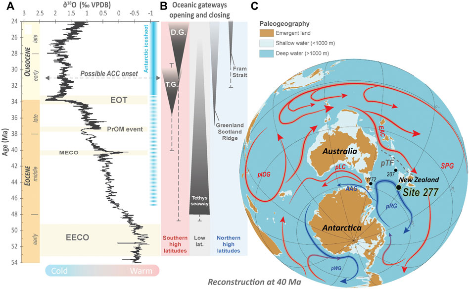
FIGURE 1. (A) Temporal evolution of the global benthic foraminifera δ¹⁸O records and main climate events along the Eocene-Oligocene interval (from the GTS2020 by Gradstein (2020)). Possible occurrences of Antarctica ice-cap are also represented after Zachos et al. (2001). Possible ACC (Antarctic Circumpolar Current) onset is from Scher et al. (2015) and Hodel et al. (2021). (B) Opening and closing timing of main oceanic gateways during the Eocene-Oligocene (from Straume et al., 2020). (C) Paleogeographic and paleobathymetric representation of the southern hemisphere at the Oligocene, ca. 30 Ma (paleobathymetric data from Straume et al., 2020 and model built using the GPlate software, Müller et al., 2018). Paleocurrents are represented based on Nelson and Cooke, (2001), Huber et al. (2004), Stickley et al. (2004), Bijl et al. (2009, Sijp et al. (2011); Pascher et al. (2015), Hines et al. (2017), Houben et al. (2019); Ladant et al. (2020), Straume et al. (2020), Hodel et al. (2021), Shepherd et al. (2021) and Sauermilch et al. (2021). Abbreviations: EOT, Eocene-Oligocene Transition; PrOM event, Priabonian Oxygen isotope Maximum event; MECO, Middle Eocene Climate Optimum; EECO, Early Eocene Climate Optimum; T.G, Tasmanian Gateway; D.G, Drake Passage Gateway; pIOG, proto-Indian Ocean Gyre; pLC, proto-Leeuwin current; pWG: proto-Weddell Gyre; pRG, proto-Ross Gyre; ACC, Antarctic Circumpolar Current; pTF, proto-Tasman Front; EAC, East Australian Current; SPG, South Pacific Gyre.

Antarctica and the surrounding Southern Ocean have been a significant focus of the last decades given their high sensitivity to cooling and glaciation during the Eocene-Oligocene (e.g., Kennett et al., 1975; Nelson and Cooke, 2001; Zachos et al., 2001; Stickley et al., 2004; Bijl et al., 2009; , 2021; Bohaty et al., 2012; Hollis et al., 2012, 2015; Scher et al., 2014, 2015; Pascher et al., 2015; Hodel et al., 2021; Sauermilch et al., 2021; Shepherd et al., 2021). Located at the outlet of the Tasmanian gateway, the DSDP Site 277 on the Campbell Plateau (Figure 1) was drilled specifically to investigate the role played by the Antarctic Circumpolar Current (ACC) in the thermal isolation of Antarctica from tropical heat fluxes (e.g., Kennett et al., 1975) (Figure 1). There is significant evidence that the development of the ACC played a major role in cooling and keeping Antarctica cool (e.g., Kennett, 1977; Kennett and Exon, 2004; Sauermilch et al., 2019, 2021). In this study, we investigate the role that other currents such as the proto-East Australian Current and the proto-Ross gyre (e.g., Nelson and Cooke, 2001; Bijl et al., 2009; Pascher et al., 2015; Sauermilch et al., 2021; Shepherd et al., 2021) played on the ocean heat fluxes, ocean redox state and primary productivity during the Eocene-Oligocene cooling.

Here, we investigate the physico-chemical properties of the southwest Pacific water masses recorded at Site 277 to better decipher the high latitude Southern Ocean dynamics during the Eocene-Oligocene cooling. Site 277 (52°13.43'S; 166°11.48'E) is located on the Campbell Plateau, South of New Zealand, between Auckland and Campbell Islands. The site was drilled to better understand the paleoceanographic history of the region related to long-term oceanic structural changes and Antarctic glaciation (Kennett et al., 1975). It is characterized by continuous sedimentation from the middle Paleocene to the late Oligocene (Kennett et al., 1975). The Eocene-Oligocene section of the Site 277, is composed of two main lithological units: Unit 2 (13 - 246 mbsf) and Unit 3 (246–454) mbsf. Unit 2 is a nannofossil ooze containing glauconite, radiolaria, foraminifera, minor amounts of diatoms and sponge spicules. Unit 3 only differs by the fact that siliceous fossils are poorly preserved and less abundant and by the occurrence of chert nodules (Hollis et al., 1997). Site 277 is thus characterized by a very uniform and mainly biogenic Eocene-Oligocene sedimentary record, with minor detrital materials (Kennett et al., 1975). It, therefore, constitutes an ideal target for paleoceanographic studies dealing with marine biocarbonates. The modern water depth at Site 277 is 1232 m below sea level. Its paleodepth during the Eocene-Oligocene interval is estimated to be 1,000–1,500 m, well above the lysocline at lower to middle bathyal water depths since the Paleocene (Hollis et al., 1997).

We applied several chemical proxies to planktic and benthic foraminifera from Site 277: (1) Mg/Ca and δ¹⁸O ratios to infer seawater temperature and ice-volume evolution, (2) Ce anomaly (Ce/Ce*) as a seawater redox proxy, (3) U/Ca ratio as a sedimentary redox proxy, and (4) the δ¹³C as a potential paleoproductivity proxy in combination with sedimentation rates (e.g., Katz et al., 2010 for a review, Chase et al., 2001; Boiteau et al., 2012; Chen et al., 2017; Remmelzwaal et al., 2019; Hodel et al., 2021). All these proxies were analyzed for both benthic (mixed Gyroidinoides sp. and Cibicidoides sp.) and planktonic foraminifera (Subbotina sp.) from Site 277 to decipher physico-chemical features of bottom and surface water. These results provide new insights to better constrain southwest Pacific Ocean circulation, associated heat transfer, ocean and sedimentary redox evolution as well as paleoproductivity nearby Antarctica across the Eocene-Oligocene cooling.

2 Materials and methods

2.1 Foraminifera separation and cleaning

Based on the detailed core descriptions of Kennett et al. (1975), 27 sediment samples were selected for foraminifera analysis. Each sample was resuspended into Milli-Q water, ultrasonicated and sieved at 200 µm. Each fraction was dried for 48 h in an oven at 50°C. Then, planktonic (Subbotina sp., thermocline dwellers, e.g., Pearson et al., 2006; Hollis et al., 2012; Pascher et al., 2015) and benthic foraminifera (Cibicidoides sp. and Gyroidinoides sp.) were hand-picked separately under a stereo microscope. We only selected entire, clean and well-preserved specimens devoid of visible recrystallization, clay aggregates and oxyhydroxide patches (Figure 3). Each planktic and benthic foraminifera sample was then cleaned and digested in a clean laboratory following the procedure of Hodel et al. (2021). Foraminifera tests cleaning method consists of several ultrasonications in MQ water (Molina-Kescher et al., 2014; Osborne et al., 2017; Hodel et al., 2021) rather than the oxidizing-reducing cleaning of Barker et al. (2003). This allows the preservation of secondary coatings hosting the sedimentary redox signal (foraminiferal U/Ca ratio evolutions) that we investigate further in this contribution. For each sample, back-scattered electrons (BSE) images of foraminifera tests (and residues after chemical treatment) were obtained using a JEOL JSM-6360LV electron microscope operating at 20 kV at the Observatoire Midi-Pyrénées (PANGEE instrumental Platform, Toulouse, France).

2.2 Elemental chemistry

Major and trace element concentrations of each foraminiferal fraction were obtained through the all-in-one procedure developed in Hodel et al. (2021). Cleaned foraminifera fractions were dissolved into 1 ml of a 0.5 N acetic acid solution. Then, major and trace element concentrations were measured using a Thermo Scientific Element XR HR-ICP-MS at the Observatoire Midi-Pyrénées (Toulouse, France) (see Hodel et al., 2021 for more details). The oxide interferences (BaO+ on Nd+ and Eu+, LREE on MREE, and MREE on HREE, see table in Supplementary Material S1) were then corrected. Oxide production rate was determined based on the Cal-S standard material (Calcite, Yeghicheyan et al., 2003). The precision and accuracy of ICP-MS analyses were assessed by measuring the Cal-S standard. Element concentrations of all analyzed foraminiferal fractions are available in Supplementary data.

2.3 Oxygen and carbon isotope ratio analysis

Stable isotope analyses were performed at the ISTeP Laboratory (Sorbonne Université, Paris, France) using a Kiel IV carbonate automatic device coupled with a DELTA V Advantage isotope ratio mass spectrometer. Foraminiferal oxygen and carbon isotope compositions were obtained by measuring the oxygen and carbon stable isotopes of carbon dioxide generated by the dissolution of planktonic and benthic foraminifera samples using anhydrous orthophosphoric acid at 70°C. Isotope values are reported in conventional delta (δ) notation as per mil (‰) deviations of the isotopic ratios (¹⁸O/¹⁶O) calculated to the VPDB scale. Accuracy and precision of 0.08‰ (1σ) for both O and C isotopes were determined by repeated analyses of an internal Carrara marble standard, calibrated against the international standard NBS-19. Results of all the foraminiferal δ¹⁸O and δ¹³C analyses of this study are available in Supplementary data.

2.4 Paleotemperature calculation

2.4.1 Mg/Ca temperatures

Mg/Ca-derived paleotemperatures were calculated using the latest power law relationship established to describe foraminiferal Mg/Ca ratio and temperature covariations (Hollis et al., 2015; Hines et al., 2017 and reference therein, Eq. 1). The latter is an update of the exponential relationship of Lear et al. (2002) to better fit past seawater Mg/Ca ratios (Mg/Ca_sw).

In this study, we used a value of 1.6 mol.mol⁻¹ for the Mg/Ca ratio of seawater at the time of test crystallization (i.e., Mg/Ca_sw^t=t, Stanley and Hardie, 1998; Evans and Müller, 2012; Hollis et al., 2015; Hines et al., 2017). Possible variations of this value along the studied interval are further discussed (see part 4.2.4). The Mg/Ca ratio of modern seawater (Mg/Ca_sw^t=0) has been fixed at 5.17 mol.mol⁻¹ (Stanley and Hardie, 1998; Evans and Müller, 2012). For surface seawater temperatures (SST), we used the general calibration of Anand et al. (2003), which is based on nine planktonic species (A = 0.09 and B = 0.38) and an H value of 0.29 (Creech et al., 2010; Hollis et al., 2012). For seafloor temperatures (SFTs), we used the calibration of Lear et al. (2002) based on three Cibicidoides species (A = 0.109 and B = 0.867) and an H value of 0.16 (Burgess et al., 2008). Errors on calculated temperatures were determined by considering the relative standard deviation (RSD) on Mg and Ca concentrations of 1.03% and 1.14% on average, respectively, as well as the calibration error of ±1.6°C on the multi-species calibrations established by Lear et al. (2002) and Anand et al. (2003). The cumulative error calculated provides upper and lower uncertainties (±1.62°C on average). All the paleotemperatures calculated based on Mg/Ca molar ratios are available in Supplementary data.

2.4.2 δ¹⁸O temperatures

δ¹⁸O-derived paleotemperatures were calculated using the equation of Kim and O'Neil (1997) for both benthic and planktonic foraminifera (Eq. 2):

where δ¹⁸O_M is the measured value and δ¹⁸O_sw the seawater value. Here, δ¹⁸O_sw is fixed to −1.23‰, including an ice-volume component of −0.96‰ (Zachos et al., 1994) and a SMOW to VPDB correction of −0.27‰ (Kim and O’Neil, 1997). We fixed the ice-volume component because the evolution of global continental ice volume along the Eocene-Oligocene interval remains unconstrained. This likely induces a bias on calculated temperatures, notably across and after the Eocene-Oligocene Transition (EOT), which is debated further (see part 4.2.4.). Planktonic δ¹⁸O values were corrected for paleolatitude (correction of −0.23‰ for ca. 65 °S, Zachos et al., 1994). We also applied a correction of +0.28‰ for benthic species (Katz et al., 2003; Hollis et al., 2015). All the δ¹⁸O-derived paleotemperatures are available in Supplementary data.

2.4 Age model and sedimentation rate calculations

Age estimations for each sample have been calculated using the biochronological data from Hollis et al. (1997) for Site 277 and updated with the recently published nannofossil data of Shepherd et al. (2021) for the Eocene interval. Data of Hollis et al. (1997) were recalibrated to the GTS 2012 (Gradstein et al., 2012) (see Supplementary Material S2). We used the changepoint (Killick and Eckley, 2014) and segmented (Vito and Muggeo, 2003) packages implemented on the R software (R Development Core Team, 2019) to identify statistically robust trends of sedimentation rate fitting with linear regressions and to calculate the absolute age of each selected sample (Figure 2) (see Hodel et al., 2021 for a similar approach). The 95% confidence interval of these regressions (jack-knife R script) defined uncertainties on obtained ages (from ± 0.10 to ± 0.6 Ma, Figure 2). The calculated ages with their associated uncertainties are reported in Supplementary Material S2.

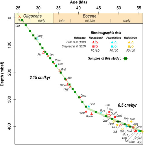
FIGURE 2. Age model for selected samples (green squares) from the DSDP Leg 29 Site 277. Calibrations are based on the integrated biostratigraphic study of Hollis et al. (1997) and the recent study of Shepherd et al. (2021) for the Eocene Data and taxa abbreviations shown in Supplementary data 2. Regressions are computed using the packages changepoint (Killick and Eckley, 2014) and segmented (Vito and Muggeo, 2003) on the R software (R Development Core Team, 2019). Uncertainties (represented in shaded green) correspond to the 95% confidence interval of regressions.

3 Results

3.1 Sample ages

Calculated ages of our samples range from 55.4 ± 0.6 Ma to 26.0 ± 0.1 Ma. Our sampling frequency resolution is between 0.5 and 1.2 Ma from 26.0 to 41.8 Ma and between 1.3 and 2.6 Ma from 44.3 to 55.4 Ma. Our statistical approach allowed us to identify two main sedimentation regimes (in line with Hollis et al., 1997), namely a sedimentation rate of ∼ 0.5 cm/kyr between 55.4 ± 0.6 Ma and 41.8 ± 0.1 Ma and of ∼ 2.15 cm/kyr between 41.8 ± 0.1 Ma and 26.0 ± 0.1 Ma (Figure 2). Shepherd et al. (2021) recently mentioned two hiatuses at Site 277 in the early and middle Eocene that we do not observe with our statistical model. This likely relies on the fact that our linear regressions are based on several biostratigraphic data points. It results in a slightly less resolved but statistically more robust age model. However, it is worth noting that the calculated uncertainties of our ages take into account the poor distribution of the biostratigraphic markers for this time interval. Thus, the effect of these possible hiatuses on our ages is encompassed in the error bars.

3.2 Scanning electron microscopy imaging: Test preservation

Scanning electron microscopy (SEM) observations (Figure 3) have been used to assess the preservation state of benthic and planktonic foraminifera. As evidenced by previous studies (e.g., Hollis et al., 2015; Shepherd et al., 2021), planktonic foraminifera from Site 277 are characterized by a “frosty” texture (Sexton et al., 2006), resulting from minor authigenic calcite recrystallization after the deposition of the test on the seafloor and/or during their sinking through the water column (Figures 3A,B). Benthic foraminifera show a smoother texture without visible secondary calcite recrystallization. SEM observations of the residues after the foraminifera test acid dissolution (0.5 M CH₃COOH) indicate that only calcite has been dissolved, indicating minimal contamination by detrital material (e.g., clay mineral, quartz, mica and feldspar grains) or early-diagenetic mineral such as pyrite (Figures 3E,F).

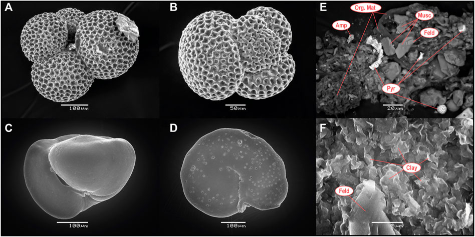
FIGURE 3. Back-scattered electron (BSE) SEM microphotographs of (A,B) planktonic foraminifera (Subbotina sp.) and (C,D) benthic foraminifera (Gyroidinoides sp. and Cibicidoides sp., respectively) from the DSDP Site 277. (E) and (F) are examples of residues remaining after 0.5 M CH₃COOH tests dissolution. Abbreviations stand for Pyr, pyrite; Org. Mat, organic matter; Musc, muscovite; Amp, amphibole; Feld, feldspar.

3.3 Foraminiferal Rare Earth Element concentrations

All analyzed foraminifera show smooth seawater-like PAAS (Post Archean Australian Shales) normalized REE element patterns (Figures 4A,B) characterized by: 1) a depletion in LREE (Light Rare Earth Elements) compared to HREE (Heavy Rare Earth Elements, (Pr/Yb)_N ratios ranging from 0.27 to 0.57 and 0.29 to 0.60 for benthic and planktonic foraminifera, respectively), 2) a marked negative Ce anomaly (Ce/Ce* = Ce_N/(Pr_N x (Pr_N/Nd_N)), ranging from 0.31 to 0.90 and 0.29 to 0.92 for benthic and planktonic foraminifera, respectively) and 3) a pronounced positive La anomaly (La/La*= La_N/(Pr_N x (Pr_N/Nd_N)²) ranging from 1.58 to 2.48 and 1.60 to 2.23 for benthic and planktonic foraminifera, respectively). All these features are characteristic of modern seawater chemistry (e.g., Elderheld and Greaves, 1982; Elderfield, 1988; Grenier et al., 2013; Jeandel et al., 2013; Hathorne et al., 2014; Deng et al., 2017). Interestingly, temporal evolutions of the Ce/Ce* values display clear stepwise tendencies (Figure 4C). From 55.4 Ma to 41.8 Ma, Ce/Ce* values are high and fluctuate between 0.67 to 0.90 and 0.69 to 0.92 for benthic and planktonic foraminifera, respectively. From 41.8 Ma onward, Ce/Ce* values decrease considerably in both benthic and planktonic species in a series of steps. First, Ce/Ce* values decrease from 0.88 at 41.8 Ma to 0.62 at 39.1 Ma and stabilize ca. 0.62 from 39.1 to 35.6 Ma. A second marked drop occurs between 35.6 and 34.4 Ma down to ca. 0.47. Finally, a third major drop of the Ce/Ce* values down to ca. 0.30 is noticeable between 31.8 and 31.0 Ma. Then the Ce anomaly remains constant until 26.0 Ma.

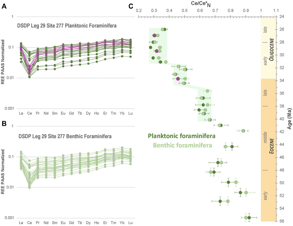
FIGURE 4. (A,B) PAAS normalized REE spectrum of the studied (A) planktonic (Subbotina sp.) and (B) benthic foraminifera (Cibicidoides sp. and Gyroidinoides sp.) tests from the DSDP Site 277. PAAS normalizing values are from Barth et al. (2000) with Tm from Kamber et al. (2005). (C) Evolution of the negative Ce anomaly (Ce/Ce* ratio) along the Eocene-Oligocene interval. The samples highlighted in pink are the three samples slightly above the contamination threshold for Al/Ca and Sr/Ca molar ratios (see Figure 5).

3.4 Foraminiferal major and traces element concentrations

3.4.1 Contamination evaluation

In addition to SEM observations and REE concentrations, Al/Ca vs. Mg/Ca and Sr/Ca vs. Mg/Ca diagrams can be used in chemical studies on foraminifera to monitor potential contaminations (e.g., Hollis et al., 2015; Osborne et al., 2017; Henehan et al., 2020; Hodel et al., 2021). In their laser ablation study, Hollis et al. (2015) calculated threshold values in such diagrams to discard samples with Mg/Ca-temperatures possibly biased by more than 1°C by detrital silicates, early-diagenetic (coatings) and/or recrystallization processes. In our study, all samples show low Al/Ca ratio with values ranging from 0.005 to 0.07 mmol.mol⁻¹ and 0.008–0.166 mmol.mol⁻¹ for benthic and planktonic foraminifera, respectively (Figure 5A). These values are well below the contamination threshold established by Hollis et al. (2015), namely Al/Ca > 2 mmol.mol⁻¹ (Figure 5A). Only one sample (26.9 Ma) displays Al/Ca ratio above the threshold value of 0.140 fixed by Rae et al. (2011) and Henehan et al. (2020) for potential clay contamination (Figure 5A). With Sr/Ca ratio ranging from 0.92 to 1.38 and 0.90 to 1.67 for benthic and planktonic foraminifera, respectively, our data also lie within the range of 0.8–1.6 mmol.mol⁻¹ established by Hollis et al. (2015) for acceptable values, except for two planktonic foraminifera samples showing ratios of 1.62 and 1.67. These two samples and the sample with Al/Ca ratio > 0.140 were discarded and not included in the discussion. They are circled in pink in the figures.

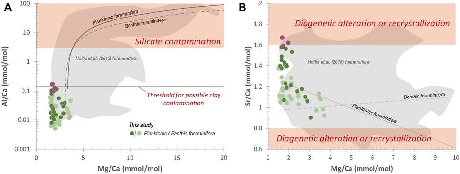
FIGURE 5. (A) Cross-plots of Al/Ca vs Mg/Ca ratios and (B) Sr/Ca vs Mg/Ca ratios measured in the foraminiferal fractions. Screening limits in shaded red are from Hollis et al. (2015). Another Al/Ca ratio threshold for potential clay contamination from Rae et al. (2011) and Henehan et al. (2020) is represented (red line in a). Shaded grey domains and grey trend lines represent the LA-ICP-MS data of Hollis et al. (2015) on benthic and planktonic foraminifera from the Site 277 for comparison. The samples highlighted in pink are the three samples slightly above the contamination threshold for Al/Ca and Sr/Ca molar ratios.

3.4.2 Mg/Ca ratio

Mg/Ca ratio ranges between 1.51 and 3.69 mmol.mol⁻¹ and 1.58–3.06 mmol.mol⁻¹ for benthic and planktonic foraminifera, respectively (Figure 6A). From 55.4 Ma to 46.8 Ma, both benthic and planktonic foraminifera show high Mg/Ca ratio, varying between 3.32 and 3.69 and 2.41 and 3.06, respectively. Mg/Ca ratio is rather stable during this time interval for benthic foraminifera, while it slightly decreases in the planktonic record. Then, the Mg/Ca ratio drops down to much lower values of 2.04 and 1.89 in the benthic and planktonic foraminiferal fractions, respectively at 44.3 Ma. From 44.3 Ma onwards, the Mg/Ca ratio of both benthic and planktonic foraminifera is more stable with values of 1.51–2.14 and 1.66 to 2.16 for benthic and planktonic foraminifera, respectively, except for some peaks in the benthic record at 41.0 Ma (Mg/Ca = 2.47), 39.1 Ma (Mg/Ca = 2.46) and 32.2 Ma (Mg/Ca = 2.44).

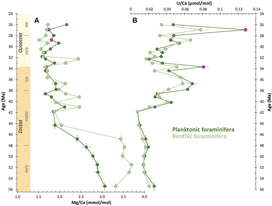
FIGURE 6. Temporal evolution of (A) Mg/Ca molar ratios (in mmol.mol⁻¹) and (B) U/Ca molar ratios (in µmol.mol⁻¹). Samples highlighted in pink are the three samples slightly above the contamination threshold for Al/Ca and Sr/Ca molar ratios (see Figure 5).

3.4.3 U/Ca ratio

Foraminiferal U/Ca ratio ranges from 0.007 to 0.078 μmol.mol⁻¹ and 0.007–0.128 μmol.mol⁻¹ for benthic and planktonic foraminifera, respectively (Figure 6C). U/Ca ratio is very low and stable from 55.4 to 41.8 Ma (from 0.007 to 0.020 μmol.mol⁻¹ and 0.007–0.026 μmol.mol⁻¹ for benthic and planktonic foraminifera, respectively). Then, it rapidly increases from 41.8 Ma onwards and reaches values of 0.058 and 0.068 μmol.mol⁻¹ at 36.7 Ma. Further on, the U/Ca ratio decreases down to values of 0.017 and 0.020 μmol.mol⁻¹ at 32.2 Ma in benthic and planktonic foraminifera, respectively. Finally, the U/Ca ratio increases again, more gradually, from 32.2 Ma to 26.0 Ma.

3.5 Oxygen and carbon isotope compositions

Foraminiferal δ¹⁸O values range from -0.96 to +2.22‰ for benthic species and between −1.30 and +1.64‰ for planktonic species (Figure 7A). Overall, the benthic and planktonic δ¹⁸O signals show a similar evolution, despite average values being lower by 0.5‰ for planktonic foraminifera. Values are both low during the early Eocene, ranging from -0.96 to −0.61‰ and −1.99 to −1.15‰ for benthic and planktonic foraminifera, respectively. From ca. 49 to 43 Ma, δ¹⁸O increases up to −0.01‰ in planktonic foraminifera and +0.23‰ in benthic foraminifera, before stabilizing until ca. 36 Ma. From that time, the δ¹⁸O of benthic and planktonic foraminifera increases progressively up to +1.89‰ at 26.9 Ma and +1.31‰ at 26.0 Ma, respectively, although there are some second-order oscillations. Notably, δ¹⁸O of both benthic and planktonic foraminifera increase from +0.65 to +1.54‰ and from +0.39 to +1.09‰, respectively between 34.4 Ma and 33.0 Ma, i.e. across the EOT.

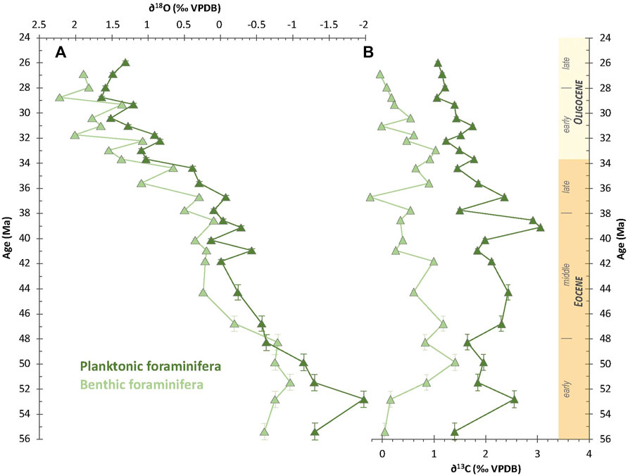
FIGURE 7. Temporal evolution of foraminiferal (A) δ¹⁸O (in ‰ VPDB) and (B) δ¹³C (in ‰ VPDB) for benthic and planktonic species along the studied time interval.

Foraminiferal δ¹³C values are between -0.24 and +1.41‰ and +1.06 to +3.06‰ for benthic and planktonic species respectively (Figure 7B). Benthic and planktonic signals do not show similar temporal trends. For benthic foraminifera, δ¹³C increases from +0.04 to +1.41‰ during the 55.4 to 49.9 Ma interval and progressively decreases down to −0.24‰ at 36.7 Ma. Then it increases up to +1.03‰ at 33.0 Ma before decreasing down to -0.05‰ at 26.9 Ma. For planktonic foraminifera, δ¹³C values range from +1.39‰ to +2.54‰ and do not show major evolution along the 55.4 to 40.1 Ma interval. Then planktonic foraminifera δ¹³C values increase up to +3.05‰ at 39.1 and +2.91‰ at 38.5 Ma before decreasing down to +1.07‰ at 26.0 Ma.

4 Discussion

4.1 Pristine seawater chemical signal

SEM observations of planktonic foraminifera indicate minor recrystallizations as evidenced by “frosty” test texture (Sexton et al., 2006; Hollis et al., 2015; Shepherd et al., 2021) (Figure 3). Nonetheless, for both benthic and planktonic foraminifera, the LREE depletion compared to HREE as well as the marked Ce and La anomalies are typical of pristine seawater chemical signatures (e.g., Elderheld and Greaves, 1982; Elderfield, 1988; Bau and Dulski, 1996; Kamber and Webb, 2001; Bolhar et al., 2004; Deng et al., 2017; Hodel et al., 2021) (Figure 4). These features would undoubtedly have been deleted by early-diagenetic fluids and detrital contamination (e.g., Bolhar et al., 2004; Deng et al., 2017). This is in agreement with the Al/Ca and Sr/Ca ratios presented in Section 3.4.1, showing that diagenetic or recrystallization overprints can be excluded, except for three samples (Figure 5). Very low Al/Ca and Sr/Ca ratios in Al/Ca vs. Mg/Ca and Sr/Ca vs. Mg/Ca diagrams (Figure 5) also discard a significant effect of secondary coatings on Mg/Ca ratios and therefore on Mg/Ca-derived temperatures. Indeed, all the samples that we further use in our discussion are below the calculated threshold values calculated by Hollis et al. (2015) to discard samples with Mg/Ca-temperatures possibly biased by more than 1°C by detrital silicates, early-diagenetic (coatings) and/or recrystallization processes. Hence, even if we did not use the conventional oxidizing-reducing cleaning of Barker et al. (2003), these chemical features attest of the validity of our Mg/Ca-derived temperatures. The latter is ultimately confirmed by the perfect consistency between 1) our Mg/Ca-SFT record and all the δ¹⁸O-SFT records available for Site 277 (Hollis et al., 2012; Pascher et al., 2015; Shepherd et al., 2021; this study; Figure 8), and 2) our Subbotina Sp. Mg/Ca-derived thermocline temperatures and those of Hines et al. (2017) on the same site, whom applied a LA-ICP-MS method specially designed to remove the effects of potential post-depositional diagenetic contamination on Mg/Ca ratios (Figure 8). Therefore, we conclude that the elementary chemistry of the analysed benthic and planktonic foraminifera from Site 277 reflects pristine seawater composition for the investigated elements.

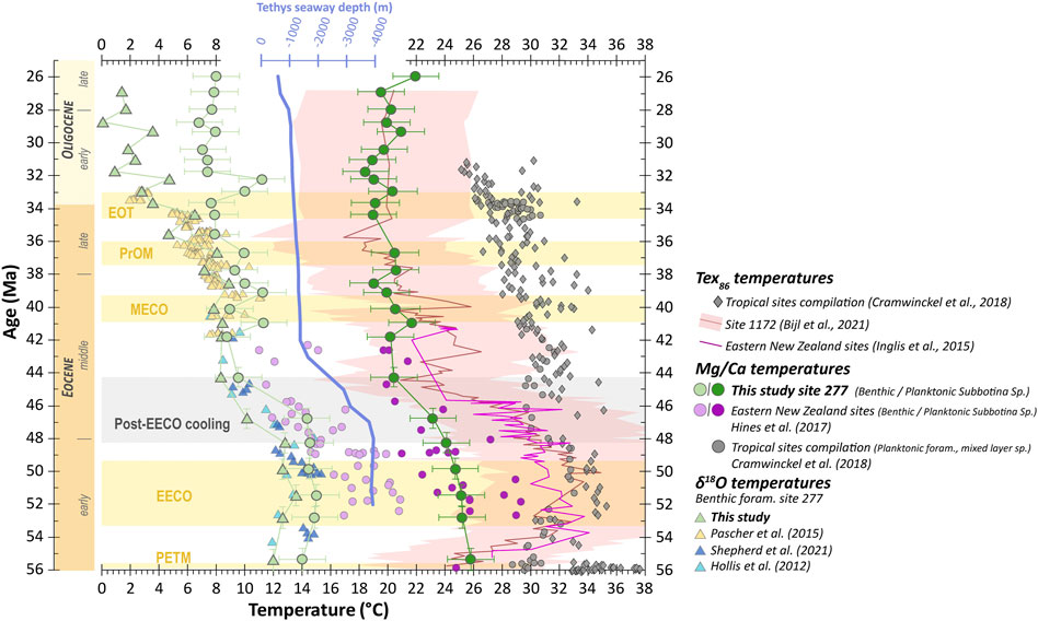
FIGURE 8. Temporal evolution of foraminiferal Mg/Ca- and δ¹⁸O-derived SSTs (here thermocline temperatures obtained on Subbotina sp. foraminifera) and SFTs (seafloor temperatures obtained on Cibicidoides sp. and Gyroidinoides sp.) compared to available data from Hollis et al. (2012), Pascher et al. (2015), Hines et al. (2017), and Shepherd et al. (2021). TEX₈₆-derived SSTs (mixed-layer temperatures) for Site 1172 (Bijl et al., 2021) and Eastern New Zealand sites (Mid-Waipara and Hampden, Inglis et al., 2015) are also represented for comparison. Compilation of Mg/Ca- and TEX₈₆-derived SSTs (mixed-layer temperatures) from tropical sites worldwide by Cramwinckel et al. (2018) is also shown for comparison. It is worth noting that the post-EECO cooling that we and other authors noticed in the southwest Pacific Ocean is not visible in that compilation. Tethys seaway depth evolution is from Straume et al. (2020).

Nevertheless, we cannot exclude potential effects of secondary processes on the O isotope compositions (e.g., Katz et al., 2010; Hollis et al., 2015). Indeed, δ¹⁸O of foraminiferal calcite and derived temperatures are known to be more easily biased by such processes. Post-mortem recrystallization of planktonic tests once deposited on the seafloor can induce a cool bias on δ¹⁸O-derived sea-surface temperatures (SSTs) by partially recording the bottom ocean temperature (Katz et al., 2010; Hollis et al., 2015). This bias is reflected by the relatively close δ¹⁸O values of benthic and planktonic species throughout the studied interval, suggesting a temperature offset of only ∼2°C between bottom and surface waters, much lower than the one estimated from Mg/Ca ratios (∼12°C). For this reason, we focus our study on Mg/Ca-derived SSTs, which appear to be less affected by post-mortem recrystallization (Katz et al., 2010; Hollis et al., 2015) than δ¹⁸O-derived SSTs. Finally, it is worth noting that the planktonic Subbotina sp. foraminifera picked for this study are thought to be thermocline-dwelling species (e.g., Pearson et al., 2006; Hollis et al., 2012; Pascher et al., 2015). Thus, calculated SSTs likely correspond to an integration of the thermocline paleotemperatures.

4.2 Southwest Pacific seawater temperatures

4.2.1 Early Eocene Climate Optimum

With a maximum temperature of 26°C in the early Eocene and a minimum temperature of 18°C in the late Oligocene, our Mg/Ca-derived SSTs are in line with TEX₈₆ temperatures calculated and compiled by Bijl et al. (2009, 2021) for ODP Site 1,172 (Tasmania) located at an equivalent paleolatitude of ∼60°S (see Figure 1 for Site 1172 location) (Figure 8). These high SSTs (from 23 to 26°C in the thermocline) are consistent with the multi-proxy SSTs of 26–28°C calculated by Hollis et al. (2012) for the Early Eocene Climate Optimum (EECO, Figure 1A) in the Canterbury Basin (New Zealand), as well as with numerous geochemical studies indicating warm subtropical-cool tropical conditions in the southwest Pacific Ocean in the early Eocene (Bijl et al., 2009; Hollis et al., 2009, 2015; Liu et al., 2009; Creech et al., 2010; Sluijs et al., 2011; Hines et al., 2017; Crouch et al., 2020) (Figure 8). Despite these numerous studies displaying consistently high temperatures, such high SSTs at high latitude (above 50°S) are still debated. This notably hinges on the fact that “proxy-based paleoclimate reconstructions from the southwest and tropical Pacific imply little to no latitudinal temperature gradient during the early-Eocene, which is difficult to reconcile with the known climate dynamics and model studies” (in Hines et al., 2017, see also Cramwinckel et al., 2018 and Hollis et al., 2019). Recently, Shepherd et al. (2021) indicated that nannofossil assemblages from DSDP sites 207 and 277 (see Figure 1 for sites locations) more likely attest to warm temperate rather than tropical conditions. Several hypotheses have been proposed to explain this thermal overestimation, notably calibration issues, seasonal bias, and physiological processes (Sluijs et al., 2006; Hollis et al., 2012; Taylor et al., 2013; Hollis et al., 2015; Inglis et al., 2015). However, as raised by Hollis et al. (2015), given the consistency between the various proxies used in these studies (δ¹⁸O, Mg/Ca, and TEX₈₆), such overestimation must rely on common factor(s) affecting all proxies like a warm-season bias rather than calibration issues or physiological factors (e.g., Sluijs et al., 2011; Hollis et al., 2012, 2015). Benthic Mg/Ca and δ¹⁸O data also testify to high and stable seafloor temperatures (SFTs) during the early Eocene, ranging from 14 to 15°C and 12–14°C, respectively, between 56 Ma and 48 Ma. These data are also consistent with those from Hollis et al. (2012) and Shepherd et al. (2021) showing similar SFTs for the Canterbury Basin and Site 277 (Figure 8A).

To explain such high seasonal SSTs and high SFTs during the early Eocene, Hines et al. (2017) proposed that an intensification of a proto-East Australian Current (EAC) during the PETM may have resulted in the distribution of tropical temperatures down into the high-latitude southwest Pacific Ocean. Similarly, based on the Nelson and Cooke (2001) study, Shepherd et al. (2021) proposed that New Zealand and the Tasman Sea were likely bathed by warm waters originating from the western limb of the South Pacific anticyclonic gyre and the southward extension of a proto-EAC (Figure 9A).

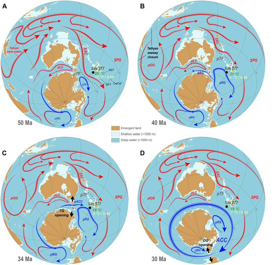
FIGURE 9. Paleogeographic reconstructions illustrating possible paleoceanographic evolutions along the Eocene-Oligocene interval. (A), (B), (C) and (D) correspond to snapshots at 50 Ma, 40 Ma, 34 Ma and 30 Ma, respectively. Paleogeographic and paleobathymetric data are from Straume et al. (2020). Reconstructions were realized using the GPlate software. Arrows represent warmer (red) and cooler (blue) oceanic currents. They result from an attempt of harmonization of several global and regional studies coupled with the results of the present study (this study and Nelson and Cooke, 2001; Huber et al., 2004; Stickley et al., 2004; Bijl et al., 2009; Sijp et al., 2011; Hollis et al., 2012; Pascher et al., 2015; Hines et al., 2017; Houben et al., 2019; Ladant et al., 2020; Straume et al., 2020; Hodel et al., 2021; Shepherd et al., 2021; Sauermilch et al., 2021). The size of the arrows is arbitrary. Abbreviations stand for: pIOG, proto-Indian Ocean Gyre; pLC, proto-Leeuwin Current; pWG, proto-Weddell Gyre; pRG: proto-Ross Gyre; ACC, Antarctic Circumpolar Current; pTF: proto-Tasman Front; EAC, East Australian Current; SPG, South Pacific Gyre, TG, Tasmanian Gateway; DG, Drake Passage Gateway.

4.2.2 Middle Eocene cooling

Following the EECO, our Mg/Ca-derived SSTs show a progressive cooling during the early-mid-Eocene, which intensifies from 48.3 Ma to 44.3 Ma with SSTs decreasing from 24°C down to 20°C (Figure 8A). Synchronously, both Mg/Ca- and δ¹⁸O-derived SFTs also attest to a marked cooling of ca. 4°C following the EECO (Figure 8A). In line with the emergence of cool-water nannofossil taxa at Site 277 from 49 Ma (Shepherd et al., 2021), this cooling likely marks the transition toward temperate conditions in the southwest Pacific Ocean (see also Hollis et al., 2012, 2021).

A first hypothesis to explain this southwest Pacific Ocean cooling could be a global climate event due to decreasing atmospheric pCO₂ (e.g., Zachos et al., 2008). However, other local mechanisms have been proposed given the apparent lack of (sub-) equatorial cooling at that time (e.g., Bijl et al., 2013; Cramwinckel et al., 2018; Shepherd et al., 2021; Figure 8). Indeed, a comparison of SSTs between southwest Pacific and tropical sites shows that all southwest Pacific sites are affected by a significant cooling following the EECO, whereas no comparable drop is observed for tropical sites (Figure 8 and references therein). To explain this, Bijl et al. (2013) proposed that local cooling could have been caused by a westbound flowing current across the Tasmanian Gateway producing a “cooling of Antarctic surface waters and coasts, which was conveyed to global intermediate waters through invigorated deep convection in southern high latitudes.” More recently, Shepherd et al. (2021) proposed that a migration of the proto-Ross gyre and the proto-Tasman front (cooler waters, e.g., Nelson and Cooke, 2001; Huber et al., 2004) toward lower latitudes could also explain this post-EECO cooling.

As previously mentioned, the source of warm waters bathing the Campbell Plateau before this cooling was likely a proto-EAC fed by warm tropical-equatorial waters originating from both the tropical Indian Ocean and a South Pacific anticyclonic gyre (e.g., Nelson and Cooke, 2001; Hines et al., 2017; Shepherd et al., 2021) (Figure 9A). Therefore, we hypothesize that the northward migration proto-Ross gyre proposed by Shepherd et al. (2021) may have resulted from a retreat of this proto-EAC. Indeed, the Tasman gateway was not significantly opened at that time (Stickley et al., 2004) and the proto-EAC was thus likely to be the main control on the northward expansion of the proto-Ross gyre. Based on recent studies, we propose two mechanisms to explain such a proto-EAC weakening:

1) Paleomagnetic studies suggest a rifting between Southern Pacific and Indian oceans between 50 and 40 Ma (e.g., Van Hinsbergen et al., 2015). Meanwhile, these studies (see also Bijl et al., 2021) show a southward drift of the Pacific sector of Antarctica over this time interval, relative to the position of the Earth’s spin axis. This possibly has relocated the proto-EAC, reduced its strength, and leads to an effective northward expansion of the proto-Ross gyre.

2) An alternate hypothesis is linked to the Tethys seaway. In the early Eocene, the Tethys seaway played a key role in global ocean circulation by driving an eastward TCC (Tethys Circum global Current), which provided warm saline water masses to the tropical Indian Ocean (e.g., Jovane et al., 2009; Ladant et al., 2020; Straume et al., 2020). Hamon et al. (2013) also modeled that the “final closure of the eastern Tethys seaway played a major role in the oceanic circulation reorganization during the middle Miocene”, notably by inducing “strong changes in the latitudinal density gradient and ultimately the reinforcement of the Antarctic Circumpolar Current”. This confirms the important influence of the Tethyan inputs on the Southern Ocean paleoceanography. Recently, Straume et al. (2020) suggested that a major step in the Tethys seaway closure occured from 48 Ma to 42 Ma (depth loss of ca. 3,000 m), synchronously with the possible proto-EAC retreat and associated post-EECO cooling (Figure 8). Thus, we hypothesize that this Tethys seaway shoaling from 48 Ma to 42 Ma, possibly coupled with the partial obstruction of the Tethys-tropical Indian Ocean connection by the northward migration of the Indian plate (e.g., Straume et al., 2020), could also have resulted in a significant reduction of the warm eastward tropical-equatorial fluxes feeding the proto-EAC at that time (Figure 9B).

Further studies, notably modeling studies, are needed to validate or invalidate these hypotheses.

4.2.3 Middle to late Eocene

Following the post-EECO cooling, SSTs remained stable from 44 Ma to 26 Ma (20°C on average with a standard deviation of ±1.8°C) (Figure 8), without noticeable shift at the Eocene-Oligocene Transition (33.7 Ma). This trend is consistent with the TEX₈₆-derived SSTs of Bijl et al. (2021). In contrast, SFTs show more fluctuations during this time interval. After 44.3 Ma onward, SFTs calculated from both proxies remain stable until 36.7 Ma except for two isolated temperature rises of ca. +2°C noticeable in the Mg/Ca record at 41.0 Ma and 39.1 Ma. Then both proxies record a SFT drop of more than 3°C for δ¹⁸O data and ca. 2°C for Mg/Ca data between 36.7 Ma and 35.6 Ma. Our sampling resolution is not sufficient to study in detail these potential short-lived events, which are not the purpose of this study.

4.2.4 Eocene-Oligocene transition: Major cooling, massive ice cap build-up, or both?

At the time of the EOT glaciation (from 34.4 Ma to 33.0 Ma), δ¹⁸O-derived SFTs drop from 6°C to 3°C. Then δ¹⁸O-derived SFTs progressively decrease during the Oligocene (with two positive peaks at 32.2 Ma and 29.3 Ma) down to a SFT of 1.37°C at 26.9 Ma. Interestingly, Mg/Ca-derived SFTs and SSTs do not follow this cooling trend and remain rather stable from 35.6 Ma to 26.0 Ma (Figure 8).

A possible explanation is that local phenomena could have influenced seawater temperature at Site 277 across the EOT. Indeed, this absence of cooling at the EOT in our Mg/Ca record is also noticeable in the TEX₈₆ record of Bijl et al. (2021) from ODP Site 1172 (Figure 8). This could be due to a throughflow of the warm proto-Leeuwin current at the same time as EOT cooling as suggested by Houben et al. (2019) and/or to a subtropical front developing at these sites as the Tasmanian gateway opens (Sauermilch et al., 2021).

However, the dichotomy between ice-independent (Mg/Ca and TEX₈₆) and ice-dependent (δ¹⁸O) records remains puzzling. As mentioned above, southwest Pacific Mg/Ca and TEX₈₆-derived temperatures remain constant across the EOT, but δ¹⁸O-derived temperatures drop (Figure 8). Several other sites show the same ambiguity worldwide: for instance, DSDP Site 511 at the Falkland Plateau (Houben et al., 2019), ODP sites 689 and 748 at Maud Rise and the Kerguelen Plateau (Bohaty et al., 2012). Lear et al. (2004) even suggest warming of ca. 2°C in the deep South Atlantic (DSDP Site 522) and Equatorial Pacific (ODP Site 1,218) oceans following the EOT. Therefore, either Mg/Ca and TEX₈₆ temperatures are biased similarly or δ¹⁸O temperatures are biased.

Based on the fact that the foraminiferal δ¹⁸O is ice-dependent while the Mg/Ca is not, authors firstly concluded that this apparent absence of cooling in the benthic foraminifera Mg/Ca record implied that most of the δ¹⁸O increase was due to an ice volume increase, modifying the seawater δ¹⁸O, rather than a major cooling (e.g., Lear et al., 2000; Billups and Schrag, 2003). Then, it has been shown that these results imply ice volume that cannot be accommodated by Antarctica alone (e.g., Coxall et al., 2005; DeConto et al., 2008) and therefore suggest a massive Arctic ice-cap formation. Based on a compilation of U₃₇^k' and TEX₈₆-derived SSTs at low and high latitudes, Liu et al. (2009) proposed that the EOT was accompanied by a heterogeneous cooling and modeled “that Northern Hemisphere glaciation was not required to accommodate the magnitude of continental ice growth during this time”. Today the timing of the Northern Hemisphere ice-cap onset is a subject of controversy (see Hutchinson et al., 2021 for a review). Several studies have found evidence of massive Arctic ice-cap formation (at least ephemeral) as early as the Eocene (e.g., Tripati et al., 2005, 2008; Moran et al., 2006; Eldrett et al., 2007; Stickley et al., 2009; Darby, 2014; Bernard et al., 2016; Tripati and Darby, 2018) while others argue for a Miocene (e.g., DeConto et al., 2008) or even a Pliocene (e.g., Zachos et al., 2001) Arctic glaciation. Given this controversy, several authors looked for alternative hypotheses to explain the lack of foraminiferal Mg/Ca-derived temperature cooling following the EOT. These hypotheses are the following:

1) Based on the sensitivity of benthic foraminiferal Mg/Ca to seawater saturation state (Dekens et al., 2002; Elderfield et al., 2006; Rosenthal et al., 2006; Yu and Elderfield, 2008), it has been proposed that the benthic foraminifera Mg/Ca signal might have been affected by an increase in bottom seawater saturation state associated with a deepening of the calcite compensation depth (CCD) (Lear et al., 2004, 2008, 2010; Coxall et al., 2005; Pusz et al., 2011; Bohaty et al., 2012).

2) Another possibility is that other forcings may have modified the Mg and Ca distribution in seawater and thus modified the Mg/Ca_seawater ratio itself (e.g., Bohaty et al., 2012). If so, our temperature calculation from foraminiferal Mg/Ca using a unique Mg/Ca seawater value for the whole Eocene-Oligocene (Mg/Ca_sw^t=t = 1.6 mol.mol⁻¹ in Eq. 1, Hollis et al., 2015; Hines et al., 2017) is biased.

However, several observations call these hypotheses into question. Indeed, a possible role of carbonate saturation state change (CCD deepening) at Site 277 is improbable given: 1) its shallow depth (i.e. 1000-1500 m, well above the lysocline at lower to middle bathyal water depths since the Paleocene, Hollis et al., 1997): and 2) the Mg/Ca temperature data show that neither SFT nor SST cooled. Concerning a sudden Mg/Ca_seawater ratio change, our calculations of Mg/Ca-derived temperatures considering an unrealistic switch from an Eocene Mg/Ca_seawater ratio (1.6 mol.mol⁻¹, Hollis et al., 2015; Hines et al., 2017) to a modern Mg/Ca_seawater ratio (5.17 mol.mol⁻¹, Stanley and Hardie, 1998; Evans and Müller, 2012) at the EOT does not result in a good agreement between Mg/Ca and δ¹⁸O temperatures (see Supplementary Figure S1). Finally, as previously mentioned, the TEX₈₆-derived temperatures of Bijl et al. (2021) at Site 1172, which are not dependent on seawater carbonate nor to Mg chemistry, are also constant across the EOT (see Figure 8).

Hence, these findings tend to confirm that the δ¹⁸O record has been affected by something other than seawater cooling across the EOT (e.g., Cramer et al., 2011). This is probably an important ice control supported by Antarctica alone (e.g. Zachos et al., 2001; DeConto et al., 2008; Liu et al., 2009), or possibly by a bipolar glaciation as suggested by recent studies (Darby, 2014; Bernard et al., 2016; Tripati and Darby, 2018). We do not have the key to resolve this enigma. However, we believe that it constitutes a critical obstacle in the understanding of this major climate transition and that further studies are needed. In particular, the depicted changes in seawater temperatures obtained from foraminiferal δ¹⁸O values will remain biased as long as the evolution of the ice-volume component present in the δ¹⁸O fractionation equation (see Eq. 2) is not further constrained.

4.3 Redox state of the southwest Pacific Ocean

The negative Ce anomaly (Ce/Ce* < 1) is a common chemical feature of present-day seawater (e.g., Elderheld and Greaves, 1982; Elderfield, 1988; Grenier et al., 2013; Hathorne et al., 2014; Deng et al., 2017). This relies on the two valence states of Ce (III and IV) while other REE (apart Eu) are only trivalent. In modern oxic seawater, the oxidation of Ce³⁺ ions to Ce⁴⁺ ions leads to the precipitation of CeO₂, hence removing Ce from seawater leading to a negative Ce anomaly in the REE pattern. Logically, the more oxygenated the seawater is, the more Ce is removed and the stronger the negative Ce anomaly is. Therefore, the amplitude of the Ce anomaly, quantified by the Ce/Ce* ratio, constitutes a powerful proxy to reconstruct the past seawater redox state (e.g., Bau and Dulski, 1996; Deng et al., 2017). Because foraminifera accurately record the REE chemistry of the seawater in which they thrive in their calcitic test, the temporal evolution of the Ce/Ce* values in well-preserved foraminifera allows to finely document the past seawater redox state (e.g., Kamber et al., 2014; Osborne et al., 2017; Remmelzwaal et al., 2019; Hodel et al., 2021). At Site 277, Ce/Ce* values are similar for benthic and planktonic foraminifera throughout the studied interval. This is due to the fact that REE are at least partly incorporated in authigenic Fe-Mn coatings once on the seafloor and therefore benthic and planktonic foraminifera both record bottom water REE composition (e.g., Roberts et al., 2010; Molina-Kescher et al., 2014; Osborne et al., 2017).

4.3.1 Weakly oxygenated ocean along the early to middle Eocene at site 277

In the early to middle Eocene, Ce/Ce* values are variable but remain high (Ce/Ce*>0.67) until 41.8 Ma (Figure 10), which indicates hypoxic bottom water conditions at the Campbell Plateau at that time (e.g., Remmelzwaal et al., 2019). Since this hypoxia is associated with very high SFTs and SSTs (above 8°C and 22°C, respectively, Figure 8), we propose that these low-oxygen conditions could be related to this particular warm climate. Indeed, previous studies of oceans’ redox state evolution argued that the main warming events of the Earth’s history were often accompanied by open ocean hypoxic and shelf domain anoxic/euxinic episodes (e.g., Monteiro et al., 2012; Pälike et al., 2014; Chang et al., 2018; Remmelzwaal et al., 2019; Cornaggia et al., 2020; Clarkson et al., 2021). Among them, the PETM (ca. 56 Ma) and the ETM2 (ca. 54 Ma) are the last hyperthermal events for which widespread ocean deoxygenation has been proposed (e.g., Dickson and Cohen, 2012; Pälike et al., 2014; Chang et al., 2018; Yao et al., 2018; Remmelzwaal et al., 2019; Harper et al., 2020; Clarkson et al., 2021). Recently, Remmelzwaal et al. (2019) showed that temperature was likely the main driver of ocean deoxygenation during the PETM. Here, with similar temperatures (Figure 8), we suggest that the warm climate of the early to middle Eocene could have resulted in a poorly oxygenated ocean too. If so, the Campbell Plateau could have been particularly impacted by ocean deoxygenation given its rather shallow (ca. 1,000–1,500 mbsl) and isolated setting (e.g., Hollis et al., 1997).

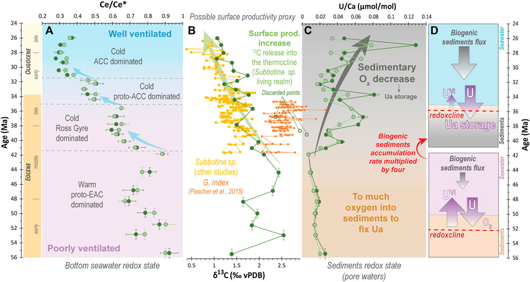
FIGURE 10. Evolution of bottom water redox state, primary productivity, and sediments redox state along the studied time interval. (A) Evolution of the foraminiferal Ce anomaly reflecting bottom water conditions. (B) δ¹³C data of thermocline dwelling Subbotina sp., a possible proxy for surface productivity. Three samples have been discarded because of probable contamination or picking error. We notably suspect accidental picking of surface mixed-layer species instead of Subbotina sp. for these samples given the fact that they fall in the Globigerinatheka index (G. index) composition field in Pascher et al. (2015) data. Compiled data for Subbotina sp. δ¹³C values for Site 277 are from Keigwin (1980), Murphy and Kennett, 1986, and Pascher et al. (2015). (C) Evolution of foraminiferal U/Ca ratios in Site 277 foraminifera. (D) Scheme of the redoxcline shoaling (allowing U fixation on foraminifera tests) in response to an increase of productivity export denoted by Subbotina sp. δ¹³C data and drastic increase of the sedimentation rate from 42–40 Ma at Site 277.

From 41.8 Ma onwards, the Ce/Ce* values decrease to ca. 0.6 and stabilize between 40.1 Ma and 35.6 Ma. This indicates progressive seawater oxygenation that further stabilized (Figure 10A). This possibly constitutes a response to the cooling of the surface and bottom waters between 48.3 and 44.3 Ma at Site 277 (retreat of the warm proto-EAC) and enhanced ventilation (vertical mixing through upwelling) at Site 277 once a proto-Ross gyre dominated system was established (Figure 8, Figure 9A,B, Figure 10A).

4.3.2 Enhanced ventilation after the Tasmanian and Drake Passage gateways opening

After the first oxygenation step, foraminiferal Ce/Ce* values drop a second time between 35.6 Ma and 34.4 Ma (Figure 4B, Figure 10A) indicating a further oxygenation enhancement of the Campbell Plateau bottom waters. This drop is synchronous with the deep opening of the Tasmanian gateway from 35.5 Ma by Stickley et al. (2004). Finally, a last drop of the foraminiferal Ce/Ce* values occurs between 31.8 Ma and 31.0 Ma. This third oxygenation step led to well-oxygenated bottom waters at the Campbell Plateau during the late Oligocene (Ce/Ce* < 0.4) (Figure 9D, Figure 10A). Interestingly, as for the previous step, this ventilation enhancement is synchronous with a major gateway opening, namely the Drake Passage gateway, which likely opened to deep flow from ca. 31 Ma allowing the ACC onset (e.g., Scher et al., 2015; Hodel et al., 2021 and references therein). Hence, these results 1) tend to validate the timing of the Tasman and Drake Passage gateways deep openings ca. 35 Ma and ca. 31 Ma, respectively, and 2) testify that the opening of these gateways had major consequences on the Southern Ocean ventilation and water masses redox state Hodel et al. (2021) (Figure 9). Further work is needed with a higher spatial and temporal resolution to better constrain the involved mechanisms. In particular, it would be interesting to measure the evolution of the foraminiferal Ce anomaly for several other drill sites in the southwest Pacific and southern Indian Ocean and compare it to that of Site 277 that we provide in this study.

4.4 Paleoproductivity and sedimentary redox state

Based on the fact that the U/Ca in cultured planktonic foraminifera decreases with increasing seawater [CO₃²⁻], the foraminiferal U/Ca ratio has been first considered as a promising proxy for seawater carbonate chemistry (e.g., Russell et al., 1996, 2004; Katz et al., 2010; Keul et al., 2013). However, Boiteau et al. (2012) pointed out that the U contents in downcore foraminifera were often much higher than the U incorporation threshold into biogenic calcite (lattice-bound U/Ca < 15 nmol.mol⁻¹). As a result, these authors suggested that most of the U measured in downcore foraminifera was hosted by reduced sedimentary coating (U⁴⁺ fixation, while U⁶⁺ remains soluble in oxygenated environments). From that point, they proposed that the foraminiferal U/Ca ratio was directly related to authigenic U in sedimentary piles, providing “a simple means of evaluating redox changes in sediments where bulk sediment U data is unavailable or unreliable” (in Boiteau et al., 2012). Also, Boiteau et al. (2012), and later Chen et al. (2017), identified a clear correlation between glacial cycles and foraminiferal U/Ca in sediments of the last 400 kyrs, mirrored by high U/Ca ratios during glacial maxima and low U/Ca ratios during interglacial. They attributed this obvious correlation to either a “shoaling of the oxygen penetration depth (i.e. sedimentary redoxcline) due to increased export production or to reduced bottom water oxygen concentrations” (Boiteau et al., 2012). These processes both result in reducing conditions favoring authigenic U precipitation or adsorption onto the foraminifera tests during glacial intervals. Chase et al. (2001) also identified such glacial-interglacial U/Ca variations in foraminifera from a well-ventilated Sub-Antarctic setting during the last glacial maximum. Therefore, they argued that this tendency (high U/Ca ratios during glacial maxima and low U/Ca ratios during interglacials) more likely results from increased glacial productivity in the Sub-Antarctic region rather than from bottom water redox change.

Similarly, the temporal trends of the foraminiferal Ce anomaly, which recorded bottom seawater redox changes, attest to enhanced ventilation of the water masses at Site 277 from 41.8 Ma onwards (Figure 10A). Thus, the increase in foraminiferal U/Ca that we observe is unlikely to be related to a lower bottom seawater oxygenation and more likely relies on productivity/sedimentary processes (e.g., Chase et al., 2001; Boiteau et al., 2012). Thus, we hypothesize that a productivity enhancement and export may have reduced the oxygen penetration depth into the sediment, promoting more reductive conditions conducive to U fixation on foraminifera tests (e.g., Chase et al., 2001; Boiteau et al., 2012) (Figure 10D). This hypothesis is strengthened by 1) the sedimentation rate evolution, which is multiplied by four from 41.8 Ma without a major change in biogenic vs detrital contributions (the sedimentation remained mainly biogenic, Kennett et al., 1975; Hollis et al., 1997) (Figure 2) and 2) the Subbotina sp. δ¹³C values, which start decreasing from that time (Figure 10B). Indeed, metabolic processes preferentially incorporate ¹²C, thus phytoplankton blooms deplete the shallowest surface seawater in ¹²C and enrich deeper surface water (where Subbotina sp. live) in ¹²C after organic matter mineralization (e.g., Katz et al., 2010). Therefore, even if δ¹³C is not only a productivity proxy and has to be interpreted carefully, Subbotina sp. δ¹³C evolves as we would expect if there was a major phytoplanktonic bloom. This strengthens the idea of enhanced primary productivity from 42 Ma. If so, the rather shallow depth of Site 277, which remained well above the lysocline along the Eocene-Oligocene interval, is compatible with the fact that the organic matter did not have time to fully mineralize during its sinking through the water column, therefore allowing its deposition and burial. Then, the decomposition of this remaining organic matter into the sediment likely promoted reducing conditions and a shoaling of the sedimentary redoxcline, allowing the fixation of U on both benthic and planktonic foraminifera tests at Site 277 (Figure 10D). Increasing productivity has been already noticed in the Southern Ocean during the Eocene-Oligocene in response to seawater cooling and circulation intensification (e.g., Diester-Haass and Zahn, 1996; Plancq et al., 2014). Similarly, we can reasonably hypothesize that at Site 277, cooler seawater and more vigorous ocean circulation may have promoted an enhanced vertical mixing and nutrient supply through upwelling (Diester-Haass and Zahn, 1996; Miller et al., 2009; Plancq et al., 2014) once a proto-Ross gyre dominated system was established from ca. 42 Ma, then following the Tasmanian Gateway opening from ca. 35 Ma and finally with the establishment of the ACC following the Drake Passage Gateway opening from ca. 31 Ma.

5 Conclusion

Our integrated geochemical study of Site 277 foraminifera brings new insights into the paleoceanographic evolution of the southwest Pacific during the major climate transition of the Eocene-Oligocene.

Both Mg/Ca- and δ¹⁸O-derived temperatures attest to very high SSTs (from ca. 24°C–26°C in the thermocline) and SFTs (from ca. 12°C to 14°C) at Site 277 during the EECO (from 55.4 Ma to 48.1 Ma). Such high temperatures are in line with other studies relating subtropical conditions in this area. This indicates that despite its high latitude location, the Campbell Plateau was bathed by warm waters, possibly originating from a proto-EAC fed by warm tropical-equatorial waters originating from both a South Pacific anticyclonic gyre and the tropical Indian Ocean (Figure 9A). Weak foraminiferal Ce anomaly (Ce/Ce* values close to 1) along this warm early to middle Eocene (from 55.4 Ma to 41.8 Ma) attests to poorly oxygenated bottom seawater at Site 277 at that time. Between 48.3 and 44.3 Ma, both Mg/Ca and δ¹⁸O data recorded a marked bottom and surface cooling of ca. 4°C. Given the absence of an equivalent cooling at higher latitudes, we hypothesize that a proto-EAC weakening and a Ross-gyre enhancement pushed the proto-Tasman front (cooler waters) towards lower latitudes (Figure 9B). Then, bottom and surface temperatures remained rather constant until the EOT. Interestingly, our benthic Mg/Ca- and δ¹⁸O-signals are significantly different from the EOT: δ¹⁸O-temperatures decrease while Mg/Ca-temperatures remain constant. This dichotomy suggests that the hypothesis of a dominant ice control on the global EOT δ¹⁸O decrease has to be reconsidered.

Major changes in redox and paleoproductivity took place from 41.8 Ma onwards, i.e., with the onset of a proto-Ross gyre dominated system (Figure 9B). We notably identified a major increase in productivity export from that time, which likely promoted more reductive sedimentary conditions. From 41.8 Ma as well, a drop of foraminiferal Ce/Ce* values attests to enhanced ventilation of bottom waters after the establishment of a proto-Ross gyre dominated system. Ce/Ce* values then drop a second time between 35.6 Ma and 34.4 Ma and a third time between 31.8 Ma and 31.0 Ma, synchronously with the Tasmanian and Drake Passage gateways opening. These results tend to confirm the timing of these major gateways opening and attest that their opening had major consequences on the Southern Ocean ventilation and water masses’ redox state.

Thereby, altogether these results shed light on the role that major oceanic gateway closings and openings play on the Earth’s climate by driving ocean currents and associated heat fluxes, water masses redox state and primary productivity fluxes.

Data availability statement

The original contributions presented in the study are included in the article/Supplementary Material, further inquiries can be directed to the corresponding author.

Funding

FH thanks IODP France for his postdoc fellowship and post cruise supports. This research used samples and data provided by the International Ocean Discovery Program (IODP). IODP is sponsored by the United States National Science Foundation (NSF) and participating countries under management of the Joint Oceanographic Institution (JOI) Inc.

Acknowledgments

Authors acknowledge two reviewers and M. Sprovieri for their suggestions to improve this manuscript. R. Guilbaud and R. Tostevin are thanked for their advices and discussions about sedimentary redox state and U/Ca ratio evolutions. Authors acknowledge the LEGOS clean lab team for sharing their lab, A. Marquet on the ICP-MS and L. Emmanuel for O and C isotope analyses.

Conflict of interest

The authors declare that the research was conducted in the absence of any commercial or financial relationships that could be construed as a potential conflict of interest.

Publisher’s note

All claims expressed in this article are solely those of the authors and do not necessarily represent those of their affiliated organizations, or those of the publisher, the editors and the reviewers. Any product that may be evaluated in this article, or claim that may be made by its manufacturer, is not guaranteed or endorsed by the publisher.

Supplementary material

The Supplementary Material for this article can be found online at: https://www.frontiersin.org/articles/10.3389/feart.2022.998237/full#supplementary-material

References

Anand, P., Elderfield, H., and Conte, M. H. (2003). Calibration of Mg/Ca thermometry in planktonic foraminifera from a sediment trap time series. Paleoceanography 18, 2. doi:10.1029/2002PA000846
Barth, M. G., McDonough, W. F., and Rudnick, R. L. (2000). Tracking the budget of Nb and Ta in the continental crust. Chem. Geol. 165, 197–213. doi:10.1016/S0009-2541(99)00173-4
Bau, M., and Dulski, P. (1996). Distribution of yttrium and rare-Earth elements in the penge and kuruman iron-formations, transvaal super-group, South Africa. Precambrian Res. 79 (1–2), 37–55. doi:10.1016/0301-9268(95)00087-9
Bernard, T., Steer, P., Gallagher, K., Szulc, A., Whitham, A., and Johnson, C. (2016). Evidence for Eocene–Oligocene glaciation in the landscape of the east Greenland margin. Geology 44, 895–898. doi:10.1130/G38248.1
Bijl, P., Frieling, J., Cramwinckel, M., Boschman, C., Sluijs, A., and Peterse, F. (2021). Maastrichtian-rupelian paleoclimates in the southwest Pacific – A critical evaluation of biomarker paleothermometry and dinoflagellate cyst paleoecology at ocean drilling Program site 1172. Clim. Past. Discuss., 1–82. doi:10.5194/cp-2021-18
Bijl, P. K., Bendle, J. A. P., Bohaty, S. M., Pross, J., Schouten, S., Tauxe, L., et al. (2013). Eocene cooling linked to early flow across the Tasmanian Gateway. Proc. Natl. Acad. Sci. U. S. A. 110, 9645–9650. doi:10.1073/pnas.1220872110
Bijl, P. K., Schouten, S., Sluijs, A., Reichart, G. J., Zachos, J. C., and Brinkhuis, H. (2009). Early palaeogene temperature evolution of the southwest Pacific Ocean. Nature 461, 776–779. doi:10.1038/nature08399
Billups, K., and Schrag, D. P. (2003). Application of benthic foraminiferal Mg/Ca ratios to questions of Cenozoic climate change. Earth Planet. Sci. Lett. 209, 181–195. doi:10.1016/S0012-821X(03)00067-0
Bohaty, S. M., Zachos, J. C., and Delaney, M. L. (2012). Foraminiferal Mg/Ca evidence for Southern Ocean cooling across the eocene-oligocene transition. Earth Planet. Sci. Lett. 317–318, 251–261. doi:10.1016/j.epsl.2011.11.037
Boiteau, R., Greaves, M., and Elderfield, H. (2012). Authigenic uranium in foraminiferal coatings: A proxy for ocean redox chemistry. Paleoceanography 27, 3. doi:10.1029/2012PA002335
Bolhar, R., Kamber, B. S., Moorbath, S., Fedo, C. M., and Whitehouse, M. J. (2004). Characterisation of early Archaean chemical sediments by trace element signatures. Earth Planet. Sci. Lett. 222, 43–60. doi:10.1016/j.epsl.2004.02.016
Burgess, C. E., Pearson, P. N., Lear, C. H., Morgans, H. E. G., Handley, L., Pancost, R. D., et al. (2008). Middle Eocene climate cyclicity in the southern Pacific: Implications for global ice volume. Geol. 36, 651–654. doi:10.1130/G24762A.1
Chang, L., Harrison, R. J., Zeng, F., Berndt, T. A., Roberts, A. P., Heslop, D., et al. (2018). Coupled microbial bloom and oxygenation decline recorded by magnetofossils during the Palaeocene–Eocene Thermal Maximum. Nat. Commun. 9, 4007–4009. doi:10.1038/s41467-018-06472-y
Chase, Z., Anderson, R. F., and Fleisher, M. Q. (2001). Evidence from authigenic uranium for increased productivity of the glacial subantarctic ocean. Paleoceanography 16, 468–478. doi:10.1029/2000PA000542
Chen, P., Yu, J., and Jin, Z. (2017). An evaluation of benthic foraminiferal U/Ca and U/Mn proxies for deep ocean carbonate chemistry and redox conditions. Geochem. Geophys. Geosyst. 18, 617–630. doi:10.1002/2016GC006730
Clarkson, M. O., Lenton, T. M., Andersen, M. B., Bagard, M. L., Dickson, A. J., and Vance, D. (2021). Upper limits on the extent of seafloor anoxia during the PETM from uranium isotopes. Nat. Commun. 12, 399. doi:10.1038/s41467-020-20486-5
Cornaggia, F., Bernardini, S., Giorgioni, M., Silva, G. L. X., Nagy, A. I. M., and Jovane, L. (2020). Abyssal oceanic circulation and acidification during the middle eocene climatic optimum (MECO). Sci. Rep. 10, 6674. doi:10.1038/s41598-020-63525-3
Coxall, H. K., Wilson, P. A., Pälike, H., Lear, C. H., and Backman, J. (2005). Rapid stepwise onset of Antarctic glaciation and deeper calcite compensation in the Pacific Ocean. Nature 433, 53–57. doi:10.1038/nature03135
Cramer, B. S., Miller, K. G., Barrett, P. J., and Wright, J. D. (2011). Late Cretaceous-Neogene trends in deep ocean temperature and continental ice volume: Reconciling records of benthic foraminiferal geochemistry (δ18O and Mg/Ca) with sea level history. J. Geophys. Res. 116, C12023. doi:10.1029/2011JC007255
Cramwinckel, M. J., Huber, M., Kocken, I. J., Agnini, C., Bijl, P. K., Bohaty, S. M., et al. (2018). Synchronous tropical and polar temperature evolution in the Eocene. Nature 559, 382–386. doi:10.1038/s41586-018-0272-2
Creech, J. B., Baker, J. A., Hollis, C. J., Morgans, H. E. G., and Smith, E. G., C. (2010). Eocene sea temperatures for the mid-latitude southwest Pacific from Mg/Ca ratios in planktonic and benthic foraminifera. Earth Planet. Sci. Lett. 299, 483–495. doi:10.1016/j.epsl.2010.09.039
Crouch, E. M., Shepherd, C. L., Morgans, H. E. G., Naafs, B. D. A., Dallanave, E., Phillips, A., et al. (2020). Climatic and environmental changes across the early Eocene climatic optimum at mid-Waipara River, Canterbury Basin, New Zealand. Earth. Sci. Rev. 200, 102961. doi:10.1016/j.earscirev.2019.102961
Darby, D. A. (2014). Ephemeral formation of perennial sea ice in the Arctic Ocean during the middle Eocene. Nat. Geosci. 7, 210–213. doi:10.1038/ngeo2068
DeConto, R. M., and Pollard, D. (2003). Rapid Cenozoic glaciation of Antarctica induced by declining atmospheric CO2. Nature 421, 245–249. doi:10.1038/nature01290
DeConto, R. M., Pollard, D., Wilson, P. A., Pälike, H., Lear, C. H., and Pagani, M. (2008). Thresholds for Cenozoic bipolar glaciation. Nature 455, 652–656. doi:10.1038/nature07337
Dekens, P. S., Lea, D. W., Pak, D. K., and Spero, H. J. (2002). Core top calibration of Mg/Ca in tropical foraminifera: Refining paleotemperature estimation. Geochem. Geophys. Geosyst. 3, 1–29. doi:10.1029/2001GC000200
Deng, Y., Ren, J., Guo, Q., Cao, J., Wang, H., and Liu, C. (2017). Rare Earth element geochemistry characteristics of seawater and porewater from deep sea in Western Pacific. Sci. Rep. 7, 16539. doi:10.1038/s41598-017-16379-1
Dickson, A. J., and Cohen, A. S. (2012). A molybdenum isotope record of Eocene Thermal Maximum 2: Implications for global ocean redox during the early Eocene. Paleoceanography 27. doi:10.1029/2012PA002346
Diester-Haass, L., and Zahn, R. (1996). Eocene-Oligocene transition in the Southern Ocean: History of water mass circulation and biological productivity. Geol. 24 (2), 163–166. doi:10.1130/0091-7613(1996)024<0163:eotits>2.3.co;2
Elderfield, H. (1988). The oceanic chemistry of the rare-Earth elements. Phil. Trans. Roy. Sot. Lond. A 325, 105–106.
Elderfield, H., Yu, J., Anand, P., Kiefer, T., and Nyland, B. (2006). Calibrations for benthic foraminiferal Mg/Ca paleothermometry and the carbonate ion hypothesis. Earth Planet. Sci. Lett. 250, 633–649. doi:10.1016/j.epsl.2006.07.041
Elderheld, H., and Greaves, M. J. (1982). The rare Earth elements in seawater. Nature 296, 214–219. doi:10.1038/296214a0
Eldrett, J., Harding, I., Wilson, P., Butler, E., and Roberts, A. P. (2007). Continental ice in Greenland during the Eocene and Oligocene. Nature 446, 176–179. doi:10.1038/nature05591
Elsworth, G., Galbraith, E., Halverson, G., and Yang, S. (2017). Enhanced weathering and CO2 drawdown caused by latest Eocene strengthening of the Atlantic meridional overturning circulation. Nat. Geosci. 10, 213–216. doi:10.1038/ngeo2888
Evans, D., and Müller, W. (2012). Deep time foraminifera Mg/Ca paleothermometry: Nonlinear correction for secular change in seawater Mg/Ca. Paleoceanography 27. doi:10.1029/2012PA002315
Goldner, A., Herold, N., and Huber, M. (2014). Antarctic glaciation caused ocean circulation changes at the Eocene–Oligocene transition. Nature 511, 574–577. doi:10.1038/nature13597
Gradstein, F. M. (2020). “Introduction,” in Geologic time scale 2020 (Elsevier), 3–20. doi:10.1016/b978-0-12-824360-2.00001-2
F. M. Gradstein, J. G. Ogg, M. D. Schmitz, and G. M. Ogg (Editors). (2012). The geologic time scale 2012 (Elsevier).
Grenier, M., Jeandel, C., Lacan, F., Vance, D., Venchiarutti, C., Cros, A., et al. (2013). From the subtropics to the central equatorial Pacific Ocean: Neodymium isotopic composition and rare Earth element concentration variations. J. Geophys. Res. Oceans 118, 592–618. doi:10.1029/2012JC008239
Hamon, N., Sepulchre, P., Lefebvre, V., and Ramstein, G. (2013). The role of eastern tethys seaway closure in the middle Miocene climatic transition (ca. 14 Ma). Clim. Past. 9, 2687–2702. doi:10.5194/cp-9-2687-2013
Harper, D. T., Hönisch, B., Zeebe, R. E., Shaffer, G., Haynes, L. L., Thomas, E., et al. (2020). The magnitude of surface ocean acidification and carbon release during eocene thermal maximum 2 (ETM-2) and the paleocene-eocene thermal maximum (PETM). Paleoceanogr. Paleoclimatol. 35, e2019PA003699. doi:10.1029/2019PA003699
Hathorne, E. C., Stichel, T., Brück, B., and Frank, M. (2014). Rare Earth element distribution in the Atlantic sector of the Southern Ocean: The balance between particle scavenging and vertical supply. Mar. Chem. 177, 157–171. doi:10.1016/j.marchem.2015.03.011
Henehan, M. J., Edgar, K. M., Foster, G. L., Penman, D. E., Hull, P. M., Greenop, R., et al. (2020). Revisiting the middle eocene climatic optimum “carbon cycle conundrum” with new estimates of atmospheric pCO2 from boron isotopes. Paleoceanogr. Paleoclimatol. 35, e2019PA003713. doi:10.1029/2019PA003713
Hines, B. R., Hollis, C. J., Atkins, C. B., Baker, J. A., Morgans, H. E. G., and Strong, P. C. (2017). Reduction of oceanic temperature gradients in the early Eocene southwest Pacific Ocean. Palaeogeogr. Palaeoclimatol. Palaeoecol. 475, 41–54. doi:10.1016/j.palaeo.2017.02.037
Hodel, F., Grespan, R., de Rafélis, M., Dera, G., Lezin, C., Nardin, E., et al. (2021). Drake Passage gateway opening and Antarctic Circumpolar Current onset 31 Ma ago: The message of foraminifera and reconsideration of the Neodymium isotope record. Chem. Geol. 570, 120171. doi:10.1016/j.chemgeo.2021.120171
Hollis, C. J., Dunkley Jones, T., Anagnostou, E., Bijl, P. K., Cramwinckel, M. J., Cui, Y., et al. (2019). The DeepMIP contribution to PMIP4: Methodologies for selection, compilation and analysis of latest Paleocene and early Eocene climate proxy data, incorporating version 0.1 of the DeepMIP database. Geosci. Model. Dev. 12 (7), 3149–3206. doi:10.5194/gmd-12-3149-2019
Hollis, C. J., Handley, L., Crouch, E. M., Morgans, H. E. G., Baker, J. A., Creech, J., et al. (2009). Tropical sea temperatures in the high-latitude south pacific during the eocene. Geology 37, 99–102. doi:10.1130/G25200A.1
Hollis, C. J., Hines, B. R., Littler, K., Villasante-Marcos, V., Kulhanek, D. K., Strong, C. P., et al. (2015). The paleocene-eocene thermal maximum at DSDP site 277, Campbell Plateau, southern Pacific ocean. Clim. Past. 11, 1009–1025. doi:10.5194/cp-11-1009-2015
Hollis, C. J., Tayler, M. J. S., Andrew, B., Taylor, K. W., Lurcock, P., Bijl, P. K., et al. (2014). Organic-rich sedimentation in the south Pacific ocean associated with late Paleocene climatic cooling. Earth. Sci. Rev. 134, 81–97. doi:10.1016/j.earscirev.2014.03.006
Hollis, C. J., Taylor, K. W. R., Handley, L., Pancost, R. D., Huber, M., Creech, J. B., et al. (2012). Early Paleogene temperature history of the southwest Pacific Ocean: Reconciling proxies and models. Earth Planet. Sci. Lett. 349350, 53–66. doi:10.1016/j.epsl.2012.06.024–
Hollis, C. J., Waghorn, D. B., Strong, C. P., and Crouch, E. M. (1997). Integrated Paleogene biostratigraphy of DSDP site 277 (Leg 29): foraminifera, calcareous nannofossils, Radiolaria, and palynomorphs, 97/9. Lower Hutt: Institute of Geological & Nuclear Sciences science reportInstitute of Geological & Nuclear Sciences, 1–73.
Houben, A. J. P., Bijl, P. K., Sluijs, A., Schouten, S., and Brinkhuis, H. (2019). Late eocene Southern Ocean cooling and invigoration of circulation preconditioned Antarctica for full-scale glaciation. Geochem. Geophys. Geosyst. 20, 2019GC008182–2234. doi:10.1029/2019GC008182
Huber, M., Brinkhuis, H., Stickley, C. E., Döös, K., Sluijs, A., Warnaar, J., et al. (2004). Eocene circulation of the Southern Ocean: Was Antarctica kept warm by subtropical waters? Paleoceanography 19. doi:10.1029/2004PA001014
Hutchinson, D. K., Coxall, H. K., Lunt, D. J., Steinthorsdottir, M., De Boer, A. M., Baatsen, M., et al. (2021). The eocene-oligocene transition: A review of marine and terrestrial proxy data, models and model-data comparisons. Clim. Past. 17, 269–315. doi:10.5194/cp-17-269-2021
Inglis, G. N., Farnsworth, A., Lunt, D., Foster, G. L., Hollis, C. J., Pagani, M., et al. (2015). Descent toward the Icehouse: Eocene sea surface cooling inferred from GDGT distributions. Paleoceanography 30, 1000–1020. doi:10.1002/2014PA002723
Jeandel, C., Delattre, H., Grenier, M., Pradoux, C., and Lacan, F. (2013). Rare Earth element concentrations and Nd isotopes in the Southeast Pacific Ocean. Geochem. Geophys. Geosyst. 14, 328–341. doi:10.1029/2012GC004309
Jovane, L., Coccioni, R., Marsili, A., and Acton, G. (2009). “The late Eocene greenhouse-icehouse transition: Observations from the Massignano global stratotype section and point (GSSP),” in The late Eocene earth—hothouse, icehouse, and Impacts (Geological Society of America), 149–168. doi:10.1130/2009.245210
Kamber, B. S., Greig, A., and Collerson, K. D. (2005). A new estimate for the composition of weathered young upper continental crust from alluvial sediments, Queensland, Australia. Geochim. Cosmochim. Acta 69, 1041–1058. doi:10.1016/j.gca.2004.08.020
Kamber, B. S., Webb, G. E., and Gallagher, M. (2014). The rare Earth element signal in Archaean microbial carbonate: Information on ocean redox and biogenicity. J. Geol. Soc. Lond. 171, 745–763. doi:10.1144/jgs2013-110
Kamber, B. S., and Webb, G. E. (2001). The geochemistry of late Archaean microbial carbonate: Implications for ocean chemistry and continental erosion history. Geochimica Cosmochimica Acta 65 (152), 2509–2525. doi:10.1016/S0016-7037(01)00613-5
Katz, M. E., Cramer, B. S., Franzese, A., Hönisch, B., Miller, K. G., Rosenthal, Y., et al. (2010). Traditional and emerging geochemical proxies in foraminifera. J. Foraminifer. Res. 40, 165–192. doi:10.2113/gsjfr.40.2.165
Katz, M. E., Katz, D. R., Wright, J. D., Miller, K. G., Pak, D. K., Shackleton, N. J., et al. (2003). Early Cenozoic benthic foraminiferal isotopes: Species reliability and interspecies correction factors. Paleoceanography 18. doi:10.1029/2002PA000798
Keigwin, L. D. (1980). Palaeoceanographic change in the pacific at the eocene–oligocene boundary. Nature 287, 722–725. doi:10.1038/287722a0
Kennedy-Asser, A. T., Lunt, D. J., Valdes, P. J., Ladant, J.-B., Frieling, J., and Lauretano, V. (2020). Changes in the high-latitude southern hemisphere through the eocene–oligocene transition: A model–data comparison. Clim. Past. 16, 555–573. doi:10.5194/cp-16-555-2020
Kennett, J. P. (1977). Cenozoic evolution of Antarctic glaciation, the circum-Antarctic Ocean, and their impact on global paleoceanography. J. Geophys. Res. 82, 3843–3860. doi:10.1029/JC082i027p03843
Kennett, J. P., Houtz, R. E., Andrews, P. B., Edwards, A. R., Gostin, V. A., Hajós, M., et al. (1975). Initial Reports of the Deep Sea Drilling Project, 29. U.S. Government Printing Office. Initial Reports of the Deep Sea Drilling Project. doi:10.2973/dsdp.proc.29.1975
Kennett, J. P., and Exon, N. F. (2004). Paleoceanographic evolution of the Tasmanian Seaway and its climatic implications. American Geophysical Union AGU, 345–367. doi:10.1029/151GM19
Keul, N., Langer, G., Nooijer, L. J., Nehrke, G., Reichart, G., and Bijma, J. (2013). Incorporation of uranium in benthic foraminiferal calcite reflects seawater carbonate ion concentration. Geochem. Geophys. Geosyst. 14, 102–111. doi:10.1029/2012GC004330
Killick, R., and Eckley, I. (2014). Changepoint: An R package for changepoint Analysis. J. Stat. Softw. 58, 1–19. doi:10.18637/jss.v058.i03
Kim, S. T., and O’Neil, J. R. (1997). Equilibrium and nonequilibrium oxygen isotope effects in synthetic carbonates. Geochim. Cosmochim. Acta 61, 3461–3475. doi:10.1016/S0016-7037(97)00169-5
Ladant, J.-B., Donnadieu, Y., Lefebvre, V., and Dumas, C. (2014). The respective role of atmospheric carbon dioxide and orbital parameters on ice sheet evolution at the Eocene-Oligocene transition. Paleoceanography 29, 810–823. doi:10.1002/2013PA002593
Ladant, J. B., Poulsen, C. J., Fluteau, F., Tabor, C. R., Macleod, K. G., Martin, E. E., et al. (2020). Paleogeographic controls on the evolution of Late Cretaceous ocean circulation. Clim. Past. 16, 973–1006. doi:10.5194/cp-16-973-2020
Lear, C. H., Bailey, T. R., Pearson, P. N., Coxall, H. K., and Rosenthal, Y. (2008). Cooling and ice growth across the Eocene-Oligocene transition. Geol. 36, 251–254. doi:10.1130/G24584A.1
Lear, C. H., Elderfield, H., and Wilson, P. A. (2000). Cenozoic deep-sea temperatures and global ice volumes from Mg/Ca in benthic foraminiferal calcite. Science 287, 269–272. doi:10.1126/science.287.5451.269
Lear, C. H., Mawbey, E. M., and Rosenthal, Y. (2010). Cenozoic benthic foraminiferal Mg/Ca and Li/Ca records: Toward unlocking temperatures and saturation states. Paleoceanography 25. doi:10.1029/2009PA001880
Lear, C. H., Rosenthal, Y., Coxall, H. K., and Wilson, P. A. (2004). Late Eocene to early Miocene ice sheet dynamics and the global carbon cycle. Paleoceanography 19, 1–11. doi:10.1029/2004PA001039
Lear, C. H., Rosenthal, Y., and Slowey, N. (2002). Benthic foraminiferal Mg/Ca-paleothermometry: A revised core-top calibration. Geochim. Cosmochim. Acta 66, 3375–3387. doi:10.1016/S0016-7037(02)00941-9
Liu, Z., Pagani, M., Zinniker, D., DeConto, R., Huber, M., Brinkhuis, H., et al. (2009). Global cooling during the eocene-oligocene climate transition. Science 323, 1187–1190. doi:10.1126/science.1166368
Miller, K. G., Wright, J. D., Katz, M. E., Wade, B., Browning, J. V., Cramer, B. S., et al. (2009). “Climate threshold at the eocene-oligocene transition: Antarctic ice sheet influence on Ocean circulation,”. Editors C. Koeberl, and A. Montanari Geological Society of America, China, Vol. 452, 169–178.late Eocene Earth – hothouse, icehouse, impacts.
Molina-Kescher, Mario, Frank, Martin, and Hathorne, Ed C. (2014). South Pacific dissolved Nd isotope compositions and rare Earth element distributions: Water mass mixing versus biogeochemical cycling. Geochimica Cosmochimica Acta 127, 171–189. doi:10.1016/j.gca.2013.11.038
Monteiro, F. M., Pancost, R. D., Ridgwell, A., and Donnadieu, Y. (2012). Nutrients as the dominant control on the spread of anoxia and euxinia across the Cenomanian-Turonian oceanic anoxic event (OAE2): Model-data comparison. Paleoceanography 27. doi:10.1029/2012PA002351
Moran, K., Backman, J., Brinkhuis, H., Clemens, S. C., Cronin, T., Dickens, G. R., et al. (2006). The cenozoic palaeoenvironment of the arctic ocean. Nature 441, 601–605. doi:10.1038/nature04800
Müller, R. D., Cannon, J., Qin, X., Watson, R. J., Gurnis, M., Williams, S., et al. (2018). GPlates: Building a virtual earth through deep time. Geochem. Geophys. Geosyst. 19 (7), 2243–2261. doi:10.1029/2018gc007584
Murphy, M. G., and Kennett, J. P. (1986). Initial reports DSDP, Leg 90, noumea, New Caledonia to wellington, New Zealand. Part 2 1347–1360. doi:10.2973/dsdp.proc.90.140.1986Development of latitudinal thermal gradients during the oligocene: Oxygen-isotope evidence from the southwest pacific
Nelson, C. S., and Cooke, P. J. (2001). History of oceanic front development in the New Zealand sector of the Southern Ocean during the Cenozoic - a synthesis. N. Z. J. Geol. Geophys. 44, 535–553. doi:10.1080/00288306.2001.9514954
Osborne, A. H., Hathorne, E. C., Schijf, J., Plancherel, Y., Böning, P., and Frank, M. (2017). The potential of sedimentary foraminiferal rare Earth element patterns to trace water masses in the past. Geochem. Geophys. Geosyst. 18, 1550–1568. doi:10.1002/2016GC006782
Pagani, M., Huber, M., Liu, Z., Bohaty, S. M., Henderiks, J., Sijp, W., et al. (2011). The role of carbon dioxide during the onset of Antarctic glaciation. Science 334, 1261–1264. doi:10.1126/science.1203909
Pälike, C., Delaney, M. L., and Zachos, J. C. (2014). Deep-sea redox across the Paleocene-Eocene thermal maximum. Geochem. Geophys. Geosyst. 15, 1038–1053. doi:10.1002/2013GC005074
Pascher, K. M., Hollis, C. J., Bohaty, S. M., Cortese, G., McKay, R. M., Seebeck, H., et al. (2015). Expansion and diversification of high-latitude radiolarian assemblages in the late Eocene linked to a cooling event in the southwest Pacific. Clim. Past. 11, 1599–1620. doi:10.5194/cp-11-1599-2015
P. N. Pearson, R. K. Olsson, B. T. Huber, C. Hemleben, and W. A. Berggren (Editors) (2006). Atlas of Eocene planktonic foraminifera.
Plancq, J., Mattioli, E., Pittet, B., Simon, L., and Grossi, V. (2014). Productivity and sea-surface temperature changes recorded during the late Eocene–early Oligocene at DSDP Site 511 (South Atlantic). Palaeogeogr. Palaeoclimatol. Palaeoecol. 407, 34–44. doi:10.1016/j.palaeo.2014.04.016
Pusz, A. E., Thunell, R. C., and Miller, K. G. (2011). Deep water temperature, carbonate ion, and ice volume changes across the Eocene-Oligocene climate transition. Paleoceanography 26. doi:10.1029/2010PA001950
R Development Core Team. (2019). R: A language and environment for statistical computing. Vienna, Austria: R Foundation for Statistical Computing.
Rae, J. W. B., Foster, G. L., Schmidt, D. N., and Elliott, T. (2011). Boron isotopes and B/Ca in benthic foraminifera: Proxies for the deep ocean carbonate system. Earth Planet. Sci. Lett. 302, 403–413. doi:10.1016/j.epsl.2010.12.034
Remmelzwaal, S. R. C., Dixon, S., Parkinson, I. J., Schmidt, D. N., Monteiro, F. M., Sexton, P., et al. (2019). Investigating ocean deoxygenation during the PETM through the Cr isotopic signature of foraminifera. Paleoceanogr. Paleoclimatol. 34, 917–929. doi:10.1029/2018PA003372
Roberts, N. L., Piotrowski, A. M., McManus, J. F., and Keigwin, L. D. (2010). Synchronous deglacial overturning and water mass source changes. Science 327, 75–78. doi:10.1126/science.1178068
Rosenthal, Y., Lear, C. H., Oppo, D. W., and Linsley, B. K. (2006). Temperature and carbonate ion effects on Mg/Ca and Sr/Ca ratios in benthic foraminifera: Aragonitic species Hoeglundina elegans. Paleoceanography 21. doi:10.1029/2005PA001158
Russell, A. D., Emerson, S., Mix, A. C., and Peterson, L. C. (1996). The use of foraminiferal uranium/calcium ratios as an indicator of changes in seawater uranium content. Paleoceanography 11, 649–663. doi:10.1029/96PA02058
Russell, A. D., Hönisch, B., Spero, H. J., and Lea, D. W. (2004). Effects of seawater carbonate ion concentration and temperature on shell U, Mg, and Sr in cultured planktonic foraminifera. Geochim. Cosmochim. Acta 68, 4347–4361. doi:10.1016/j.gca.2004.03.013
Sauermilch, I., Whittaker, J. M., Klocker, A., Munday, D. R., Hochmuth, K., Bijl, P. K., et al. (2021). Gateway-driven weakening of ocean gyres leads to Southern Ocean cooling. Nat. Commun. 12, 6465–6468. doi:10.1038/s41467-021-26658-1
Sauermilch, I., Whittaker, J. M., Klocker, A., Munday, D. R., Hochmuth, K., LaCasce, J. H., et al. (2019). Tectonic gateway driven cooling of Antarctica with high resolution ocean models. Vienna: American Geophysical Union, Fall Meeting 2019, PP11B–02.
Scher, H. D., Bohaty, S. M., Smith, B. W., and Munn, G. H. (2014). Isotopic interrogation of a suspected late Eocene glaciation. Paleoceanography 29, 628–644. doi:10.1002/2014PA002648
Scher, H. D., Whittaker, J. M., Williams, S. E., Latimer, J. C., Kordesch, W. E. C., and Delaney, M. L. (2015). Onset of antarctic circumpolar current 30 million years ago as tasmanian gateway aligned with westerlies. Nature 523, 580–583. doi:10.1038/nature14598
Sexton, P. F., Wilson, P. A., and Pearson, P. N. (2006). Microstructural and geochemical perspectives on planktic foraminiferal preservation: “Glassy” versus “frosty. Geochem. Geophys. Geosyst. 7 (12). doi:10.1029/2006GC001291
Shepherd, C. L., Kulhanek, D. K., Hollis, C. J., Morgans, H. E. G., Strong, C. P., Pascher, K. M., et al. (2021). Calcareous nannoplankton response to early Eocene warmth, southwest Pacific Ocean. Mar. Micropaleontol. 165, 101992. doi:10.1016/j.marmicro.2021.101992
Sijp, W. P., England, M. H., and Huber, M. (2011). Effect of the deepening of the Tasman Gateway on the global ocean. Paleoceanography 26, 2011PA002143. doi:10.1029/2011PA002143
Sluijs, A., Bijl, P. K., Schouten, S., Röhl, U., Reichart, G. J., and Brinkhuis, H. (2011). Southern Ocean warming, sea level and hydrological change during the Paleocene-Eocene thermal maximum. Clim. Past. 7, 47–61. doi:10.5194/cp-7-47-2011
Sluijs, A., Schouten, S., Pagani, M., Woltering, M., Brinkhuis, H., Damsté, J. S. S., et al. (2006). Subtropical arctic ocean temperatures during the palaeocene/eocene thermal maximum. Nature 441, 610–613. doi:10.1038/nature04668
Stanley, S. M., and Hardie, L. A. (1998). Secular oscillations in the carbonate mineralogy of reef-building and sediment-producing organisms driven by tectonically forced shifts in seawater chemistry. Palaeogeogr. Palaeoclimatol. Palaeoecol. 144, 3–19. doi:10.1016/S0031-0182(98)00109-6
Stickley, C. E., Brinkhuis, H., Schellenberg, S. A., Sluijs, A., Röhl, U., Fuller, M., et al. (2004). Timing and nature of the deepening of the tasmanian gateway. Paleoceanography 19, doi:10.1029/2004PA001022
Stickley, C. E., St John, K., Koç, N., Jordan, R. W., Passchier, S., Pearce, R. B., et al. (2009). Evidence for middle Eocene Arctic sea ice from diatoms and ice-rafted debris. Nature 460, 376–379. doi:10.1038/nature08163
Straume, E. O., Gaina, C., Medvedev, S., and Nisancioglu, K. H. (2020). Global cenozoic paleobathymetry with a focus on the northern hemisphere oceanic gateways. Gondwana Res. 86, 126–143. doi:10.1016/j.gr.2020.05.011
Taylor, K. W. R., Huber, M., Hollis, C. J., Hernandez-Sanchez, M. T., and Pancost, R. D. (2013). Re-evaluating modern and Palaeogene GDGT distributions: Implications for SST reconstructions. Glob. Planet. Change 108, 158–174. doi:10.1016/j.gloplacha.2013.06.011
Toumoulin, A., Donnadieu, Y., Ladant, J. -B., Batenburg, S. J., Poblete, F., and Dupont-Nivet, G. (2020). Quantifying the effect of the Drake passage opening on the eocene ocean. Paleoceanogr. Paleoclimatol. 35, e2020PA003889. doi:10.1029/2020PA003889
Tripati, A., Backman, J., Elderfield, H., and Ferretti, P. (2005). Eocene bipolar glaciation associated with global carbon cycle changes. Nature 436, 341–346. doi:10.1038/nature03874
Tripati, A., and Darby, D. (2018). Evidence for ephemeral middle Eocene to early Oligocene Greenland glacial ice and pan-Arctic sea ice. Nat. Commun. 9, 1038. doi:10.1038/s41467-018-03180-5
Tripati, A. K., Eagle, R. A., Morton, A., Dowdeswell, J. A., Atkinson, K. L., Bahé, Y., et al. (2008). Evidence for glaciation in the northern hemisphere back to 44 Ma from ice-rafted debris in the Greenland sea. Earth Planet. Sci. Lett. 265, 112–122. doi:10.1016/j.epsl.2007.09.045
Van Hinsbergen, D. J. J., de Groot, L. V., van Schaik, S. J., Spakman, W., Bijl, P. K., Sluijs, A., et al. (2015). A paleolatitude calculator for paleoclimate studies. PLoS One 10, e0126946. doi:10.1371/journal.pone.0126946
Vito, M., and Muggeo, R. (2003). Estimating regression models with unknown break-points. Stat. Med. 22, 3055–3071. doi:10.1002/sim.1545
Yao, W., Paytan, A., and Wortmann, U. G. (2018). Large-scale ocean deoxygenation during the Paleocene-Eocene thermal maximum. Sci. (80-.) 361, 804–806. doi:10.1126/science.aar8658
Yeghicheyan, D., Carignan, J., Valladon, M., Bouhnik Le Coz, M., Samuel, J., Bakkar, M., et al. (2003). Congres Geoanal, 146.The new carbonate reference material CAL-S: Preliminary results
Yu, J., and Elderfield, H. (2008). Mg/Ca in the benthic foraminifera Cibicidoides wuellerstorfi and Cibicidoides mundulus: Temperature versus carbonate ion saturation. Earth Planet. Sci. Lett. 276, 129–139. doi:10.1016/j.epsl.2008.09.015
Zachos, J. C., Dickens, G. R., and Zeebe, R. E. (2008). An early Cenozoic perspective on greenhouse warming and carbon-cycle dynamics. Nature 451, 279–283. doi:10.1038/nature06588
Zachos, J. C., Stott, L. D., and Lohmann, K. C. (1994). Evolution of early cenozoic marine temperatures. Paleoceanography 9, 353–387. doi:10.1029/93PA03266
Zachos, J., Pagani, M., Sloan, L., Thomas, E., and Billups, K. (2001). Trends, rhythms, and aberrations in global climate 65 Ma to present. Science 292, 686–693. doi:10.1126/science.1059412
Keywords: paleoceanography, climate, foraminifera, Eocene, Oligocene, southwest Pacific Ocean
Citation: Hodel F, Fériot C, Dera G, De Rafélis M, Lezin C, Nardin E, Rouby D, Aretz M, Antonio P, Buatier M, Steinmann M, Lacan F, Jeandel C and Chavagnac V (2022) Eocene-Oligocene southwest Pacific Ocean paleoceanography new insights from foraminifera chemistry (DSDP site 277, Campbell Plateau). Front. Earth Sci. 10:998237. doi: 10.3389/feart.2022.998237
Received: 19 July 2022; Accepted: 31 October 2022;
Published: 17 November 2022.
Edited by:
Mario Sprovieri, Institute for the Study of Anthropogenic Impacts and Sustainability in Marine Environment, Department of Earth System Sciences and Technologies for the Environment (CNR), ItalyReviewed by:
Luigi Jovane, University of São Paulo, BrazilHelen C. Bostock, The University of Queensland, Australia
Copyright © 2022 Hodel, Fériot, Dera, De Rafélis, Lezin, Nardin, Rouby, Aretz, Antonio, Buatier, Steinmann, Lacan, Jeandel and Chavagnac. This is an open-access article distributed under the terms of the Creative Commons Attribution License (CC BY). The use, distribution or reproduction in other forums is permitted, provided the original author(s) and the copyright owner(s) are credited and that the original publication in this journal is cited, in accordance with accepted academic practice. No use, distribution or reproduction is permitted which does not comply with these terms.
*Correspondence: F. Hodel, florent.hodel.geo@gmail.com