Seasonal Evolution of Supraglacial Lakes on Baltoro Glacier From 2016 to 2020

1 Introduction

Glaciers with an extensive debris cover respond in a more complex way to changes in climate than those that are debris-free. The glacier response depends on debris thickness and its spatial distribution (Benn et al., 2012). A thin debris cover of only a few centimeters leads to enhanced ablation compared to clean ice due to increased absorption of solar radiation (Ostrem, 1959; Nicholson and Benn, 2006). A debris cover with greater thickness has an insulating effect on the energy transfer to the glacier ice from atmospheric energy sources and reduces ice ablation. With respect to mass balance calculations, various properties of debris cover need to be considered, such as thickness, slope, aspect, and lithology (Mihalcea et al., 2008). Mass balance models can include such debris-dependent surface properties, but due to a lack of empirical data, it is difficult to readily include their impact on glacier melt rates. The ablation of debris-covered glaciers is very heterogeneous with minimal lowering beneath thick debris near the terminus and maximal downwasting in the upper ablation zone near the equilibrium line where thin debris dominates (Benn et al., 2017). Additionally, ice cliffs may contribute up to 25% to ice ablation despite their small area share of 7–8% (Brun et al., 2018; Buri et al., 2021) and supraglacial lakes can be heated by incoming solar radiation and thus can be responsible for considerable subaqueous melting. Previous studies have indicated that lakes could be responsible for 1/8 of total ice loss in the Langtang Valley, Nepal (Miles et al., 2018; Miles et al., 2020).

Only a handful of studies focused on modeling the response of debris-covered glaciers to climatic changes have included a heterogeneous debris thickness distribution in their approach. These studies have found that supraglacial debris delays glacier response to warming and leads to surface lowering and ice cliff backwasting rather than frontal recession (Rowan et al., 2015; Thompson et al., 2016; Brun et al., 2018). Both the surface debris flux and the relationship between debris thickness and the sub-debris melt rate appear to positively affect the glacier length (Anderson and Anderson, 2019), and if a uniform debris thickness value is used rather than one that is spatially variable, the sub-debris ablation rate can be underestimated by 11–30% (Nicholson et al., 2018). The positive interaction between debris thickness, surface ponding, and ice ablation is therefore complex and non-linear and influences glacier dynamics, geometry, and surface properties (Huo et al., 2021). With an up-glacier expansion of the debris cover, these effects will be intensified with time (Mölg et al., 2020; Xie et al., 2020).

Supraglacial lakes mainly form on debris-covered glaciers with a surface inclination of $\le 2^{\text{o}}$ (Reynolds, 2006) and surface velocities of ≤10 m per year. Most of the lakes develop towards the terminus, which is characterized by the lowest surface velocities (Quincey et al., 2007; Sakai, 2012; Kraaijenbrink et al., 2016; Miles K. E. et al., 2017). They form as rain or meltwater accumulates in depressions of the debris cover in early spring. In late summer, many of the lakes drain, while some lakes persist. If the water is able to drain to the glacier bed, it can support basal sliding and hence higher glacier velocities (Sakai and Fujita, 2006; Sakai, 2012; Watson et al., 2016; Benn et al., 2017; Miles E. S. et al., 2017; Miles et al., 2020). Higher precipitation tends to intensify both lake filling and drainage. Stronger spring precipitation leads to increased filling of supraglacial lakes, while stronger winter precipitation causes higher glacier velocities leading to crevasse development and therefore increased pathways for the drainage of lake water (Wendleder et al., 2018). Additionally, warmer springs lead to greater lake drainage later in the same year as more meltwater causes redevelopment of the subsurface drainage system (Liu et al., 2015).

Previous multi-temporal studies mapped the supraglacial lakes in Tian Shan and Himalaya based on optical data. Liu et al. (2015) used an object-based image analysis (OBIA) on Landsat imagery for the months of August and September from 1990 to 2011 to analyze the distribution and seasonal variability of lakes in the Khan Tengri-Tumor Mountains, Tian Shan. Watson et al. (2016) also implemented an OBIA to examine the spatiotemporal dynamics of 9,340 supraglacial ponds located on nine glaciers in the Everest region of Nepal for the period 2000 to 2015. Miles K. E. et al. (2017) combined the Normalized Difference Water Index (NDWI) with two further band ratios to Landsat 5 and 7 imagery on the Langtang Valley, Nepal, to study lake dynamics from 1999 to 2013. Miles et al. (2018) also applied the NDWI, additionally using Otsu’s method to semi-automatically establish an appropriate classification threshold, applied to a dense time series of PlanetScope and RapidEye imagery. An optimized NDWI was introduced by Watson et al. (2018) to account for under- and overestimation of lake areas when using coarser-resolution imagery, using Himalayan debris-covered glaciers with Pleiades, Sentinel-2, and Landsat data to show a proof of concept.

However, to better understand the seasonal evolution of supraglacial lakes and the relationship between lake growth and climate, a continuous time series covering a period of several years is essential. In this study, we combine optical and Synthetic Aperture Radar (SAR) data in order to create such a dense temporal coverage of glacial lake evolution. As SAR signals are able to penetrate clouds, they provide relevant information during the rainy seasons and especially during the period of lake onset. Previous studies have tended to use only optical data and hence have been unable to monitor lake dynamics during the cloudy and rainy seasons. Our multi-sensor approach combining optical and SAR data is a novelty in this application area and could bridge this gap.

We present a semi-automatic approach based on a random forest classifier for the monitoring of supraglacial lake evolution. We apply it to the Baltoro Glacier, located in Karakoram, Pakistan, for the years 2016–2020. The approach uses a multi-temporal and multi-sensor summertime series comprising optical data from Sentinel-2 with a regular acquisition of 5 days and PlanetScope with a very high temporal resolution of 3–5 days and SAR data from Sentinel-1 and TerraSAR-X, both with a regular acquisition of 12 and 11 days, respectively. For the sake of simplicity, we implemented the random forest classifier for all four sensors but with different classification classes and training data. Our aim was to answer the following research questions: 1) What are the characteristic filling and the drainage periods? 2) In what way does the lake area change over the years? 3) What does the spatial lake distribution look like? 4) How does the seasonal evolution vary over the years?

2 Study Site

For our study of glacial lake dynamics, we selected the Baltoro Glacier in the eastern Karakoram. In 2012, the Karakoram region had a glacierized area of 18,000 km² (Collier et al., 2015; Bolch et al., 2012), and approximately 18–22% of it was covered with supraglacial debris (Collier et al., 2015; Scherler et al., 2011; Hewitt, 2011). The Baltoro Glacier is situated in the northern part of Pakistan near the border to India and China (Figure 1). In 2016 the glacier had a total length of 63 km and together with its tributaries covered an area of approximately 524 km² (Mayer et al., 2006). The two major tributaries are the Godwin Austin Glacier and the Baltoro South Glacier, which join at Concordia (4,600 m a.s.l.) to form the main glacier. This main trunk flows in the east-west direction and terminates at 3,410 m a.s.l. The surface velocities derived from SAR data from 1992 to 2017 ranged from 180 to 240 m per year (summer) and 100–140 m per year (winter) between Concordia and Urdukas and decreased to 10–40 m per year near the terminus (Wendleder et al., 2018). Approximately 38% of the Baltoro Glacier is debris-covered, which exceeds the average debris coverage in the Karakoram (Scherler et al., 2011). At Concordia, the debris cover is thin (5–15 cm), increasing in thickness at Urdukas (30–40 cm) and reaching a maximum at the terminus of about 1 m (Mayer et al., 2006; Quincey et al., 2009). Debris-covered glaciers are characterized by the presence of ice sails (Mayer et al., 2006; Evatt et al., 2017), ice cliffs, and supraglacial lakes. On the Baltoro Glacier, ice sails are found in a region from about 6 km downstream to 2 km upstream of Gore (Figure 1) and ice cliffs predominate between the terminus and Gore. Supraglacial lakes are located from the terminus up to Concordia. The majority of those lakes are supraglacial lakes located on the main glacier. There are also two ice-dammed lakes located south of the main trunk, namely, Liligo and Yermanendu Lakes.

FIGURE 1. Overview of Baltoro Glacier, Pakistan, with the glacier boundaries (blue) and the sectors (red) used for the supraglacial lake area analyzed in Sections 4.2 and 4.3. Important place names are indicated. The background image is a Sentinel-2 RGB (B2, B3, B4) composite acquired on July 22, 2019. The glacier boundaries are derived from a Landsat-7 scene acquired on July 12, 2010, based on the Normalized Difference Snow index and manual editing.

The Karakoram climate is characterized by cold winters and mild summers and is dominated by three different systems: 1) the winter westerly disturbances with dominant snowfall in winter and spring, contributing up to two-thirds of the yearly snowfall at high altitudes (Dobreva et al., 2017), 2) the Indian summer monsoon incursion that can lead to higher precipitation, temperatures, and cloud coverage during summer, contributing to snow accumulation in the higher reaches of the glacier (Bookhagen and Burbank, 2006; Thayyen and Gergan, 2010), and 3) the predominantly stable Tibetan Anticyclone that, in the case of an irregular weakening, provokes an incursion of the Indian summer monsoon with large amounts of precipitation (Dobreva et al., 2017). The mean annual precipitation is approximately 1,600 mm per year at 5,300 m a.s.l. (Godwin Austen region) and at 5,500 m a.s.l. (Baltoro South region). As the mean daytime temperature during summer is close to the freezing point at 5,400 m a.s.l., most of the precipitation deposits as snow above this elevation (Mayer et al., 2006).

3 Methodology

3.1 Data

We used a multi-sensor time series with an acquisition every two to four days based on optical data from PlanetScope and Sentinel-2 and SAR data from Sentinel-1 and TerraSAR-X. The sensor characteristics and acquisition parameters are summarized in Table 1 and the data availability is visualized in Figure 2. All four sensor systems are characterized by frequent and consistent coverage. Sentinel-2 has a repeat orbit of 5 days (Gatti and Bertolini, 2013) and provides a continuous and stable time series with relevant information about glacier surface cover like debris, ice, snow, and lakes. The time series is complemented by the high temporal sampling of PlanetScope data. The PlanetScope satellite constellation of about 130 small satellites called “Doves” gathers information every two to five days during cloud-free periods (Miles K. E. et al., 2017; PlanetScope, 2020). The SAR data of Sentinel-1 (Vincent et al., 2019) and TerraSAR-X (Eineder and Fritz, 2009) bridge the gaps of the optical data, which are brought about by cloud cover during the westerly disturbances in April and the monsoon season from the end of May until the end of July. We used data acquired between April and September for the years 2016–2020, and the number and timing of images differed for each season of study, depending on data availability (Table 1).

TABLE 1. Overview of the sensor characteristics and acquisition parameters. In the case of Sentinel-2, only the used spectral bands are listed. The pass directions of the SAR sensors are abbreviated as A for ascending and D for descending. Eineder and Fritz (2009), Vincent et al. (2019), PlanetScope (2020), Gatti and Bertolini (2013).

FIGURE 2. Data availability for the summertime series from 2016 to 2020 with respect to Sentinel-2 (S2), PlanetScope (PS), Sentinel-1 (S1), and TerraSAR-X (TSX). “A” and “D” in parentheses denote the passing direction, i.e., ascending or descending.

For the semi-automated classification, the data needed to be atmospherically corrected, radiometrically calibrated, and orthorectified. Therefore, the Sentinel-2 Multi-Spectral Instrument (MSI) orthorectified Level-1C Top-Of-Atmospheric products were atmospherically corrected to L2A products using MAJA (MACCS ATCOR Joint Algorithm, release 4.2). MAJA is a processor for cloud detection and atmospheric correction and is specifically designed to process optical time series (Hagolle et al., 2017). The PlanetScope Analytic Ortho Scene Products (Level 3B) were already downloaded as orthorectified and atmospherically corrected Surface Reflectance (SR) data. Sentinel-1 Interferometric Wide Swath C-band and TerraSAR-X ScanSAR X-band data were processed to normalized radar backscatter Analysis Ready Data (ARD) using the Multi-SAR System (Schmitt et al., 2015; Schmitt et al., 2020). For the orthorectification, the 3-arcsecond Copernicus-DEM (GLO-90) (Airbus, 2020) was used as it had the best geometric correspondence to Sentinel-2 and PlanetScope data.

The relationship between supraglacial lake evolution and meteorological conditions was analyzed using the corresponding monthly averaged air temperature at 2 m above the surface and total precipitation data of the climate reanalysis dataset ERA5-Land (Hersbach and Bell, 2020). The data are available on a 0.1° by 0.1° grid and were downloaded from the Copernicus Climate Change Service (C3S) Climate Data Store (CDS) (Muñoz-Sabater, 2019).

3.2 Random Forest Classification

We used a random forest approach in classification mode (Breiman, 2001) and applied it to Sentinel-2, PlanetScope, Sentinel-1, and TerraSAR-X images separately in order to detect the supraglacial lakes. Random forest is a common and robust machine learning classification algorithm. It combines the results of many different random decision trees taking the majority votes for each decision tree. Due to the different spectral resolution and the radiometric calibration of Sentinel-2 and PlanetScope, the random forests differed in the number of classes, feature spaces, and training data (Table 2). Training and validation datasets (80:20 ratio) were manually created. Classification and subsequent processing steps were implemented in the open-source software RStudio.

TABLE 2. Overview of the used classes, features, and training data for the random forest classifier. NDI stands for normalized difference index, GLCM for gray level co-occurrence matrix, and ROI for region of interest.

3.2.1 Sentinel-2

For the Sentinel-2 data, we used the same training dataset for all 5 years. The classification results reflect the dominant glacier surface cover types: “dry debris,” “wet debris,” “lakes,” “snow,” and “ice.” As the cloud mask produced by the MAJA algorithm frequently misclassified glacier ice as cloud, we created our own cloud and shadow mask by adding the two classes “shadow” and “clouds.” These masks were generated after the classification in three subsequent steps: 1) since cloud rims were often wrongly classified as water, lake pixels with a distance of 20 m to clouds were deleted; 2) lakes that existed only three to five times in the summertime series were removed (with the exact threshold varying depending on the number of optical data per summertime series); 3) scenes with a cloud coverage over the glacier surface of more than 80% were automatically omitted. For a better distinction of shadows and clouds from lakes, we added the blue and shortwave infrared bands. Shadows showed high absorption in both bands, with lower rates in the shortwave infrared. Clouds showed a high reflection compared to the surrounding area with highest rates in the blue band (Roth, 2019). In order to cover seasonal and annual variations of the water turbidity, the training data were collected in spring and late summer in 2018 and 2019. These 2 years were selected as they had the lowest cloud cover.

3.2.2 PlanetScope

The radiometric quality of PlanetScope data is known to be inconsistent between each of the “Doves” (Houborg and McCabe, 2016; Cooley et al., 2017), which leads to different reflectances between the sensors and prevents the use of a single training dataset as we did for Sentinel-2. For this reason, we chose the random forest approach with individual training data derived from scenes with the same acquisition date. The training data were selected from the classification results of an index approach. Therefore, we introduced the Supraglacial Lake Index (SGLI), a modification of the Normalized Difference Water Index (McFeeters, 1996), specially designed for debris-covered glaciers. The three-step approach is based on two normalized difference indices, one calculated with green and near-infrared and the other with near-infrared and red (Figure 3A). Using this approach, it was possible to discriminate between the classes “debris,” “ice,” and “lake.” For every scene, an individual threshold for the differentiation between the reflectance of “ice” and “lake” was automatically calculated using the unimodal threshold determination (Rosin, 2001). The threshold was defined as the point with the maximum distance between the histogram and line of maximum and minimum peak (Figure 3B). In the final classification, snow was classified as ice because of its spectral similarity, and “shadow” and “cloud” classes were both omitted since all of the PlanetScope imagery we selected was cloud-free. Overall, the random forest yielded an improved classification compared to the index approaches alone, which tend to underestimate the lake area.

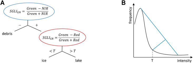
FIGURE 3. (A) Decision tree of the Supraglacial Lake Index (SGLI). “T” stands for threshold derived with the unimodal threshold determination (Rosin, 2001). (B) Method of the unimodal threshold determination (Rosin, 2001). The line between maximum and minimum peak and the maximum distance between histogram and line are displayed in blue.

As the access to PlanetScope data is restricted to a specific download quota per month, only cloud-free data were selected. Therefore, it was not necessary to include the classes “shadow” and “cloud.” Additionally, the data have no shortwave infrared bands, which impedes cloud detection anyway.

3.2.3 Sentinel-1 and TerraSAR-X

The random classifier was executed separately on the ascending and descending orbits of the Sentinel-1 and TerraSAR-X datasets. Due to the similar SAR backscatter of rough debris cover and ice, we could only define the two classes “dry” and “wet.” The discrimination of lake and wet objects is based on the maximal lake extent map of the corresponding year produced by Sentinel-2 data (Miles K. E. et al., 2017). The classification was performed on amplitude and texture information. Therefore, the SAR amplitudes were filtered using a 3 × 3 median filter. The median filter size was a trade-off between the reduction of speckle noise and preserving the supraglacial lake shape (Davies, 2005). Additionally, a gray level co-occurrence matrix (GLCM) texture derived with a 3 × 3 kernel filters in the 0°direction was added to the feature space (Haberäcker, 1987). The use of a single (or combination) of kernel filter(s) in the other three directions (45°, 90°, 135°) had no influence on the classification results.

3.3 Harmonization of SAR-Derived Lake Area

Due to the side-looking radar and the undulating glacier surface, the SAR signal could not map the lake area completely. The SAR-derived lake areas were underestimated and had to be harmonized in order to achieve a consistent lake area time series. The correction was calculated with a linear regression using lake areas derived from optical and SAR data with the same acquisition date. The SAR data were individually corrected depending on their sensor and their pass direction. The linear regression was calculated for each lake separately. In the case of persistent lakes, we used measurements from their complete lifetime rather than just a single year. Pearson’s correlation coefficients before linear regression of all measurements for Sentinel-1 and TerraSAR-X were between 0.89 and 0.93, showing strong evidence of a linear relationship between the two variables. The residual standard error of all linear regressions was between 1,397 m² and 1923 m² and the p-value was between 0.029 and 0.037 (95% confidence level), indicating a significant correlation.

3.4 Multi-Sensor Summertime Series

The classification results of all supraglacial lakes were combined and smoothed to yield a consistent summertime series (de Jonge and van der Loo, 2013). Detected outliers and data gaps were filled with interpolated values. During the harmonization of the lake area, not all SAR-derived areas were corrected due to the absence of any significant associations between the predictor and the outcome variables. The outliers were characterized by their local minimum in the time series and could be detected with the Hausdorff distance (Hausdorff, 1914). This metric is defined as the maximum distance between the original curve and a simplified line between preceding and subsequent measurements. We calculated two simplified lines where the first line is defined by the two previous measurements and the second line by the two following measurements. According to our definition, a negative distance indicated a local minimum. The outlier detection was performed on each lake separately. Missing data were linearly interpolated based on the lake area of the previous and subsequent acquisition. Using the neighboring water level change for interpolation was not possible because each lake had its own characteristic pattern of water level rise and fall, and in addition, cloud coverage often affected large parts of the scene and thus also the neighboring lakes. Based on the summertime series, we analyzed the number of lakes, their total area, the date of maximum area, distribution and duration of water coverage, and the seasonal evolution during the 5 years.

3.5 Seasonal and Trend Components

To examine the seasonal evolution, the time series of the lake area Y_t was analyzed with the multicomponent model following Weatherhead et al. (1998):

where μ is the constant term, S_t is the seasonal component, ω represents the linear trend per year, and N_t is the residual variability. The seasonal component was assumed to be stationary and was modeled as a sinusoid where eight superimposed harmonics are fitted. The uncertainty of the linear trend component was derived as follows:

with σ_r being the standard deviation of the de-trended residuals, n the number of months, and φ the first-order autocorrelation of the residuals.

3.6 Accuracy Assessment of Supraglacial Lake Area

For the accuracy assessment, a reference dataset was manually mapped based on the RGB composite and the NDWI (McFeeters, 1996) calculated with the green and near-infrared band of PlanetScope data. The reference datasets varied in their spatial coverage (Table 4; Supplementary Figure S1) but were consistently selected from 2019, as this year had the lowest cloud coverage and the highest number of coincident pairs between PlanetScope and Sentinel/TerraSAR-X. In order to reflect the accuracy at different turbidity levels and thus the seasonal accuracy, we chose five validation dates for the optical data distributed over the whole summer. Since SAR sensors distinguish only between wet and dry and thus are not sensitive to seasonal turbidity variations, we selected one validation date for each SAR sensor and each pass direction. The PlanetScope data used for the accuracy assessment were omitted in the summertime series. The accuracy was assessed by the comparison of the classified area with the reference area. The classification error was referred to the total area and quantified with the absolute and relative Root Squared Error (RSE) (Liang et al., 2012):

4 Results

4.1 Annual Area Fluctuations

Based on the multi-temporal time series, we calculated the total number and the cumulative area of supraglacial lakes on the main trunk of Baltoro Glacier. We further derived the date of the maximum lake area for each summer season from 2016 to 2020 (Table 3). The cumulative lake area denotes the maximum norm over all lakes during the summer period, whereas the maximum lake area includes all lake areas at a certain point in time. The number of lakes varied from year to year without any clear trend, with a minimum of 379 in 2020 and a maximum of 553 in 2016 (Table 3). The total lake area was lowest in 2017 (3.563 km²) and the highest values in 2018 (5.783 km²). The number and area of lakes larger than 0.01 km² have increased constantly since 2016 with a distinct rise from 2018 onwards. Thus, larger lakes comprised a larger percentage of the total lake area through time. The date of the maximum water level varied between mid-June in 2016 and the end of July in 2017 and 2018. The peak lake area ranged between 1.945 km² in 2017 and 2.587 km² in 2018. Table 3 shows the percentage of ephemeral and permanent lakes at the end of the ablation season. As a reference, we used the classification results from September and October. From 2016 to 2019, the proportion of seasonal lakes was between 54 and 64% and fell to 30 and 33% in 2019 and 2020.

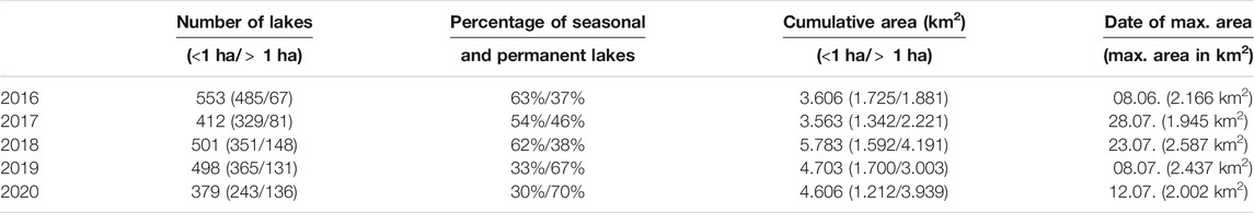
TABLE 3. Number of lakes, cumulative area of lakes in km², percentage of seasonal and permanent lakes at the end of the ablation season, and date and area in km² at maximum lake area for each summer season from 2016 to 2020. The number and cumulative area of lakes are divided into two categories: lakes with an area smaller and larger than 0.01 km².

4.2 Percentage of Lake Area

Figure 4 shows the percentage of lake area compared to total glacier area for each sector (Figure 1 for the definition of the sectors). The lowest lake area was consistently detected above 4,280 m a.s.l. Lake areas were consistently lowest in 2016 and highest in 2018 and 2019. The lowermost sector (3,440–3,710 m a.s.l.) shows the least variation with time, whereas the second sector (3,710–3,880 m a.s.l.) shows the greatest variation, with a total relative area increase of 3.3% between 2017 and 2018. The third (3,880–4,030 m a.s.l.), fourth (4,030–4,160 m a.s.l.), and fifth (4,160–4,280 m a.s.l.) sectors showed an increase of 1.82%, 1.56%, and 2.03%, respectively. However, patterns across the glacier and through time were highly non-linear.

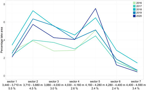
FIGURE 4. Percentage of lake area to the surface area of the main glacier for 2016 to 2020. The glacier was divided into seven sectors from glacier terminus to Concordia Place. Each sector is specified by its altitude range (m a.s.l.) and mean slope (%).

4.3 Size and Altitude Distribution

The number of lakes with altitude (Figure 5) followed a similar distribution to that shown by the percentage of lake area (Figure 4). The sixth and seventh (higher-elevation) sectors consistently had the lowest number of lakes (<50). The second, third, and fourth sectors had the greatest number of lakes, with a maximum number in the second sector (100–120) and a decrease towards the fourth sector (60–90). Lake numbers in the fifth sector varied over the observation period: the highest number was found in 2016 (117) and the lowest number was found in 2017 (60). The years 2018–2020 had between 70 and 90 lakes in this sector. The distribution of the lake area is shown in Figure 5B. The lake area ranged between 500 m² to 440, 000 m². The number of lakes with a size of 1,000–2,000 m² ranged between 15 and 57, whereas those between 2,000 and 3,000 m² varied from 80 to120; otherwise, as the lake size increased, the number of lakes decreased, with the exception of a peak in the size bin of 10,000–20,000 m². The overall number of lakes was less in 2016 and 2017, with maxima in 2018 and 2020 across the glacier surface. There were very few lakes observed in the largest lake classes (20,000–30,000 m²).

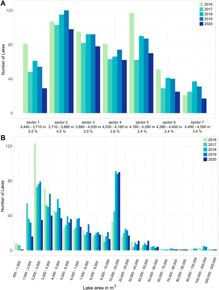
FIGURE 5. (A) Distribution of the number of lakes along the altitude divided into seven sectors. Each sector is specified by its altitude range (m a.s.l.). (B) Distribution of the number of lakes according to their area in m².

The spatial distribution of lakes (Figure 6; Supplementary Figures S2,S3) was highly variable between each of the observation periods. Additionally, the mapping of the inundated area gives an indication of the lake bathymetry, as shown in Figures 6D,E for the Yermanendu Lake in 2018 and 2020.

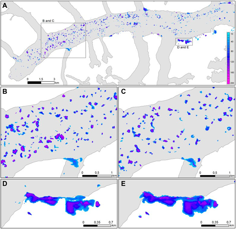
FIGURE 6. Distribution of lakes and duration of water coverage for the complete glacier in 2018 (A), for the second sector (3,710–3,880 m a.s.l.) in 2018 (B) and in 2020 (C), and for the Yermanendu Lake (4,160–4,280 m a.s.l.) in 2018 (D) and in 2020 (E). The color represents the duration of water coverage in days. Pink color means that the pixel was covered with water for 120 days, whereas blue means coverage of 40–50 days. All figures have the same legend shown in (A).

4.4 Seasonal Evolution

The seasonal evolution of the maximum area of all supraglacial lakes (including Yermanendu and Liligo Lakes) for each summer season from 2016 to 2020 is displayed in Figure 7. The equivalent disaggregated data for Yermanendu and Liligo Lakes can be found in Supplementary Figure S4. The lake area evolution can be divided into three distinct stages: 1) in 2016 and 2017, the total lake area remains below 2 km² with a maximum in early June and end-July, respectively, followed by a consistent decrease from early and mid-August onward, 2) 2018 and 2019 were characterized by larger water areas of about 2.5 km² from mid-June to mid-July and a steeper decrease from end-July onward, and 3) in 2020, the lake area peaks at 2.62 km² in early June with a following decrease until mid-August and a short increase from mid-August to mid-September. A consistent characteristic for all 5 years is the rapid lake expansion at the beginning of the ablation season. In 2018, 2019, and 2020, the lake onset had started in mid-April with a continuous increase until mid-June. The years 2016 and 2017 were characterized by a delayed lake onset, starting 1 month later in mid-May. In 2020, the increase in lake area between mid-April and early June is similar in 2018 and 2019, but instead of a constant lake area until mid-July, it decreased. The peak in the lake area from early September to mid-September corresponds well with the dynamics of Yermanendu Lake (Supplementary Figures S4A,B). Data availability reduced the number of observations available in 2016. Consequently, the seasonal evolution could not be sampled with the same high temporal resolution as it was possible for the other years (Supplementary Figure S5).

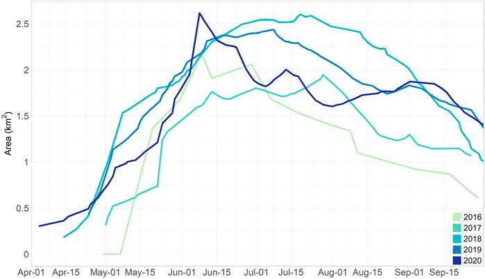
FIGURE 7. Seasonal evolution of the total supraglacial lake area in km² from April to September for 2016 to 2020.

4.5 Probability Density

Figure 8 shows the distribution of lake areas through time and depicts median, interquartile range, and probability density values. The rise of the median lake area from 1.2 in 2016 to 1.7–1.9 in 2018–2020 is clearly visible. The interquartile ranges of 2016 and 2018 showed a larger variation of lake areas than in 2020. The probability density represents the distribution of lake areas and differs each year. The lake area of 2016 was symmetrically distributed, meaning a relatively high variance. In contrast, the lake areas of 2017 and 2019 were bimodal with a more pronounced shape in 2017. The probability density of 2019 had a negative skew indicating that most of the lake areas were larger than the median. In 2020, most of the lake areas were concentrated around the median value. Overall, the probability density data reinforce the observation of there being great year-to-year variability.

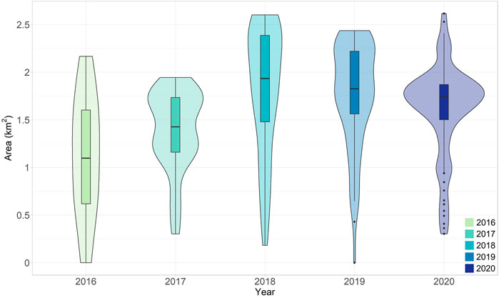
FIGURE 8. Median, interquartile ranges, and probability density of the lake areas of the summertime series for the 5 years presented in a violin plot.

4.6 Seasonal and Trend Components

The seasonal variability in the lake area (Figure 9) largely reflects the pattern depicted in Figure 7, with a yearly maximum being identified in June/July. It is positively skewed, indicating a quick onset of lake formation in spring and slower drainage in the lake area towards autumn. The linear trend component was quantified to 0.16 ± 0.14 km² per year, which corresponds to an increase in the supraglacial lake area of 11.12 ± 9.57% per year. Considering the uncertainty of the linear trend component and the degrees of freedom defined by the number of months of the times series, the linear trend is not significant at the 95% level (p-value 0.125) (Weatherhead et al., 1998; Santer et al., 2000).

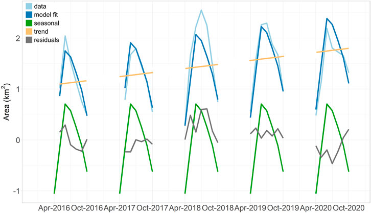
FIGURE 9. Monthly means of the total lake area (data), model fit, seasonal components, linear trend, and residuals for 2016 to 2020. The seasonal component and the residuals are plotted in relative units.

4.7 Precipitation and Temperature

Figure 10 represents the precipitation and temperature in the Standardized Precipitation Index (SPI) and the Standardized Temperature Index (STI) for the period from 2016 to 2020 (McKee et al., 1993). The advantage of using indices (rather than raw data) is the better representation of anomalies. We aggregated both variables over a period of 3 months, as this reflects seasonal-scale deficit and surpluses (Winkler et al., 2017; Wendleder et al., 2018). A significant increase for both indices above 1.0 is observed from 2016 to 2018 and in summer 2019, which represents moderate surpluses. A direct connection between supraglacial lake evolution and climate could not be identified, even though the climate data show a tendency to greater precipitation and higher temperatures in terms of amplitude and time.

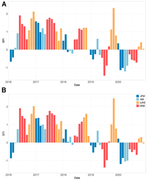
FIGURE 10. SPI (A) and STI (B) from 2016 to 2020 for the monthly precipitation and temperature, color-coded for the seasonal distribution: January, February, and March (JFM) in dark blue, April and May (AM) in light blue, June to September (JJAS) in orange, and October to December (OND) in red. The index values range from −2 to +2, whereas −0.99 to +0.99 indicate near normal, +1.0 to +1.4 moderate surpluses, +1.5 to +1.99 very high surpluses, −1.0 and −1.49 moderate deficits, and −1.5 to −1.99 and $<-$2.0 severe deficits.

5 Accuracy of Supraglacial Lake Areas

Table 4 lists the RSE for all sensors and the multi-temporal time series. Variability in image coverage impeded a direct comparison of the classification accuracy from optical imagery of different dates. It is notable that the reference datasets of July 7, August 6, and August 21 (all 2019) had a higher RSE. These scenes covered the Liligo Lake (7 km) with an area of 0.06 km² (July 22, 2019). From mid-July, Liligo Lake was fed by the meltwater of the Liligo Glacier and hence, the turbidity increased. As turbid water and ice had similar spectral reflectance, the Liligo Lake was consistently misclassified as ice. In the case of the SAR sensors, the classifications derived from descending passes, i.e., glacier velocity parallel to the SAR line of sight, provided better results. However, the mean relative RSE of the multi-temporal time series was at 1.0% (total area of 9.151 km² with an absolute RSE of 0.0945 km²) and showed better accuracy than the mean relative RSE of Sentinel-2, PlanetScope, TerraSAR-X, and Sentinel-1 with 7.1% (total area of 7.483 km² with an absolute RSE of 0.054 km²). Our classification errors are comparable with the error of 2.7% in Liang et al. (2012), 4.5% in Sundal et al. (2009), and 4.0% in Selmes et al. (2011).

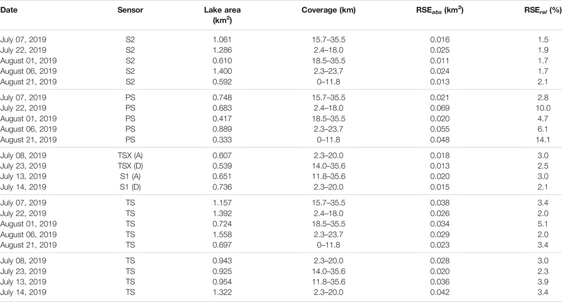
TABLE 4. Accuracy assessment with absolute and relative Root Squared Error (RSE) for Sentinel-2 (S2), PlanetScope (PS), TerraSAR-X (TSX), and Sentinel-1 (S1) for the multi-sensor time series (TS) based on manually digitized reference dataset derived of PlanetScope data from 2019. The lake area referred to the total classified lake area covered by the reference data set of PlanetScope. The coverage of the reference data set was given as distance along the centerline.

6 Discussion

6.1 Comparison With Existing Methods for Supraglacial Lake Classifications

Two previous studies have classified the supraglacial lakes on the Baltoro Glacier, but only for one to three scenes per year. Wendleder et al. (2018) calculated the NDWI based on the green and the near-infrared band for the Landsat-8 Operational Land Imager (OLI) Level-2 data. The threshold for the water detection was empirically determined to be 0.1. Misclassifications like ice-covered surfaces of the tributaries Yermanendu and Biarchedi Glacier and ice sails were manually removed. They detected a total lake area of 2.28 km² on June 04, 2016, 1.83 km² on June 20, 2016, 1.45 km² on September 08, 2016, and 2.09 km² on June 23, 2017. The results of this study differ by −0.28 km², +0.16 km², −0.52 km², and −0.37 km², respectively. The acquisition dates of the time series do not correspond to the Landsat-8 dates; hence, we linearly interpolated to the lake area for better comparison. Since the lake dynamics are highly variable, the linear interpolation could produce differences. Furthermore, the coarser spatial resolution of Landsat-8 of 30 m could lead to a higher lake area (Watson et al., 2018). The greatest discrepancy of +0.52 km² is due to there being only two Sentinel-2 scenes between July and September 2016, neither of which are completely cloud-free, and there being no image pairs of Sentinel-1 and 2 acquired on the same date, which is needed for the calculation of the linear regression. Consequently, the SAR area harmonization employed in the current study could not be applied for all lakes, only for persistent lakes, and the missing lake areas could not be interpolated based on Sentinel-2. Hence, the classification results on September 08, 2016, derived from Sentinel-1 are lower. On the other hand, the lake dynamics shown in 2016 in the previous study, with a high lake area in early June followed by a decrease in lake area, corresponds with our current observation.

The second study mapping supraglacial lakes on Baltoro Glacier used a U-Net model with EfficientNet backbone based on PlanetScope data (Qayyum et al., 2020). Qayyum et al. (2020) classified lake areas of 2.25 km² on July 14, 2017, 1.96 km² on July 27, 2017, 1.83 km² on August 7, 2017, 2.22 km² on July 14 and 15, 2018, and 2.61 km² on July 12–16, 2019. For complete coverage of the glacier surface in 2018 and 2019, they used PlanetScope data acquired within a period of 2 or 4 days. Since the total lake area was constant at both times, the classification results do not contain any seasonal variations. Our results differ by −0.51, −0.02, −0.18, +0.3, and –0.3 km². The differences in the classification results can most likely be accounted for by the different ground samplings. In particular, the data of the multi-sensor time series in our study were sampled to 10 m, whereas the study of Qayyum et al. (2020) was based on the ground sampling of 3 m.

6.2 Relationship Between Supraglacial Lake Evolution and Climate

According to SPI and STI, the years 2016–2017 were influenced by stronger precipitation and higher air temperatures in April and May compared to 2018, 2019, and 2020. As the seasonal lake evolution shows a larger area for 2018, 2019, and 2020, a connection between lake evolution and climate cannot be identified, even though the climate data show a tendency to larger precipitation and higher temperatures in terms of amplitude and time. Satellite images and classification results revealed that newly created supraglacial lakes were mostly fed by precipitation, either directly by rain or delayed via snowmelt in the depressions. The ice-dammed lakes were additionally filled by snowmelt of the adjacent slopes and glacier meltwater. The greater the contribution of glacier meltwater, the more turbid the lake, as is the case at Liligo Lake around the middle or end of July. It appears then that the stronger and earlier precipitation in 2018–2020 caused an increase in the lake area. In 2018, the glacier downstream of Gore and the north exposed slopes near Liligo Lake and Urdukas were unusually snow-free by mid-April. This was 2–4 weeks in advance of other years. Hence, 2018 was affected by higher temperatures leading to an intensified contribution of snow and glacier meltwater at an altitude of about 4,400 m a.s.l. The period July until September 2020 was cloudier than usual, which could indicate a stronger Indian summer monsoon. Therefore, the undulating patterns in Figure 7 can be explained by higher precipitation resulting in short-term lake fluctuations. This observation is supported by several other studies that monitored an intensification of the westerlies, hence leading to an increase of precipitation for the Karakoram (Cannon et al., 2015; Mölg et al., 2017; de Kok et al., 2020). On the other hand, the frequency and duration of heatwaves in Pakistan also increased, mostly affecting the central and southeast regions and less the Himalayan and the Karakoram (Khan et al., 2019). However, for March and April, 2018, high temperatures were recorded as well for Skardu (World Meteorological Organization, 2021). It seems that the heat waves affected the Karakoram, which would be consistent with our observation of an early snowmelt in spring 2018.

7 Opportunities and Limitations

7.1 Multi-Temporal and Multi-Sensor Time Series

The advantage of the presented approach is the usage of a dense multi-temporal and multi-sensor summertime series. Each sensor has advantages and disadvantages, which can be compensated by integrating them into a combined approach. Sentinel-2 provides a continuous, radiometrically stable time series but without daily or sub-daily imaging capability; this can be filled by the high temporal sampling of PlanetScope data. During periods of cloud cover, SAR data provide important information and in view of the amplification of the winter westerlies and the Indian summer monsoon, its usage will likely become essential. In contrast, the disadvantages of the SAR data, i.e., lake area underestimates and missing data from side-looking radar geometry and undulating glacier surface topographies, can be compensated using optical data acquired on the same day. Due to the east-west orientation of the Baltoro Glacier and the broad glacier valley with a width of 3.5 km, the main glacier was not influenced by layover or radar shadow effects in the SAR images. As both ascending and descending acquisitions were acquired with the same incidence angle of 35°, we cannot determine which incidence angle would be more suitable. The images acquired in the descending orbit, i.e., with the SAR line of sight parallel to the glacier flow, mapped the lake shapes better, which confirms the accuracy improvement by 1% (Table 3).

7.2 Semi-Automatic Approach for Supraglacial Lake Detection

Our study shows that optical and SAR data can be used synergistically to monitor the seasonal evolution of supraglacial lakes on debris-covered glaciers. The approach works semi-automatically without the need for manual cloud removal. Manual interaction is only needed to select the Sentinel-1 and 2 and TerraSAR-X training data for the random forest classifier and the adaption of the threshold for the detection of pixel clusters that were misclassified as water. As the threshold was mostly adjusted for the summertime series in 2016 and 2017 with less imagery, this step will become unnecessary with increased data availability. The classification of the PlanetScope data was completely automatic as the selection of the training data was based on the SGLI results. For the Sentinel-2 data, the MAJA atmospheric correction was used. The main feature of MAJA is the use of multi-temporal information contained in the time series to better estimate aerosol optical thickness and correct atmospheric effects (Hagolle et al., 2017). This enables the comparability within the data and potentially supports the use of our training data for supraglacial lake detection on other debris-covered glaciers. However, for a simple supraglacial lake classification based on the classes “debris,” “ice,” and “lake,” the SGLI, presented for the first time in this study, could be applied on cloud-free Sentinel-2 and PlanetScope data without any previous knowledge.

8 Conclusion

To study the variability of supraglacial lakes on the Baltoro Glacier, we developed a semi-automatic approach based on multi-sensor and multi-temporal summertime series from 2016 to 2020 acquired by the optical sensors Sentinel-2 and PlanetScope and the SAR sensors Sentinel-1 and TerraSAR-X. Our study showed that the supraglacial lakes filled between mid-April to mid-June and drained between mid-June to mid-September. In all cases, lake areas expanded faster than they contracted. The five-year study period showed that the total lake area varied from year to year, with the largest total lake area in 2018 (5.783 km²) and the smallest lake area in 2017 (3.563 km²). Variations in the total number of lakes were not recognizable, though there was a tendency towards creating larger lakes (>0.04 km²) over time. The local distribution of the lakes densified, especially in the glacier section between 3,710 m and 3,880 m a.s.l. The percentage of lake area (as a component of overall glacier area) rose by 3.3% between 2017 and 2018. The supraglacial lakes were mostly fed by precipitation either directly with rainfall or time delayed via snowmelt in the hummocks. The ice-marginal lakes (Yermanendu and Liligo) were additionally filled by snowmelt derived from adjacent slopes and glacier meltwater. A linear trend of 11.12 ± 9.57% per year was derived that indicates a possible increase in the lake area. This is supported by pronounced positive anomalies of the SPI and STI during the observation period. However, we conclude that the time series need to be extended in order to identify significant signals. In addition, the connection to climate parameters and oscillations demands further process-based analysis. We anticipate that the rising trend of the supraglacial lake area will continue due to climate change and the accompanying rise in air temperature and intensification of precipitation, which underlines the importance of evaluating continuous time series and thus the use of semi-automated processors.

Data Availability Statement

The original contributions presented in the study are included in the article/Supplementary Material; further inquiries can be directed to the corresponding author.

Author Contributions

AW, AS, CM, and MB designed the research. AW analyzed the data and results and wrote the manuscript. AS helped with the methodology. TE calculated the seasonal and trend components and wrote Section 3.5 and Section 4.6. PD processed the MAJA corrected Sentinel-2 data. All authors helped to edit and to improve the manuscript.

Conflict of Interest

The authors declare that the research was conducted in the absence of any commercial or financial relationships that could be construed as a potential conflict of interest.

Publisher’s Note

All claims expressed in this article are solely those of the authors and do not necessarily represent those of their affiliated organizations, or those of the publisher, the editors and the reviewers. Any product that may be evaluated in this article, or claim that may be made by its manufacturer, is not guaranteed or endorsed by the publisher.

Acknowledgments

The authors acknowledge the use of TerraSAR-X data (©DLR 2019-2020), Sentinel-1 and 2 data (©ESA 2019-2020) provided by DLR PAC/LTA, PlanetScope data (©Planet 2019-2020), and ERA5-Land provided by Copernicus Climate Change Service (C3S) Climate Data Store (CDS). We would like to thank Duncan Quincey, Adina Elena Racoviteanu, and Qiao Liu for their corrections that helped to strengthen the manuscript.

Supplementary Material

The Supplementary Material for this article can be found online at: https://www.frontiersin.org/articles/10.3389/feart.2021.725394/full#supplementary-material

References

Airbus (2020). Copernicus Digital Elevation Model Product Handbook RFP/RFI-No.: AO/1-9422/18/I-LG, Version: 2.1. https://spacedata.copernicus.eu/documents/20126/0/GEO1988-CopernicusDEM-SPE-002_ProductHandbook_I1.00.pdf/082dd479-f908-bf42-51bf-4c0053129f7c?t=1586526993604.
Anderson, L. S., and Anderson, R. S. (2019). Modeling Debris-Covered Glaciers: Response to Steady Debris Deposition. Cryosphere 10, 1105–1124. doi:10.5194/tc-10-1105-2016
Benn, D. I., Bolch, T., Hands, K., Gulley, J., Luckman, A., Nicholson, L. I., et al. (2012). Response of Debris-Covered Glaciers in the Mount everest Region to Recent Warming, and Implications for Outburst Flood Hazards. Earth Sci. Rev. 114, 156–174. doi:10.1016/j.earscirev.2012.03.008
Benn, D. I., Thompson, S., Gulley, J., Mertes, J., Luckman, A., and Nicholson, L. (2017). Structure and Evolution of the Drainage System of a Himalayan Debris-Covered Glacier, and its Relationship with Patterns of Mass Loss. Cryosphere 11, 2247–2264. doi:10.5194/tc-11-2247-2017
Bolch, T., Kulkarni, A., Kääb, A., Huggel, C., Paul, F., Cogley, J. G., et al. (2012). The State and Fate of Himalayan Glaciers. Science 336, 310–314. doi:10.1126/science.1215828
Bookhagen, B., and Burbank, D. W. (2006). Topography, Relief, and TRMM-Derived Rainfall Variations along the Himalaya. Geophys. Res. Lett. 33, 1–5. doi:10.1029/2006GL026037
Brun, F., Wagnon, P., Berthier, E., Shea, J. M., Immerzeel, W. W., Kraaijenbrink, P. D. A., et al. (2018). Ice Cliff Contribution to the Tongue-wide Ablation of Changri Nup Glacier, nepal, central Himalaya. Cryosphere 12, 3439–3457. doi:10.5194/tc-12-3439-2018
Buri, P., Miles, E. S., Steiner, J. F., Ragettli, S., and Pellicciotti, F. (2021). Supraglacial Ice Cliffs Can Substantially Increase the Mass Loss of Debris‐Covered Glaciers. Geophys. Res. Lett. 48, 1–11. doi:10.1029/2020gl092150
Cannon, F., Carvalho, L. M. V., Jones, C., and Bookhagen, B. (2015). Multi-annual Variations in winter westerly Disturbance Activity Affecting the Himalaya. Clim. Dyn. 44, 441–455. doi:10.1007/s00382-014-2248-8
Collier, E., Maussion, F., Nicholson, L. I., Mölg, T., Immerzeel, W. W., and Bush, A. B. G. (2015). Impact of Debris Cover on Glacier Ablation and Atmosphere-Glacier Feedbacks in the Karakoram. Cryosphere 9, 1617–1632. doi:10.5194/tc-9-1617-2015
Cooley, S., Smith, L., Stepan, L., and Mascaro, J. (2017). Tracking Dynamic Northern Surface Water Changes with High-Frequency Planet Cubesat Imagery. Remote Sensing 9, 1306–1321. doi:10.3390/rs9121306
Davies, E. R. (2005). “Basic Image Filtering Operations,” in Signal Processing and its Applications. Editor E. Davies. Third Edition (Burlington: Morgan Kaufmann), 47–101. doi:10.1016/b978-012206093-9/50006-x
de Jonge, E., and van der Loo, M. (2013). An Introduction to Data Cleaning with R. The Hague: Statistics Netherlands.
de Kok, R. J., Kraaijenbrink, P. D. A., Tuinenburg, O. A., Bonekamp, P. N. J., and Immerzeel, W. W. (2020). Towards Understanding the Pattern of Glacier Mass Balances in High Mountain Asia Using Regional Climatic Modelling. Cryosphere 14, 3215–3234. doi:10.5194/tc-14-3215-2020
Dobreva, I., Bishop, M., and Bush, A. (2017). Climate-Glacier Dynamics and Topographic Forcing in the Karakoram Himalaya: Concepts, Issues and Research Directions. Water 9, 405–429. doi:10.3390/w9060405
Eineder, M., and Fritz, T. (2009). TerraSAR-X Ground Segment Basic Product Specification Document; Doc: TX-GS-DD-3302. Wessling, Germany: German Aerospace Center (DLR). https://tandemx-science.dlr.de/pdfs/TX-GS-DD-3302_Basic-Products-Specification-Document_V1.9.pdf.
Evatt, G. W., Mayer, C., Mallinson, A., Abrahams, I. D., Heil, M., and Nicholson, L. (2017). The Secret Life of Ice Sails. J. Glaciol. 63, 1049–1062. doi:10.1017/jog.2017.72
Haberäcker, P. (1987). Digitale Bildverarbeitung; Grundlagen und Anwendungen. Muenchen, Wien: Hanser.
Hagolle, O., Huc, M., Desjardins, C., Auer, S., and Richter, R. (2017). Maja Algorithm Theoretical Basis Document. Stochastic Environ. Res. Risk Assess. Version 1.0, 1–40. doi:10.5281/zenodo.1209633
Hersbach, H., Bell, B., Berrisford, P., Hirahara, S., Horányi, A., Muñoz‐Sabater, J., et al. (2020). The Era5 Global Reanalysis. Q.J.R. Meteorol. Soc. 146, 1999–2049. doi:10.1002/qj.3803
Hewitt, K. (2011). Glacier Change, Concentration, and Elevation Effects in the Karakoram Himalaya, Upper Indus basin. Mountain Res. Develop. 31, 188–200. doi:10.1659/MRD-JOURNAL-D-11-00020.1
Houborg, R., and McCabe, M. (2016). High-resolution Ndvi from Planet’s Constellation of Earth Observing Nano-Satellites: A New Data Source for Precision Agriculture. Remote Sensing 8, 1–19. doi:10.3390/rs8090768
Huo, D., Bishop, M. P., and Bush, A. B. G. (2021). Understanding Complex Debris-Covered Glaciers: Concepts, Issues, and Research Directions. Front. Earth Sci. 9, 358. doi:10.3389/feart.2021.652279
Khan, N., Shahid, S., Ismail, T., Ahmed, K., and Nawaz, N. (2019). Trends in Heat Wave Related Indices in pakistan. Stoch Environ. Res. Risk Assess. 33, 287–302. doi:10.1007/s00477-018-1605-2
Kraaijenbrink, P., Meijer, S. W., Shea, J. M., Pellicciotti, F., De Jong, S. M., and Immerzeel, W. W. (2016). Seasonal Surface Velocities of a Himalayan Glacier Derived by Automated Correlation of Unmanned Aerial Vehicle Imagery. Ann. Glaciol. 57, 103–113. doi:10.3189/2016AoG71A072
Liang, Y.-L., Colgan, W., Lv, Q., Steffen, K., Abdalati, W., Stroeve, J., et al. (2012). A Decadal Investigation of Supraglacial Lakes in West greenland Using a Fully Automatic Detection and Tracking Algorithm. Remote Sensing Environ. 123, 127–138. doi:10.1016/j.rse.2012.03.020
Qiao, L., Mayer, C., and Liu, S. (2015). Distribution and Interannual Variability of Supraglacial Lakes on Debris-Covered Glaciers in the Khan Tengri-Tumor Mountains, central Asia. Environ. Res. Lett. 10, 014014. doi:10.1088/1748-9326/10/1/014014
Mayer, C., Lambrecht, A., Belò, M., Smiraglia, C., and Diolaiuti, G. (2006). Glaciological Characteristics of the Ablation Zone of Baltoro Glacier, Karakoram, pakistan. Ann. Glaciol. 43, 123–131. doi:10.3189/172756406781812087
McFeeters, S. K. (1996). The Use of the Normalized Difference Water Index (NDWI) in the Delineation of Open Water Features. Int. J. Remote Sensing 17, 1425–1432. doi:10.1080/01431169608948714
McKee, T. B., Doesken, N. J., and Kleist, J. (1993). “The Relationship of Drought Frequency and Duration to Time Scales,” in Proceedings of the 8th Conference on Applied Climatology. Anaheim, January 17-22, 1993, 179–183.
Mihalcea, C., Mayer, C., Diolaiuti, G., D’Agata, C., Smiraglia, C., Lambrecht, A., et al. (2008). Spatial Distribution of Debris Thickness and Melting from Remote-Sensing and Meteorological Data, at Debris-Covered Baltoro Glacier, Karakoram, pakistan. Ann. Glaciol. 48, 49–57. doi:10.3189/172756408784700680
Miles, E. S., Willis, I. C., Arnold, N. S., Steiner, J., and Pellicciotti, F. (2017a). Spatial, Seasonal and Interannual Variability of Supraglacial Ponds in the Langtang Valley of Nepal, 1999-2013. J. Glaciol. 63, 88–105. doi:10.1017/jog.2016.120
Miles, K. E., Willis, I. C., Benedek, C. L., Williamson, A. G., and Tedesco, M. (2017b). Toward Monitoring Surface and Subsurface Lakes on the greenland Ice Sheet Using sentinel-1 Sar and Landsat-8 Oli Imagery. Front. Earth Sci. 5, 58. doi:10.3389/feart.2017.00058
Miles, E. S., Willis, I., Buri, P., Steiner, J. F., Arnold, N. S., and Pellicciotti, F. (2018). Surface Pond Energy Absorption across Four Himalayan Glaciers Accounts for 1/8 of Total Catchment Ice Loss. Geophys. Res. Lett. 45, 10464–10473. doi:10.1029/2018GL079678
Miles, K. E., Hubbard, B., Irvine-Fynn, T. D. L., Miles, E. S., Quincey, D. J., and Rowan, A. V. (2020). Hydrology of Debris-Covered Glaciers in High Mountain Asia. Earth Sci. Rev. 207, 103212. doi:10.1016/j.earscirev.2020.103212
Mölg, T., Maussion, F., Collier, E., Chiang, J. C. H., and Scherer, D. (2017). Prominent Midlatitude Circulation Signature in High Asia's Surface Climate during Monsoon. J. Geophys. Res. Atmos. 122, 12702–12712. doi:10.1002/2017JD027414
Mölg, N., Ferguson, J., Bolch, T., and Vieli, A. (2020). On the Influence of Debris Cover on Glacier Morphology: How High-Relief Structures Evolve from Smooth Surfaces. Geomorphology 357 (12), 702–712. doi:10.1002/2017JD027414
Muñoz-Sabater, J. (2019). Era5-land Hourly Data from 1981 to Present. Copernicus Climate Change Service (C3s) Climate Data Store (Cds). doi:10.24381/cds.e2161bac
Nicholson, L., and Benn, D. I. (2006). Calculating Ice Melt beneath a Debris Layer Using Meteorological Data. J. Glaciol. 52, 463–470. doi:10.3189/172756506781828584
Nicholson, L. I., McCarthy, M., Pritchard, H. D., and Willis, I. (2018). Supraglacial Debris Thickness Variability: Impact on Ablation and Relation to Terrain Properties. Cryosphere 12, 3719–3734. doi:10.5194/tc-12-3719-2018
Ostrem, G. (1959). Ice Melting under a Thin Layer of Moraine, and the Existence of Ice Cores in Moraine Ridges. Geografiska Annaler 41, 228–230. doi:10.1080/20014422.1959.11907953
PlanetScope (2020). Planet Imagery Product Specification. San Francisco, CA: Planet Labs, Inc. https://assets.planet.com/docs/Planet_Combined_Imagery_Product_Specs_letter_screen.pdf.
Qayyum, N., Ghuffar, S., Ahmad, H., Yousaf, A., and Shahid, I. (2020). Glacial Lakes Mapping Using Multi Satellite Planetscope Imagery and Deep Learning. ISPRS Int. J. Geo. Inform. 9, 1–23. doi:10.3390/ijgi9100560
Quincey, D. J., Richardson, S. D., Luckman, A., Lucas, R. M., Reynolds, J. M., Hambrey, M. J., et al. (2007). Early Recognition of Glacial lake Hazards in the Himalaya Using Remote Sensing Datasets. Glob. Planet. Change 56, 137–152. doi:10.1016/j.gloplacha.2006.07.013
Quincey, D. J., Copland, L., Mayer, C., Bishop, M., Luckman, A., and Belò, M. (2009). Ice Velocity and Climate Variations for Baltoro Glacier, pakistan. J. Glaciol. 55, 1061–1071. doi:10.3189/002214309790794913
Reynolds, J. M. (2006). Role of Geophysics in Glacial hazard Assessment. First Break 24, 61–66. doi:10.3997/1365-2397.24.8.27068
Rosin, P. L. (2001). Unimodal Thresholding. Pattern Recognition 34, 2083–2096. doi:10.1016/S0031-3203(00)00136-9
Roth, A. (2019). Methoden zur Schattendetektion und -entfernung zur Verbesserten Landbedeckungsklassifikation im Untersuchungsgebiet Berchtesgadener Land anhand von Sentinel-2 Daten. Bachelorarbeit. Hochschule München-Kartographie, Geomedientechnik.
Rowan, A. V., Egholm, D. L., Quincey, D. J., and Glasser, N. F. (2015). Modelling the Feedbacks between Mass Balance, Ice Flow and Debris Transport to Predict the Response to Climate Change of Debris-Covered Glaciers in the Himalaya. Earth Planet. Sci. Lett. 430, 427–438. doi:10.1016/j.epsl.2015.09.004
Sakai, A., and Fujita, K. (2010). Formation Conditions of Supraglacial Lakes on Debris-Covered Glaciers in the Himalaya. J. Glaciol. 56, 177–181. doi:10.3189/002214310791190785
Sakai, A. (2012). Glacial Lakes in the Himalayas: a Review on Formation and Expansion Processes. Glob. Environ. Res., 23–30.
Santer, B. D., Wigley, T. M. L., Boyle, J. S., Gaffen, D. J., Hnilo, J. J., Nychka, D., et al. (2000). Statistical Significance of Trends and Trend Differences in Layer-Average Atmospheric Temperature Time Series. J. Geophys. Res. 105, 7337–7356. doi:10.1029/1999JD901105
Scherler, D., Bookhagen, B., and Strecker, M. R. (2011). Spatially Variable Response of Himalayan Glaciers to Climate Change Affected by Debris Cover. Nat. Geosci. 4, 156–159. doi:10.1038/NGEO1068
Schmitt, A., Wendleder, A., and Hinz, S. (2015). The Kennaugh Element Framework for Multi-Scale, Multi-Polarized, Multi-Temporal and Multi-Frequency SAR Image Preparation. ISPRS J. Photogram. Remote Sensing 102, 122–139. doi:10.1016/j.isprsjprs.2015.01.007
Schmitt, A., Wendleder, A., Kleynmans, R., Hell, M., Roth, A., and Hinz, S. (2020). Multi-source and Multi-Temporal Image Fusion on Hypercomplex Bases. Remote Sensing 12, 943–2096. doi:10.3390/rs12060943
Selmes, N., Murray, T., and James, T. D. (2011). Fast Draining Lakes on the greenland Ice Sheet. Geophys. Res. Lett. 38, 1–5. doi:10.1029/2011GL047872
Sundal, A. V., Shepherd, A., Nienow, P., Hanna, E., Palmer, S., and Huybrechts, P. (2009). Evolution of Supra-glacial Lakes across the greenland Ice Sheet. Remote Sensing Environ. 113, 2164–2171. doi:10.1016/j.rse.2009.05.018
Thayyen, R. J., and Gergan, J. T. (2010). Role of Glaciers in Watershed Hydrology: a Preliminary Study of a "Himalayan Catchment". Cryosphere 4, 115–128. doi:10.5194/tc-4-115-2010
Thompson, S., Benn, D. I., Mertes, J., and Luckman, A. (2016). Stagnation and Mass Loss on a Himalayan Debris-Covered Glacier: Processes, Patterns and Rates. J. Glaciol. 62, 467–485. doi:10.1017/jog.2016.37
Vincent, P., Bourbigot, M., Johnsen, H., and Piantanida, R. (2019). Sentinel-1 Product Specification.
Watson, C. S., Quincey, D. J., Carrivick, J. L., and Smith, M. W. (2016). The Dynamics of Supraglacial Ponds in the everest Region, central Himalaya. Glob. Planet. Change 142, 14–27. doi:10.1016/j.gloplacha.2016.04.008
Watson, C. S., King, O., Miles, E. S., and Quincey, D. J. (2018). Optimising Ndwi Supraglacial Pond Classification on Himalayan Debris-Covered Glaciers. Remote Sensing Environ. 217, 414–425. doi:10.1016/j.rse.2018.08.020
Weatherhead, E. C., Reinsel, G. C., Tiao, G. C., Meng, X.-L., Choi, D., Cheang, W.-K., et al. (1998). Factors Affecting the Detection of Trends: Statistical Considerations and Applications to Environmental Data. J. Geophys. Res. 103, 17149–17161. doi:10.1029/98jd00995
Wendleder, A., Friedl, P., and Mayer, C. (2018). Impacts of Climate and Supraglacial Lakes on the Surface Velocity of Baltoro Glacier from 1992 to 2017. Remote Sensing 10, 1681. doi:10.3390/rs10111681
Winkler, K., Gessner, U., and Hochschild, V. (2017). Identifying Droughts Affecting Agriculture in Africa Based on Remote Sensing Time Series between 2000-2016: Rainfall Anomalies and Vegetation Condition in the Context of ENSO. Remote Sensing 9, 831–927. doi:10.3390/rs9080831
World Meteorological Organization (2021). Available at: https://public.wmo.int/en/media/news/march-3rd-warmest-record-many-contrasts (Accessed 05 29, 2021).
Keywords: supraglacial lake, ice-dammed lake, Baltoro Glacier, remote sensing, summertime series, multi-sensor, multi-temporal
Citation: Wendleder A, Schmitt A, Erbertseder T, D’Angelo P, Mayer C and Braun MH (2021) Seasonal Evolution of Supraglacial Lakes on Baltoro Glacier From 2016 to 2020. Front. Earth Sci. 9:725394. doi: 10.3389/feart.2021.725394
Received: 15 June 2021; Accepted: 19 November 2021;
Published: 24 December 2021.
Edited by:
Duncan Joseph Quincey, University of Leeds, United KingdomReviewed by:
Adina Elena Racoviteanu, University of Exeter, United KingdomQiao Liu, Institute of Mountain Hazards and Environment (CAS), China
Copyright © 2021 Wendleder, Schmitt, Erbertseder, D’Angelo, Mayer and Braun. This is an open-access article distributed under the terms of the Creative Commons Attribution License (CC BY). The use, distribution or reproduction in other forums is permitted, provided the original author(s) and the copyright owner(s) are credited and that the original publication in this journal is cited, in accordance with accepted academic practice. No use, distribution or reproduction is permitted which does not comply with these terms.
*Correspondence: Anna Wendleder, anna.wendleder@dlr.de