Bayesian Inference of Ice Softness and Basal Sliding Parameters at Langjökull

1. Introduction

The dynamics of glaciers have become of greater scientific interest in recent times due to global climate change and its impact on the size and flow of glaciers; perhaps most crucially, melting glaciers have an effect on sea levels (Björnsson et al., 2006; Zammit-Mangion et al., 2014; Hock et al., 2019). Glacial dynamics are dependent on two main physical parameters: ice softness, related to the deformation of ice, and basal sliding, related to basal velocity (Cuffey and Paterson, 2010). Both ice softness and basal sliding parameters cannot be measured directly and must be estimated in order to properly understand glacial dynamics and, consequently, globally relevant phenomena such as sea level rise. The purpose of this paper is to use surface velocity data in combination with Bayesian statistical inference in order to infer ice softness and basal sliding parameters, with particular application to Langjökull, a prominent Icelandic glacier (Björnsson, 2017). Iceland, about 10 percent of whose area is covered by glaciers (Björnsson and Pálsson, 2008), is a natural laboratory for cryosphere science, particularly in an era of increasing temperatures and glacial melting.

A simplified definition of a glacier is a mass of ice that is situated upon bedrock or sediment, where ice is accreted from compacted snowfall and is lost due to melting. Ice slowly flows in the direction of the negative gradient of the glacier surface. The flow is thought to be a combination of deformation of the ice due to gravity and sliding of the glacier at the bed. For glaciers that are temperate such as Langjökull, ice softness, which governs the rate of ice deformation, is also constant because softness is dependent on temperature. In contrast, the basal sliding parameter can vary both spatially and temporally, especially during glacial surge events (Björnsson et al., 2003).

We employ Bayesian statistical modeling of surface velocities in order to obtain posterior distributions for ice softness and basal sliding parameters; as such, the approach allows for uncertainty quantification of these pivotal glaciological quantities. Bayesian inference has appeared in the glaciology literature before, albeit for different aims. For instance, Brinkerhoff et al. (2016) use Bayesian inference to estimate subglacial topography, while Werder et al. (2020) and Guan et al. (2016) use Bayesian inference to estimate ice thickness, and Minchew et al. (2015) use Bayesian methods to infer velocity fields from multiple repeat-pass interferometric synthetic aperture radar (InSAR) measurements in Iceland. Petra et al. (2014) and Isaac et al. (2015) develop computationally efficient methods for inverse problems involving ice-sheet models, within a Bayesian framework. Perhaps the closest Bayesian inference papers in the literature to the work described here are in Pralong and Gudmundsson (2011) and Raymond and Gudmundsson (2009), which use Bayesian inference to estimate basal sliding and basal topography properties jointly. Building off of this work, we infer ice softness and basal sliding parameters jointly, and infer posterior probability distributions for ice softness and basal sliding parameters. In many instances subglacial topography is not known and must be inferred, but in the case of Langjökull basal topography is known due to the radio-echo survey of the bed Björnsson and Pálsson (2020) and surface elevation topography maps from various sources are also available (Pálsson et al., 2012).

An important result is that the estimated value of ice softness is comparable to the recommended value for temperate glaciers from Cuffey and Paterson (2010), despite that a nearly flat prior is used. In contrast to the previous works, the Bayesian estimate also comes with an uncertainty estimate, here represented with the posterior standard deviation. The posterior is substantially more precise (i.e., lower standard deviation) than the prior, suggesting that the learning of physical parameters is achieved. The inferred spatial variation in basal sliding appears to be consistent with prior work on characterizing horizontal velocities at Langjökull (Minchew et al., 2015).

The structure of the paper is as follows. In section 2, we begin with an overview of the equations that are used to relate ice softness and basal sliding parameters to glacier surface velocities computed with the shallow ice approximation of the stress balance, as derived in Marshall et al. (2005). A detailed description of Bayesian statistical models of surface velocity and an explanation of the Gibbs sampler (i.e., a Markov chain Monte Carlo approach for sampling from the posterior distribution) that is used for inference of physical parameters follows. Additionally, we describe the surface elevation, bed topography, and surface velocity data from the University of Iceland Institute of Earth Sciences (UI-IES). Section 3 discusses the results of applying the Bayesian statistical models to the Langjökull data. Section 4 discusses these results in a more general glaciological context, points out limitations of the approach, and suggests future avenues for work. While the focus of this paper is Langjökull, the delineated approach can be applied to other glaciers where data on surface velocity, bed, and surface topography are available, and the SIA is appropriate. The melting of such glaciers is expected to contribute to the rise of sea levels within the next century, supporting the scientific importance of the statistical modeling and inference within this paper.

2. Method

The Bayesian statistical models that are used in this analysis involve a shallow ice approximation (SIA) model for glacier surface velocity in 2 horizontal dimensions. The probability distributions for surface velocity data use these equations and take either a normal or t distribution. Prior distributions are used for the ice softness and basal sliding parameters, and a Markov chain Monte Carlo (MCMC) algorithm known as Gibbs sampling is used to conduct posterior inference. In the following subsections, we discuss these matters in more depth, and conclude with a description of the data sources that we apply the Bayesian statistical modeling and methodology to. We refer the reader to the Appendix, section 5, for further mathematical equations and details.

2.1. Review of Exact Shallow Ice Approximation Surface Velocity Equations

We use an analytically exact SIA model for horizontal velocities without longitudinal coupling, as in Equation (12) of section 2.2 of Marshall et al. (2005), a section which presents the derivation of the SIA for a 2 dimensional model. The SIA is valid when the thickness of a glacier is much less than horizontal dimensions, as occurs at Langjökull (Björnsson and Pálsson, 2008). A SIA (Hutter, 1983) is a commonly used physical model for shallow glacial dynamics as for instance in Marshall et al. (2005), Bueler et al. (2005), Jarosch et al. (2013), and Gopalan et al. (2018), to give a few examples. A SIA has been applied specifically to Langjökull in Flowers et al. (2007), for instance. By x and y directions, we are referring to their typical usage in a Cartesian coordinate system. In particular, Marshall et al. (2005) show that the exact surface velocities in the x and y directions, v_x and v_y respectively, are given by:

In the above equations, B is the constant ice-softness parameter and γ(x, y, t) is the basal sliding field parameter, which varies spatially and temporally. Additionally, ρ is the density of ice, g is gravitational acceleration, n is a constant from the constitutive relation for temperate ice that is typically set to 3 (and is precisely 3 in this paper), and H(x, y, t) is glacial thickness.

Furthermore, if S(x, y, t) denotes the glacier surface elevation, basal shear stress is given by:

and α is the surface slope, given by:

As such, glacial flow under this model is in the direction of the negative surface gradient, the $-\frac{\partial S}{\partial x}$ and $-\frac{\partial S}{\partial y}$ terms.

2.2. Bayesian Statistical Models for Surface Velocities

We construct and use Bayesian statistical models that allow for the inference of ice softness and basal sliding parameters. The models have two important pieces – the first relates the analytical SIA surface velocities, v_x and v_y, which in turn depend on the physical parameters B and γ, to the observed surface velocity data. The second important aspect of the Bayesian model is the prior distribution for parameters. In the next few subsections we describe both the data distributions and prior distributions, and follow up with how Bayesian inference is conducted computationally.

2.2.1. Normal Distribution for Surface Velocities

We first consider a normal distribution (i.e., a normal model) for surface velocity data. Specifically, the observed velocity in the x direction for a particular site i with spatio-temporal coordinates (x_i, y_i, t_i) is a normal distribution with mean v_x(B, γ(x_i, y_i, t_i)) and standard deviation σ_x. Likewise, the observed surface velocity in the y direction for a particular site i at time t is also normally distributed with mean v_y(B, γ(x_i, y_i, t_i)) and standard deviation σ_y. Expressions for v_x and v_y are given in Equations (2.1) and (2.2). Independence is assumed between x and y velocity components for a given site and between distinct sites. A Kendall correlation test between x and y velocity components fails to reject the assumption of no correlation with the data, which is consistent with the assumption of independence between x and y surface velocity components. The reader is referred to section 5, the Appendix, for a precise mathematical specification.

2.2.2. t Distribution for Surface Velocities

We next consider a t distribution (i.e., a t model) for surface velocity data. That is, the observed velocity in the x direction for a particular site i with spatio-temporal coordinates (x_i, y_i, t_i) is t distributed, with mean v_x(B, γ(x_i, y_i, t_i)) and scale σ_x. To accommodate heavy-tailed deviations from the SIA mean, we use a small degrees of freedom parameter: 3.0001. This choice of degrees of freedom allows for heavy tails (heaviness of tails increases with decreasing degrees of freedom) and maintains a well-defined skewness (skewness is undefined for degrees of freedom less than or equal to 3). Likewise, the velocity in y direction for a particular site is also t distributed with mean v_y(B, γ(x_i, y_i, t_i)) and scale σ_y. As with the normal distribution model, independence is assumed between x and y velocity components for a given site and between distinct sites. As discussed in the previous section, a Kendall correlation test between x and y surface velocity components fails to reject the assumption of no correlation with the data set, which is consistent with the assumption of independence between x and y velocity components. The reader is referred to the Appendix (Section 5) for a precise mathematical specification.

2.2.3. Prior Distributions for Physical Parameters

A normal distribution with mean 35 and standard deviation 30 that is truncated to be on the interval [1, 70] is used for the ice-softness parameter (units are 10⁻²⁵s⁻¹Pa⁻³); this is a nearly flat prior on the interval [1,70] (see comparison of the prior and posterior in the next section) that encapsulates a range of temperate ice softness values presented in Cuffey and Paterson (2010) (24, 38, and 55 in units of 10⁻²⁵s⁻¹Pa⁻³) based on ice-softness measurements. Additionally, the prior distribution for logγ follows a Gaussian process distribution with mean 0 and Matérn kernel for the covariance, where correlation is a decreasing function of Euclidean spatial distance between measurements. Specific mathematical equations for all priors are given in the Appendix (section 5).

We use the parameterization logγ so that a Gaussian process prior is sensible: a Gaussian process prior for γ would still allow for spatial correlation but admit negative values for γ, which is not physically plausible. The Matérn kernel is commonly used for geostatistical applications (Gelfand et al., 2010; Bakka et al., 2018) and subsumes both the exponential and Gaussian kernels, widely used for Gaussian processes. Specifically, a smoothness parameter of 0.5 corresponds to exponential and a smoothness parameter that approaches infinity corresponds to Gaussian. In this work, smoothness and range parameters of the Matérn kernel are selected by minimizing the posterior predictive mean absolute error over the set {100, 1000, 10000} for the range and {0.5, 2, 10} for the smoothness. Based on this criterion, a range of 100 is used for the normal and t distribution Bayesian models; the smoothness is 10 for the t distribution Bayesian model and 0.5 for the normal distribution Bayesian model. The marginal variance is set to 100, which is large enough such that sensible values of basal sliding (i.e., correct order of magnitude) are within one to two standard deviations of the mean. The prior sensitivity analysis in the Appendix (section 5) examines when priors are changed using an inverse-gamma prior (which is not truncated) for B as well as a smaller marginal variance for the Gaussian process prior for logγ. The results indicate that the posterior is not substantially affected by changing the prior distributions.

2.2.4. Posterior Distribution and Inference via Gibbs Sampling

The overarching aim of this Bayesian analysis is to sample from the posterior distribution of B, logγ, σ_x, and σ_y, which by Bayes' theorem is:

In the above expression, the x surface velocity measurements at N sites are denoted by $Y_x\in {ℝ}^N$, and the y surface velocity measurements are denoted by $Y_y\in {ℝ}^N$. The posterior samples of B and logγ are substituted into Equations (2.1) and (2.2) for v_x and v_y to generate posterior samples of the x and y velocities.

The posterior distribution is not analytically tractable, and a Markov chain Monte Carlo algorithm (MCMC) is often used to sample from the posterior distribution in such a scenario (Tierney, 1994). Specifically, we develop a Gibbs sampling approach to sample from the posterior distribution. The idea of the Gibbs sampling approach is to sequentially sample from the posterior distribution of each parameter conditional on the data and remaining parameters: p(B|−), p(logγ|−), p(σ_x|−), and p(σ_y|−), where - indicates all other variables and data. If this is iterated for many steps, the samples will be drawn from the posterior distribution, p(B, logγ, σ_x, σ_y|Y_x, Y_y). Section 5 contains the precise Gibbs sampler steps that are run iteratively.

The Gibbs sampler crucially relies on an elliptical slice sampling step for logγ. Instead of sampling from each component of logγ one-by-one for each of the N sites (which is usually computationally inefficient), we use elliptical slice sampling because of the Gaussian process prior on logγ. Elliptical slice sampling (Murray et al., 2010) is an extension of slice sampling (Neal, 2003) that is designed to sample from a posterior distribution in which the prior distribution is a Gaussian process. This property holds since logγ has a Gaussian process prior. The algorithm is shown to be a competitive alternative to Metropolis-Hastings (Tierney, 1994) for Gaussian process priors, often times working better for real data in terms of a larger effective sample size of Monte Carlo output per unit compute time (Murray et al., 2010).

400,000 posterior samples are drawn from the posterior of physical parameters using Gibbs sampling for both the normal and t distribution variations, after removing a burn in of 50,000 iterations from 450,000 total iterations. The effective sample size and $\widehat{R}$ convergence diagnostic from Vats and Knudson (2018), a recent version of the convergence diagnostic from Gelman and Rubin (1992), provide evidence of convergence of Gibbs sampling; these results are detailed in section 5.

2.3. Langjökull Data

The models set forth in the previous section are applied to Langjökull, which is Iceland's second largest temperate glacier by area (and third by volume) (Björnsson and Pálsson, 2008). Langjökull is 900 km² in area, 190 km³ in volume, 210 m mean thickness, and has a max thickness of about 650 m. In particular, we use:

• 100 m resolution surface elevation topography maps of Langjökull at 1997 (Pálsson et al., 2012), 2007 (Pope et al., 2016), and 2015 (Porter et al., 2018).

• 100 m resolution topography map of the Langjökull glacier bed, constructed from radio echo sounding profiles, nearly 1 km apart, surveyed in 1997 (Björnsson and Pálsson, 2020).

• 51 GPS surface velocity measurements taken across Langjökull at 1997, 2007, and 2015, including (x, y, t) covariates. The UI-IES takes measurements twice a year: once in late spring (end of April to beginning of May) for winter mass balance measurements and once in the fall for summer balance measurements (end of September to mid-October). The displacement measured between the two yearly measurements divided by time yields an estimate of the horizontal surface velocity at a particular measurement site during the summer time, when basal sliding is expected to have a substantial role in velocity (Minchew et al., 2015). A topographical map of Langjökull with the surface velocity survey sites is included in Figure 1.

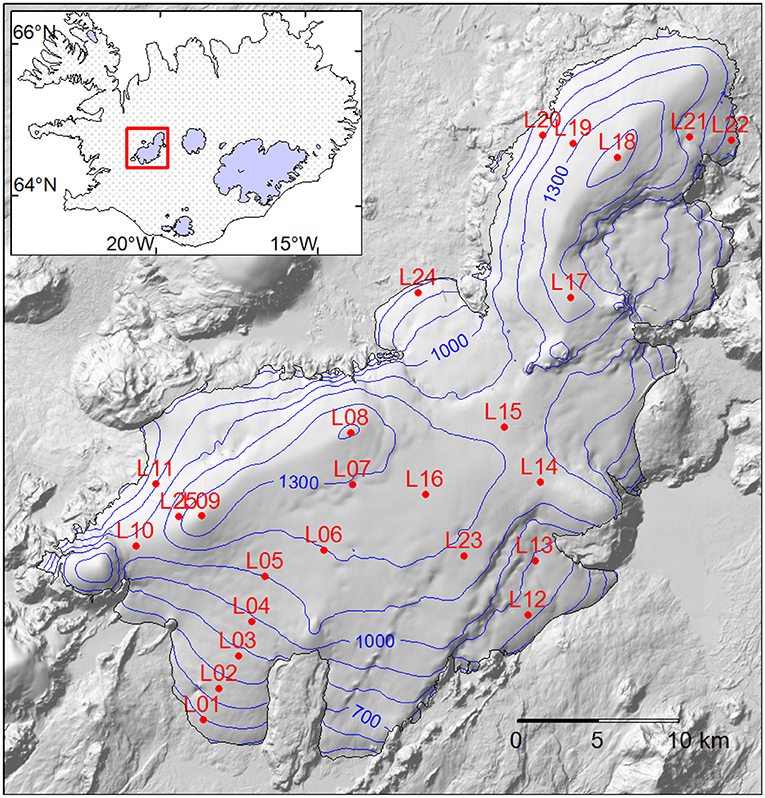
Figure 1. Surface topographical map of Langjökull along with surface velocity survey locations.

Notice that the x and y velocity equations given in Equations (2.1) and (2.2) require glacial thickness and the surface elevation derivatives with respect to x and y. The former is obtained with the difference between surface elevation and bed elevation, and the latter is obtained with central differences of the surface elevation topographical maps. The Langjökull surface elevation ranges from 440 to 1,440 m above sea level. The grid that contains the surface elevation data and bed measurements is of dimensions 43,800 m by 46,400 m. Langjökull is about 50 km long and 20 km wide, which explains the name “long glacier.”

3. Results

The posterior mean of ice softness using the t distribution is 18.2 with a posterior standard deviation of 0.847, and the posterior mean for ice softness using the normal distribution is 17.8 with a posterior standard deviation of 1.11 (units of 10⁻²⁵s⁻¹Pa⁻³). For comparison, 23.7 is estimated by Gudmundsson (1999), 23.4 is found in Aðalgeirsdóttir et al. (2000), 22.2 is found in Albrecht et al. (2000), and 20 is found in Hubbard et al. (1998), also in units of 10⁻²⁵s⁻¹Pa⁻³. The recommended value from Cuffey and Paterson (2010) is 24 × 10⁻²⁵s⁻¹Pa⁻³. The posterior distributions for ice softness appears to be in the vicinity of these values, though strictly less. Using the t distribution for surface velocities, the posterior distribution for ice softness is slightly closer to the recommended value for temperate glaciers from Cuffey and Paterson (2010) than when the normal distribution is used, and has a lower standard deviation (i.e., more precise) as is illustrated in Figure 2. Moreover, plots of posterior means for x and y velocities vs. observed x and y velocities are displayed in Figure 3 and show a generally close agreement; the few outliers in the x velocity direction are at locations close to the outer edge of the glacier where the SIA is a poorer physical description. As velocities are dependent on both ice viscosity and basal sliding, the overall agreement between observed and predicted surface velocities indicates that inferences are physically realistic.

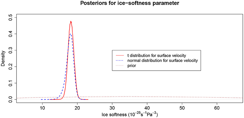
Figure 2. Illustration of posterior densities for ice softness using a normal distribution and t distribution for surface velocities. The prior, nearly flat, is also shown for comparison. Units are 10⁻²⁵s⁻¹Pa⁻³.

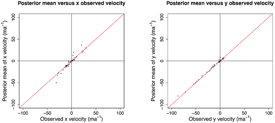
Figure 3. An illustration of the posterior mean for x and y glacier surface velocities compared to the observed x and y glacier surface velocities (using a t distribution for surface velocities). Units for velocities are in meters per year. Overall, the observed and inferred values agree, particularly for the y-velocity values.

An important consequence of the model output is the ability to decompose posterior ice velocity into a ice deformation component (referred to as viscous flow in Minchew et al., 2015) and a sliding component. The panels of Figure 4 map the posterior mean of deformation velocities and sliding velocities across Langjökull during the melt seasons of 2007 and 2015, and are overlaid on surface elevation topography. Several important observations are apparent based on these maps. First is that the direction of velocity in the negative of the surface gradient, evident based on the directions pointing toward areas of rapid elevation descent. The second main observation is that there are two important regions of significant basal sliding in the southwest and north of the glacier. In the southwest (i.e., W-Hagafellsjökull) the bed consists of gentle slopes of layers of lava flows of a shield volcano (now even visible at the glacier edge), and in the north region hard bed is also likely, whereas much of Langjökull bed is probably of more permeable bedrock or sediments. Less permeability makes it more likely for meltwater to heighten the water pressure at the bed, at the start of melting periods (which may occur more than once during the melt season), thus creating conditions for basal sliding.

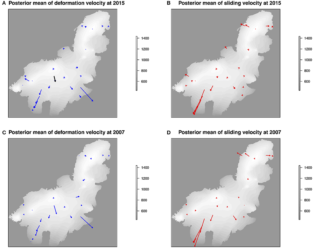
Figure 4. Illustration of posterior mean horizontal surface velocities across Langjökull during the 2007 and 2015 melt seasons. (A,B) illustrate 2015 velocities due to deformation (i.e., viscous flow) and sliding, respectively. (C,D) illustrate 2007 velocities due to deformation (i.e., viscous flow) and sliding, respectively. The velocities are overlaid on surface topographical maps (elevation in meters), and the arrow directions are that of the steepest descent. The lengths of the arrows are proportional to speed: the black arrow on panel (A) corresponds to 12.4 m/a. Substantial sliding appears to occur in the southwest and north; the sliding magnitude appears to be slightly less in 2015 compared to 2007, which corresponds to about 1/3 less melt during 2015 based on mass balance measurements.

In Minchew et al. (2015) Figures 4C,D, maps of speed assuming only viscous (i.e., deformational flow) are compared to maps of measured speeds with InSAR at Langjökull; the difference between the two is indicative of the amount that basal sliding contributes to surface velocity. These maps also show evidence of significant basal sliding velocity in the north and southwest of Langjökull, consistent with the spatial variation we have observed in posterior basal sliding speeds. Additionally, we see a significant posterior deformation velocity component in the southeastern part of Langjökull (see the arrow that runs off of the body of Langjökull in the southeast), where basal sliding is quite low. This result is also consistent with Minchew et al. (2015) because deformation speed is quite close to total speed in this region (Figures 4C,D of Minchew et al., 2015). We do not notice significant temporal variation in posterior velocities except for what appears to be a slight reduction in basal sliding velocities in the north and southwest regions. This finding is likely to be related to less summer melt (about a third) in summer 2015 than in 2007 observed via mass balance measurements.

In addition to maps of posterior basal sliding and deformation, Section 5 Figures A7–A10 provide illustrations of the posterior uncertainty in the basal sliding parameter for 2007 and 2015. The numbers on the maps indicate the measurement sites, and the boxplots that follow have numbering on the horizontal axis corresponds to the numbering on the map. The boxplots plot the posterior distribution for the basal sliding parameter at the corresponding site, illustrating the uncertainty in the posterior distribution. The regions that show large amounts of basal sliding, both in 2007 and 2015, are in areas with large basal sliding speeds, as illustrated in Figure 4; these regions are in the southwest and north. Moreover, uncertainty in basal sliding is much larger in the north than in the southwest, both in 2007 and 2015. In the southwest, the basal sliding parameters appear to be larger in 2007 than in 2015 (just under 4 × 10⁻⁴ in 2007 vs. 3 × 10⁻⁴ in 2015 in units of ma⁻¹Pa⁻¹). The reduced amount of basal sliding corresponds to about a 1/3 reduction in melt as measured by mass balance measurements in 2015 and 2007.

4. Discussion

The objective of this paper is to develop Bayesian models for glacier surface velocity, based on a shallow ice approximation, that allow for the statistical inference of important glacial parameters: ice softness and basal sliding. Specifically, one model stipulates a normal distribution for surface velocities, whereas the other specifies a heavy-tailed t distribution.

Overall, a notable result is that the posterior distribution for ice softness is close to values derived in the literature (for instance, the recommended value from Cuffey and Paterson, 2010), albeit by different methods. In contrast to these works, the estimate of ice softness is accompanied with an uncertainty estimate as well via the posterior standard deviation. An additional differentiating aspect of our work in comparison to other Bayesian approaches involving glacial surface velocity is the use of a t distribution in addition to a normal distribution (an assumption used in Pralong and Gudmundsson, 2011; Brinkerhoff et al., 2016 to give a few examples). The pattern of spatial variation in basal sliding is also consistent with prior studies of surface velocity at Langjökull, in particular Minchew et al. (2015). However, it is important to note that these patterns of spatial variation in basal sliding are specifically during the melt season, so it is not possible to verify how the approach performs for inferring sliding velocities during the winter-spring season when the total velocity is expected to be almost due to deformation only.

The residual analysis detailed in the Appendix (section 5) provides a means of assessing the normal distribution and t distribution used for surface velocities. Residuals are defined as centered and scaled versions of the x and y observed surface velocities (i.e., subtracting off the posterior mean of surface velocity and dividing by the posterior mean of the scale parameter for both directions). A Shapiro-Wilk test is conducted for the residuals, and the assumption of normality is rejected for both the x and y surface velocity residuals, providing evidence against the use of the normal distribution for surface velocities. Additionally, Figure A11 of section 5 provides quantile-quantile (QQ) plots comparing the sample quantiles with theoretical quantiles for the residuals assuming that a normal distribution holds. A good fit occurs when there is close agreement between sample and theoretical quantiles but is not observed for the normal distribution residuals, particularly for the x-velocity components. We also include a QQ-plot for the t distribution residuals in the second row of Figure A11. There is some improvement in the QQ-plot for the t distribution residuals of x-velocities, but not as much for the y-velocities, it appears. Overall the residual analysis supports the claim that a normal distribution is not a good fit for surface velocities and a heavy-tailed t distribution improves goodness-of-fit.

We must also lay forth limitations of our approach. Perhaps the greatest limitation is the use of the shallow ice approximation, which will not always hold. Another issue is that of scalability; the Gibbs sampler for posterior inference takes on the order of a few hours on 2020 iMac with 3.8 GHz 8-Core Intel Core i7 processor with a data set of 51 surface velocity observations. The approach may be more time consuming with a larger data set, especially for the Gaussian process prior for basal sliding parameters, whose probability density involves finding the inverse and determinant of a covariance matrix, generally computationally costly operations.

There are a number of future steps that can be taken to extend this analysis. First, the posterior distributions for the physical parameters can be used in Monte Carlo simulations involving a time dynamical model of glacier evolution in order to derive projections for how the shape of Langjökull will evolve in the future. Second, alternate continuous distributions may be tested besides the normal or t distribution used within this work (perhaps even a non-parametric distribution). Third, additional correlation structures besides the Matérn kernel can be investigated for the prior distribution on the basal sliding field.

While the models have been exclusively applied to Langjökull, we believe this work serves as a guide for selecting physical parameters and quantifying their uncertainty at other temperate, shallow glaciers around the globe, the melting of which is expected to contribute significantly to sea level rise in the next century. Additonally, the R code written for performing Bayesian inference with a Gibbs sampler may be reapplied for other scenarios where surface topography, bed topography, and surface velocity data are available. Despite that the models we have used rely on a SIA, different equations for v_x and v_y, for instance based on a numerical solver, may be used.

Data Availability Statement

The original contributions presented in the study are included in the article/Supplementary Material, further inquiries can be directed to the corresponding author/s.

Author Contributions

GG developed the model, completed programming, and wrote the manuscript. Additional authors provided valuable feedback, guidance, and manuscript help. FP provided glacier data for conducting analysis. All authors contributed to the article and approved the submitted version.

Funding

This work is from the lead author's Ph.D. work with the University of Iceland. The work was funded by the Icelandic Research Fund (RANNIS) by a grant entitled: Statistical Models for Glaciology. Grant number was 152457-051.

Conflict of Interest

The authors declare that the research was conducted in the absence of any commercial or financial relationships that could be construed as a potential conflict of interest.

The reviewer GF declared a past co-authorship with several of the authors GA and FP to the handling editor.

Supplementary Material

The Supplementary Material for this article can be found online at: https://www.frontiersin.org/articles/10.3389/feart.2021.610069/full#supplementary-material

References

Aðalgeirsdóttir, G., Gudmundsson, G. H., and Björnsson, H. (2000). The response of a glacier to a surface disturbance: a case study on Vatnajökull ice cap, Iceland. Ann. Glaciol. 31, 104–110. doi: 10.3189/172756400781819914
Albrecht, O., Jansson, P., and Blatter, H. (2000). Modelling glacier response to measured mass-balance forcing. Ann. Glaciol. 31, 91–96. doi: 10.3189/172756400781819996
Bakka, H., Rue, H., Fuglstad, G.-A., Riebler, A., Bolin, D., Illian, J., et al. (2018). Spatial modeling with R-INLA: a review. Wiley Interdiscipl. Rev. Comput. Stat. 10:e1443. doi: 10.1002/wics.1443
Björnsson, H. (2017). The Glaciers of Iceland: A Historical, Cultural and Scientific Overview. Springer. Available online at: https://www.springer.com/gp/book/9789462392069
Björnsson, H., Aðalgeirsdóttir, G., Guðmundsson, S., Jóhannesson, T., Pálsson, F., and Sigurðsson, O. (2006). “Climate change response of vatnajökull, hofsjökull and Langjökull ice caps, iceland,” in European Conference on Impacts of Climate Change on Renewable Energy Sources (Reykjavik).
Björnsson, H., and Pálsson, F. (2020). Radio-echo soundings on Icelandic temperate glaciers: history of techniques and findings. Ann. Glaciol. 61, 25–34. doi: 10.1017/aog.2020.10
Björnsson, H., Pálsson, F., Sigurđsson, O., and Flowers, G. E. (2003). Surges of glaciers in iceland. Ann. Glaciol. 36, 82–90. doi: 10.3189/172756403781816365
Brinkerhoff, D. J., Aschwanden, A., and Truffer, M. (2016). Bayesian inference of subglacial topography using mass conservation. Front. Earth Sci. 4:8. doi: 10.3389/feart.2016.00008
Bueler, E., Lingle, C. S., Kallen-Brown, J. A., Covey, D. N., and Bowman, L. N. (2005). Exact solutions and verification of numerical models for isothermal ice sheets. J. Glaciol. 51, 291–306. doi: 10.3189/172756505781829449
Cuffey, K. M., and Paterson, W. (2010). The Physics of Glaciers, 4 Edn. Oxford, UK: Academic Press. Available online at: https://www.elsevier.com/books/the-physics-of-glaciers/cuffey/978-0-12-369461-4
Flowers, G. E., Björnsson, H., Geirsdóttir, Á., Miller, G. H., and Clarke, G. K. (2007). Glacier fluctuation and inferred climatology of Langjökull ice cap through the little ice age. Q. Sci. Rev. 26, 2337–2353. doi: 10.1016/j.quascirev.2007.07.016
Gelfand, A. E., Diggle, P., Guttorp, P., and Fuentes, M. (2010). Handbook of Spatial Statistics. Boca Raton, FL: CRC Press.
Gelman, A., and Rubin, D. B. (1992). Inference from iterative simulation using multiple sequences. Statist. Sci. 7, 457–472.
Gopalan, G., Hrafnkelsson, B., Aðalgeirsdóttir, G., Jarosch, A. H., and Pálsson, F. (2018). A Bayesian hierarchical model for glacial dynamics based on the shallow ice approximation and its evaluation using analytical solutions. Cryosphere 12, 2229–2248. doi: 10.5194/tc-12-2229-2018
Guan, Y., Haran, M., and Pollard, D. (2016). Inferring ice thickness from a glacier dynamics model and multiple surface datasets. ArXiv pre-prints. doi: 10.1002/env.2460
Gudmundsson, G. H. (1999). A three-dimensional numerical model of the confluence area of unteraargletscher, bernese alps, Switzerland. J. Glaciol. 45, 219–230.
Hock, R., Rasul, G., Adler, C., Cáceres, B., Gruber, S., Hirabayashi, Y., et al. (2019). “High mountain areas,” in Ipcc Special Report on the Ocean and Cryosphere in a Changing Climate. Available online at: https://www.ipcc.ch/srocc/chapter/chapter-2/.
Hubbard, A., Blatter, H., Nienow, P., Mair, D., and Hubbard, B. (1998). Comparison of a three-dimensional model for glacier flow with field data from haut glacier d'arolla, Switzerland. J. Glaciol. 44, 368–378. doi: 10.1017/S0022143000002690
Hutter, K. (1983). Theoretical Glaciology: Material Science of Ice and the Mechanics of Glaciers and Ice Sheets. Mathematical Approaches to Geophysics. Heidelberg: Springer.
Isaac, T., Petra, N., Stadler, G., and Ghattas, O. (2015). Scalable and efficient algorithms for the propagation of uncertainty from data through inference to prediction for large-scale problems, with application to flow of the antarctic ice sheet. J. Comput. Phys. 296, 348–368. doi: 10.1016/j.jcp.2015.04.047
Jarosch, A. H., Schoof, C. G., and Anslow, F. S. (2013). Restoring mass conservation to shallow ice flow models over complex terrain. Cryosphere 7, 229–240. doi: 10.5194/tc-7-229-2013
Marshall, S. J., Björnsson, H., Flowers, G. E., and Clarke, G. K. C. (2005). Simulation of Vatnajökull ice cap dynamics. J. Geophys. Res. Earth Surf. 110. doi: 10.1029/2004JF000262
Minchew, B., Simons, M., Hensley, S., Björnsson, H., and Pálsson, F. (2015). Early melt season velocity fields of Langjökull and Hofsjökull, central Iceland. J. Glaciol. 61, 253–266. doi: 10.3189/2015JoG14J023
Murray, I., Adams, R. P., and MacKay, D. J. (2010). Elliptical slice sampling. J. Mach. Learn. Res. 9, 541–548.
Pálsson, F., Guðmundsson, S., Björnsson, H., Berthier, E., Magnússon, E., Guðmundsson, S., et al. (2012). Mass and volume changes of Langjökull ice cap, iceland, 1890 to 2009, deduced from old maps, satellite images and in situ mass balance measurements. Jökull 62, 81–96.
Petra, N., Martin, J., Stadler, G., and Ghattas, O. (2014). A computational framework for infinite-dimensional bayesian inverse problems, part II: stochastic newton mcmc with application to ice sheet flow inverse problems. SIAM J. Sci. Comput. 36, A1525–A1555. doi: 10.1137/130934805
Pope, E. L., Willis, I. C., Pope, A., Miles, E. S., Arnold, N. S., and Rees, W. G. (2016). Contrasting snow and ice albedos derived from modis, landsat etm+ and airborne data from Langjökull, iceland. Remote Sens. Environ. 175, 183–195. doi: 10.1016/j.rse.2015.12.051
Porter, C., Morin, P., Howat, I., Noh, M.-J., Bates, B., Peterman, K., et al. (2018). ArcticDEM. doi: 10.7910/DVN/OHHUKH. Harvard Dataverse, V1.
Pralong, M. R., and Gudmundsson, G. H. (2011). Bayesian estimation of basal conditions on Rutford Ice Stream, West Antarctica, from surface data. J. Glaciol. 57, 315–324. doi: 10.3189/002214311796406004
Raymond, M. J., and Gudmundsson, G. H. (2009). Estimating basal properties of ice streams from surface measurements: a non-linear bayesian inverse approach applied to synthetic data. Cryosphere 3, 265–278. doi: 10.5194/tc-3-265-2009
Tierney, L. (1994). Markov chains for exploring posterior distributions. Ann. Statist. 22, 1701–1728.
Vats, D., and Knudson, C. (2018). Revisiting the Gelman-Rubin diagnostic. arXiv preprint arXiv:1812.09384.
Werder, M. A., Huss, M., Paul, F., Dehecq, A., and Farinotti, D. (2020). A Bayesian ice thickness estimation model for large-scale applications. J. Glaciol. 66, 137–152. doi: 10.1017/jog.2019.93
Keywords: surface velocity, basal sliding, data analysis-methods, Bayesian inference, ice properties
Citation: Gopalan G, Hrafnkelsson B, Aðalgeirsdóttir G and Pálsson F (2021) Bayesian Inference of Ice Softness and Basal Sliding Parameters at Langjökull. Front. Earth Sci. 9:610069. doi: 10.3389/feart.2021.610069
Received: 24 September 2020; Accepted: 12 April 2021;
Published: 10 May 2021.
Edited by:
Alun Hubbard, Aberystwyth University, United KingdomReviewed by:
Douglas John Brinkerhoff, University of Montana, United StatesGwenn Flowers, Simon Fraser University, Canada
Copyright © 2021 Gopalan, Hrafnkelsson, Aðalgeirsdóttir and Pálsson. This is an open-access article distributed under the terms of the Creative Commons Attribution License (CC BY). The use, distribution or reproduction in other forums is permitted, provided the original author(s) and the copyright owner(s) are credited and that the original publication in this journal is cited, in accordance with accepted academic practice. No use, distribution or reproduction is permitted which does not comply with these terms.
*Correspondence: Giri Gopalan, ggopalan@calpoly.edu