A Self-Supervised Deep Learning Reconstruction for Shortening the Breathhold and Acquisition Window in Cardiac Magnetic Resonance Fingerprinting
 Jesse I. Hamilton
- 1Department of Radiology, University of Michigan, Ann Arbor, MI, United States
- 2Department of Biomedical Engineering, University of Michigan, Ann Arbor, MI, United States
The aim of this study is to shorten the breathhold and diastolic acquisition window in cardiac magnetic resonance fingerprinting (MRF) for simultaneous T1, T2, and proton spin density (M0) mapping to improve scan efficiency and reduce motion artifacts. To this end, a novel reconstruction was developed that combines low-rank subspace modeling with a deep image prior, termed DIP-MRF. A system of neural networks is used to generate spatial basis images and quantitative tissue property maps, with training performed using only the undersampled k-space measurements from the current scan. This approach avoids difficulties with obtaining in vivo MRF training data, as training is performed de novo for each acquisition. Calculation of the forward model during training is accelerated by using GRAPPA operator gridding to shift spiral k-space data to Cartesian grid points, and by using a neural network to rapidly generate fingerprints in place of a Bloch equation simulation. DIP-MRF was evaluated in simulations and at 1.5 T in a standardized phantom, 18 healthy subjects, and 10 patients with suspected cardiomyopathy. In addition to conventional mapping, two cardiac MRF sequences were acquired, one with a 15-heartbeat(HB) breathhold and 254 ms acquisition window, and one with a 5HB breathhold and 150 ms acquisition window. In simulations, DIP-MRF yielded decreased nRMSE compared to dictionary matching and a sparse and locally low rank (SLLR-MRF) reconstruction. Strong correlation (R2 > 0.999) with T1 and T2 reference values was observed in the phantom using the 5HB/150 ms scan with DIP-MRF. DIP-MRF provided better suppression of noise and aliasing artifacts in vivo, especially for the 5HB/150 ms scan, and lower intersubject and intrasubject variability compared to dictionary matching and SLLR-MRF. Furthermore, it yielded a better agreement between myocardial T1 and T2 from 15HB/254 ms and 5HB/150 ms MRF scans, with a bias of −9 ms for T1 and 2 ms for T2. In summary, this study introduces an extension of the deep image prior framework for cardiac MRF tissue property mapping, which does not require pre-training with in vivo scans, and has the potential to reduce motion artifacts by enabling a shortened breathhold and acquisition window.
Introduction
Cardiac magnetic resonance (CMR) T1 and T2 mapping are useful for the detection of pathological changes in myocardial tissue, including acute (1) and chronic inflammation (2, 3), edema (4, 5), amyloid deposition (6), fatty infiltration (7), and infarct (8). Multiparametric methods have recently been developed to efficiently measure multiple tissue properties during one scan (9–12). Cardiac magnetic resonance fingerprinting (MRF) is one such technique that uses a time-varying pulse sequence to encode several properties in magnetization signal evolutions over time (13, 14). A time series of highly undersampled images is acquired, typically with a single image frame collected per repetition time (TR). Quantitative maps are obtained using pattern recognition, where the signal evolution (or “fingerprint”) measured at each voxel is matched to a dictionary of fingerprints simulated for different tissue property values.
While simultaneous T1, T2, and proton spin density (M0) mapping using cardiac MRF has been demonstrated in healthy subjects (15) and cardiomyopathy patients (16), respiratory and cardiac motion present significant challenges, even when breathholding and electrocardiogram (ECG) triggering are employed. The highly accelerated non-Cartesian sampling used in cardiac MRF introduces noise-like artifacts in the measured fingerprints, and thus many image frames are collected to enable accurate pattern recognition using the corrupted signals. Several previous studies employed a relatively long breathhold of 15 heartbeats and diastolic acquisition window of approximately 250 ms as a result (15). However, this sequence may be susceptible to motion if patients have difficulty holding their breath or have elevated heart rates. While retrospective motion correction can be used (17), an alternative strategy is to shorten the breathhold and acquisition window to avoid the need for such corrections.
Shortening the MRF acquisition will result in fewer time points in each fingerprint, which can impede accurate pattern recognition. Several classes of reconstruction methods have been developed to accelerate MRF scans, including model-based reconstructions (18, 19), low-rank subspace techniques (20–22), and deep learning (23). Deep learning methods have gained particular interest for their excellent denoising capabilities and fast computation times. While some MRF deep learning reconstructions operate on single-voxel fingerprints (23, 24), others use the fingerprints from many voxels within a spatial neighborhood to estimate the tissue properties at a target voxel (25), and thus can leverage both spatial and temporal correlations in the MRF data to reduce noise and k-space undersampling artifacts. Such a method was recently demonstrated for MRF in the brain, where a convolutional neural network (CNN) reconstruction enabled a 4-fold reduction in scan time compared to conventional dictionary matching (25) and allowed for high-resolution (submillimeter) mapping (26).
However, CNN reconstructions typically require training using in vivo datasets, which presents a challenge for cardiac MRF. It is difficult to collect ground truth tissue property maps in the heart due physiological motion, as a scan time of several minutes would be needed to obtain fully-sampled MRF data. Furthermore, because the MRF scan is prospectively triggered, the fingerprints depend on the subject’s cardiac rhythm (14), and thus many datasets from subjects with different cardiac rhythms (including fast or irregular rhythms commonly seen in patients) would potentially be needed for training.
Recently, a deep image prior (DIP) technique was proposed for image processing tasks that does not require pre-training with ground truth datasets (27). Taking image denoising as an example, a randomly initialized CNN learns to generate a denoised image by minimizing the mean squared error loss compared to a noise-corrupted image, with no requirements for additional training data. The network architecture is typically based on a u-net (28) and is designed so that lower spatial frequencies are recovered before higher spatial frequencies (29). Therefore, the network learns to generate natural images before recovering higher frequency noise, so that training with early stopping avoids overfitting to the noisy image. When applied to inverse problems in medical imaging, a mathematical model of the image acquisition can be incorporated in the loss function, which has been applied to computed tomography (30), positron emission tomography (31), and diffusion MRI (32).
This study introduces a self-supervised deep learning reconstruction for cardiac MRF T1, T2, and M0 mapping for the purpose of mitigating noise, reducing k-space undersampling artifacts, and enabling a shortened acquisition to reduce motion artifacts. The proposed method, termed DIP-MRF, combines low-rank MRF subspace modeling with the denoising capabilities of a deep image prior. A system of convolutional (u-net) and fully-connected networks is used to generate spatial basis images (i.e., images in a low-dimensional subspace derived from the MRF signal evolutions) and quantitative maps, without dictionary matching and without pre-training using in vivo data. For each MRF acquisition, training is performed de novo using only the undersampled k-space measurements from the current scan by incorporating a mathematical model of the cardiac MRF data acquisition in the loss function. DIP-MRF is shown to reduce noise and undersampling artifacts compared to conventional dictionary matching and low-rank subspace reconstructions. Furthermore, DIP-MRF is leveraged to shorten the breathhold duration from 15 to 5 heartbeats and diastolic acquisition window from 250 to 150 ms, with results shown in healthy subjects and cardiomyopathy patients, which has the potential to reduce motion artifacts.
Materials and Methods
Previous work has shown that an MRF dictionary, denoted by D ∈ ℂp×t, where p is the number of parameter combinations and t is the number of time points, can be compressed along time using a truncated singular value decomposition (SVD) that retains only the first k singular values (33). The temporal basis functions are denoted by Vk ∈ ℂt×k, which is matrix whose columns contain the first k right singular vectors. A compressed dictionary, denoted by Dk ∈ ℂp×k, can be obtained according to Dk=DVk. Similarly, if x ∈ ℂn×t denotes a time series of MRF images with n voxels, then multiplication by V_k yields a set of spatial basis images in this low-dimensional subspace, denoted by xk=xVk, where xk ∈ ℂn×k. Multiplying the spatial basis images by the complex conjugate will yield a low-rank approximation to the original MRF image series, . Low-rank subspace reconstructions for MRF have been proposed that iteratively remove noise and undersampling artifacts from the spatial basis images, sometimes with additional regularization terms using spatial sparsity and/or locally low rank regularization, before matching to the compressed dictionary to obtain quantitative maps (21, 22, 34, 35).
This study extends the deep image prior framework using a low-rank cardiac MRF signal model. An overview of the DIP-MRF reconstruction pipeline is shown in Figure 1. A convolutional u-net generates spatial basis images, which are input to a fully-connected network that outputs quantitative maps, neither of which require pre-training with in vivo data. Rather, the networks are trained in a self-supervised manner to enforce consistency with the undersampled k-space data from a single scan by incorporating the MRF forward encoding model in the loss function. The forward model includes (1) simulation of a time series of MRF images from the tissue property maps, (2) projection of images onto the low-dimensional subspace, (3) coil sensitivity encoding, and (4) spiral k-space undersampling. Calculation of the forward model is accelerated by (1) a pre-trained neural network that rapidly outputs fingerprints instead of using a more time-consuming Bloch equation simulation (36), and (2) preprocessing the spiral MRF k-space data with GRAPPA operator gridding (GROG) to obtain data in Cartesian k-space (37). The following sections will describe the DIP-MRF pipeline in more detail.
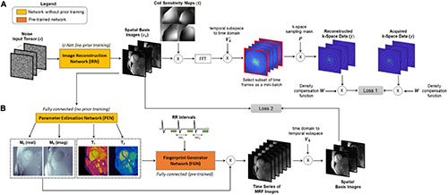
Figure 1. Overview of the DIP-MRF reconstruction. A system of neural networks outputs spatial basis images and T1, T2, and M0 maps, with no additional in vivo training data needed beyond the undersampled k-space data from the current scan. (A) The image reconstruction network (IRN) is a convolutional u-net that outputs a set of k spatial basis images. The input is a tensor of random numbers that remains fixed throughout training. Training is performed in a self-supervised manner by simulating the cardiac MRF forward encoding model. This step includes multiplication by coil sensitivity maps, fast Fourier transformation (FFT), projection of k-space data from the low-dimensional subspace to the time domain, and multiplication by spiral undersampling masks. The resulting k-space data are compared to the acquired k-space measurements, after density compensation, at the sampled locations using a mean squared error loss function (Loss 1), and IRN is updated using backpropagation. (B) A fully-connected network, referred to as the Parameter Estimation Network (PEN), uses the spatial basis images to output tissue property maps. Specifically, it outputs T1, T2, and a complex-valued M0 scaling term. The T1 map, T2 map, and cardiac rhythm timings (RR intervals) from the ECG are input to the fingerprint generator network, which is a pre-trained fully-connected network that can be thought of as an efficient Bloch equation simulator that rapidly outputs cardiac MRF signal evolutions (fingerprints). The simulated fingerprints at all voxels are multiplied by the complex M0 map to yield a time series of images. The images are projected onto the low-dimensional subspace and compared to the spatial basis images that were output by the IRN using a mean squared error loss function, and the PEN is updated using backpropagation (Loss 2). Note that the IRN and PEN are trained in parallel.
Pre-trained Fingerprint Generator Network
Calculating the forward model requires repeated simulations of MRF signal evolutions at every iteration. To reduce computation time, this step is performed using a neural network called the Fingerprint Generator Network (FGN), which rapidly outputs signal evolutions for arbitrary T1, T2, and cardiac rhythm timings (Figure 2A) and has been described previously (36). The network is fully-connected with two hidden layers and 300 nodes per layer. The input consists of a T1 value, a T2 value, and the subject’s cardiac rhythm timings (specifically, a vector of RR interval times) recorded by the ECG during the scan. The output is a vector of length 2t containing interleaved real and imaginary parts of the fingerprint. The FGN is the only neural network component in the DIP-MRF pipeline that requires pre-training. The pre-training is performed only one time using fingerprints produced by a Bloch equation simulation for different T1, T2, and cardiac rhythm timings, after which the same network can be applied to any subsequent scan regardless of the subject’s cardiac rhythm. Supplementary Figure 1 gives additional details about pre-training the FGN.
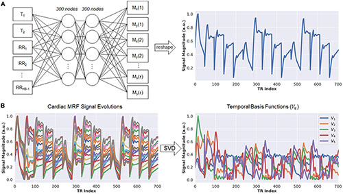
Figure 2. Schematic of the fingerprint generator network (FGN) and derivation of the low-dimensional subspace. (A) The FGN is a fully-connected network with two hidden layers. The input consists of a T1 value, T2 value, and vector of RR interval times (RR1, RR2, …, RRHB–1) recorded by the ECG, where RRi denotes the elapsed time (in milliseconds) between the end of the acquisition window in heartbeat i and the beginning of the acquisition window in heartbeat i+1, and HB is the total number of heartbeats in the scan. The output is a vector of length 2t, where t is the number of repetition times (i.e., number of time points), which contains the interleaved real and imaginary parts of an MRF fingerprint. (B) The FGN is used to calculate a dictionary of fingerprints for different T1 and T2 combinations specific for the patient’s cardiac rhythm timings (left panel). The SVD of the dictionary is calculated in order to derive the low-rank approximation used in the DIP-MRF forward model calculation (right panel).
Low-Rank Signal Approximation
Although DIP-MRF does not use pattern recognition, a dictionary of fingerprints is calculated temporarily in order to derive the temporal basis functions V_k (33). The FGN is used to output a dictionary of approximately 23,000 fingerprints with T1 between 50–3,000 ms and T2 between 5–1,000 ms, which takes 30 ms on a GPU. Next, the SVD of the dictionary is calculated (taking approximately 1 s), and the temporal basis functions are obtained from the first k right singular vectors (Figure 2B). This study uses a rank of k = 5, which retains more than 99.9% of the energy compared to the uncompressed fingerprints.
GRAPPA Operator Gridding Preprocessing and Coil Sensitivity Estimation
The forward model calculation requires repeated iterations between image and k-space domains. To avoid time-consuming operations using the non-uniform fast Fourier Transform (NUFFT) (38), the MRF spiral k-space data are preprocessed using GROG, a parallel imaging technique that shifts non-Cartesian k-space data to unmeasured Cartesian locations using GRAPPA weight matrices (37). The weight matrices for unit shifts along k_x and k_y are calibrated using a fully-sampled dataset; this dataset is obtained by taking the temporal average of the multicoil MRF k-space data, gridding a time-averaged image using the NUFFT, and performing an FFT to obtain multicoil Cartesian k-space data. The central 48 × 48 region of the Cartesian k-space is used for GROG calibration. Coil sensitivity maps are estimated from the time-averaged multicoil images using the adaptive combination method (39). The GROG density compensation function, denoted by W, is obtained by counting the number of spiral k-space points that are shifted to each Cartesian coordinate. After calibration, the GROG weights are applied to shift undersampled spiral MRF k-space data onto a Cartesian grid, and each time frame of the resulting Cartesian k-space dataset is multiplied by W. A binary mask, denoted by P_i, is stored that indicates the sampled (acquired) points on the Cartesian grid at each time index i.
Neural Network Architectures
A convolutional u-net, which is not pre-trained, is used to output the MRF spatial basis images. This network will be called the image reconstruction network (IRN) and is shown in Figure 3. Inspired by the original DIP publication (27), the input is a tensor denoted by z ∈ ℝny×nx×d of uniform random numbers between −0.1 and 0.1, where n_y and n_x are the spatial dimensions in voxels, and d is a tunable parameter defining the number of feature channels in the first layer of the network. This study uses d = 32 to be consistent with the original DIP work, but this parameter was not found to have much impact on the reconstruction. The IRN performs a series of 2D convolutions followed by batch normalization, leaky ReLU activation, and an optional dropout layer. The data pass through five downsampling and upsampling paths with multiple skip connections. Downsampling is implemented using convolution with a 2 × 2 stride, and upsampling is performed using nearest neighbor interpolation followed by convolution. The network output has size ny×nx×2k, where the channel dimension contains the interleaved real and imaginary parts of the k spatial basis images.
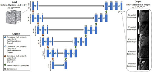
Figure 3. Schematic of the image reconstruction network (IRN), which outputs MRF spatial basis images. The input, z, is a tensor of uniformly distributed random numbers between −0.1 and 0.1 that remains fixed while training the network. The network is a u-net that performs a series of 2D convolutions. It has five downsampling and upsampling paths with multiple shortcut connections. The network outputs the MRF spatial basis images—i.e., images in a low-dimensional subspace of rank k that was derived from a dictionary of simulated signal evolutions, as described in Figure 2. The number of 2D filters is listed above each convolutional layer (indicated by the blue rectangles).
A fully-connected network, which also is not pre-trained, outputs quantitative T1, T2, and M0 maps from the spatial basis images. This network will be called the parameter estimation network (PEN) and is shown in Figure 4. The PEN has two hidden layers with 300 nodes per layer. Before being input to the network, the spatial basis images are vectorized to have size (nynx)×(2k), where the second (channel) dimension contains interleaved real and imaginary signal intensities. The network output has one channel for each tissue property. As in previous MRF studies (13, 14), M0 is modeled as a complex-valued scaling factor between the measured and simulated fingerprints, so the output has four channels for T1, T2, and the real and imaginary parts of M0.
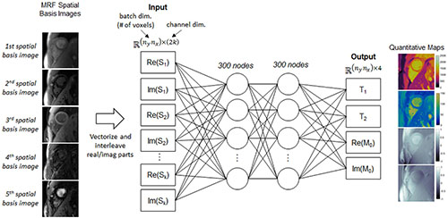
Figure 4. Schematic of the parameter estimation network (PEN), which estimates quantitative maps from the spatial basis images. Before being input to the network, the spatial basis images are first vectorized to have size n_yn_x (the batch dimension) by 2k (the channel dimension), where the channel dimension contains interleaved real and imaginary signal intensities from the k spatial basis images, and n_y and n_x are the spatial dimensions (number of voxels). The network has two hidden layers with 300 nodes per layer. The output has four channels corresponding to T1, T2, and the real and imaginary parts of the M0 scaling term.
Self-Supervised Training
The IRN and PEN networks are trained de novo for each reconstruction in a self-supervised manner (Figure 1). Both networks are initialized with random weights and biases. Additionally, the input (z) to the IRN is initialized with random numbers and remains fixed throughout training. Both networks are trained in parallel using a loss function with two terms, one for updating each network. First, letting θIRN denote the network parameters of the IRN, the spatial basis images generated by the IRN can be written as,
The spatial basis images are multiplied by coil sensitivity maps (S), transformed to k-space by performing an FFT, and multiplied by to yield time series data. To reduce memory requirements, a subset of time frames is selected as mini-batch at this point. In practice, this is implemented by using instead of V_k, where denotes the ith column vector from (note that multiplication by projects data from the subspace to the time domain and extracts only the ith time frame). The k-space data for time frame i are multiplied by the spiral undersampling mask for the corresponding time frame (P_i) and by the GROG density compensation function (W). The estimated multicoil k-space data for time frame i, denoted by , can be written as,
The first loss term is calculated as the mean squared error between and the acquired multicoil k-space measurements after density compensation, denoted by yi, at the sampled locations, and the IRN is updated using backpropagation.
The PEN is updated in parallel using a second loss term. The T1 and T2 maps output by the PEN, along with the subject’s RR interval times from the ECG, are input to the FGN to yield simulated fingerprints at each voxel location. These fingerprints are multiplied by the complex-valued M0 map to obtain a time series of images that are projected onto the subspace by multiplication with V_k. Letting θPEN and θFGN denote the network parameters of the PEN and FGN, respectively, the second loss term is calculated as the mean squared error between the resulting images and the spatial basis images output by the IRN:
For all experiments, training was performed for 30,000 iterations using an Adam optimizer with learning rate 0.001. DIP-MRF was implemented in Tensorflow (v2.8) with Keras on a GPU (NVIDIA Tesla v100 16GB). A mini-batch size of 32 image frames was used to calculate the loss for the IRN.
Cardiac Magnetic Resonance Fingerprinting Acquisition Parameters
Data were collected using a fast imaging with steady state precession (FISP) cardiac MRF sequence with a 15-heartbeat (HB) breathhold and 254 ms ECG-triggered diastolic acquisition (15, 40). Variable flip angles (4–25°) and a constant TR/TE of 5.4/1.4 ms were employed. A total of 705 undersampled images were collected (one image per TR) with 47 images acquired every heartbeat. Magnetization preparation pulses were applied before the acquisition window in each heartbeat according to the following schedule, which repeated three times during the scan: HB1—inversion (21 ms), HB2—no preparation, HB3—T2 prep (30 ms), HB4—T2 prep (50 ms), HB5—T2 prep (80 ms).
In addition, shortened MRF acquisitions were investigated having a five-heartbeat breathhold and progressively shorter acquisition windows. These were based on the same sequence structure, with the only difference being that the flip angle pattern within each heartbeat was truncated to fit within the desired scan window. An example of a flip angle series for a shortened scan is shown in Supplementary Figure 2. All data were acquired using a 48-fold undersampled spiral k-space trajectory (41) with a readout duration of 3.4 ms, matrix size of 192 × 192, field-of-view (FOV) of 300 × 300 mm2, and golden angle rotation of the trajectory every TR (42).
Simulation Experiments
Simulations were performed to investigate the feasibility of shortening the breathhold and diastolic scan window in cardiac MRF. In addition to the scan with a 15HB breathhold and 254 ms acquisition window (705 total TRs), scans with a 5HB breathhold and acquisition windows of 254 ms (235 total TRs), 200 ms (185 total TRs), 150 ms (140 total TRs), 100 ms (95 total TRs), and 50 ms (45 total TRs) were simulated. The MRF data acquisition was simulated, including Bloch equation signal simulation, coil sensitivity encoding with 8-channel sensitivity maps, and spiral k-space undersampling using the NUFFT. Complex Gaussian noise was added to the k-space data having a standard deviation of 0.1% of the maximum amplitude of the direct current (DC) signal. For each sequence variant, maps were reconstructed in three ways. In the first method (direct matching), one undersampled image was gridded every TR using the NUFFT, followed by dot product matching with a dictionary generated by a Bloch equation simulation to obtain T1, T2, and M0 maps (13). In the second method (SLLR-MRF), a sparse and locally low rank MRF reconstruction was performed (34), which yielded a set of k = 5 spatial basis images that were matched to an SVD-compressed dictionary. Locally low rank regularization with an 8 × 8 patch size and l_1-wavelet regularization were used with regularization weights of λLLR=0.02 and λwav=0.005 relative to the maximum intensity in the basis images. The reconstruction was solved using non-linear conjugate gradient descent with 25 iterations. The third method (DIP-MRF) consisted of GROG preprocessing followed by the DIP-MRF reconstruction. The reconstructions were compared using the normalized root mean square error (nRMSE) relative to the ground truth T1 and T2 maps, computed over all non-background voxels (i.e., all voxels where the ground truth M0 was non-zero).
A second set of simulations evaluated the robustness of DIP-MRF to noise. For the sequence with a 5HB breathhold and 150 ms acquisition window, complex Gaussian noise was added to the k-space data having standard deviations (σN) of 0, 0.1, 0.2, and 0.3% relative to the maximum amplitude of the DC signal. Maps were reconstructed using direct matching, SLLR-MRF, and DIP-MRF and compared in terms of nRMSE.
A third set of simulations assessed the impact of applying dropout during training (43). For the sequence with a 5HB breathhold and 150 ms acquisition window, the DIP-MRF reconstruction was repeated where different levels of dropout (0, 10, and 20%) were applied after each convolutional layer when training the IRN, and the maps were compared in terms of nRMSE.
Phantom Experiments
Experiments were performed using the ISMRM/NIST MRI system phantom (44) on a 1.5T scanner (MAGNETOM Sola, Siemens Healthineers, Erlangen, Germany). An 8 mm slice was planned through the T2 layer of the phantom, which has 14 spheres spanning a range of physiological relaxation times with T1 90–2,230 ms and T2 10–750 ms. An artificial heart rate of 60 bpm was simulated on the scanner. Data were collected using two cardiac MRF sequences: a sequence with a 15HB breathhold and 254 ms acquisition window and a sequence with a 5HB breathhold and 150 ms acquisition window. Maps were reconstructed using direct matching, SLLR-MRF, and DIP-MRF. Data were also acquired with conventional cardiac mapping sequences using Siemens MyoMaps software (45). T1 maps were collected with 5(3)3 modified look-locker inversion recovery (MOLLI) (46), and T2 maps were collected using a 1(3)1(3)1 T2-prepared balanced steady state free precession (bSSFP) sequence with T2 prep times of 0, 25, and 55 ms (5). Conventional cardiac mapping scans used GRAPPA with an acceleration factor of 2 and 24 autocalibration lines, 6/8 partial Fourier, a flip angle of 35°, and a scan window of 209 ms. All scans were collected with a matrix size of 192 × 192 and 300 mm2 FOV. Reference T1 values were measured using an inversion recovery spin echo sequence with TR = 10 s, TE = 12 ms, and inversion times of 21, 100, 200, 400, 800, and 1,600 ms. Reference T2 values were measured with a single-echo spin echo sequence with TR = 10 s and echo times of 10, 20, 40, 60, 100, 150, and 200 ms. Mean relaxation times were measured within each vial and compared to reference values using linear regression and Bland-Altman analyses (47). T2 values above 200 ms were excluded from analysis because the cardiac MRF sequence was not designed for that regime, considering that the longest T2 prep time was 80 ms (for completeness, measurements in all 14 vials are reported in the Supplementary Material).
Scans in Healthy Subjects and Patients
Eighteen healthy subjects were scanned at 1.5T after obtaining written informed consent in this IRB-approved, HIPAA-compliant study. All scans were performed during an end-expiratory breathhold at a mid-ventricular slice position. MOLLI and T2-prep bSSFP mapping were performed in all subjects. Data were also acquired using 15HB/254 ms and 5HB/150 ms cardiac MRF acquisitions, and maps were reconstructed using direct matching, SLLR-MRF, and DIP-MRF. To study the effects of training with dropout and to determine the optimal dropout percentage, the DIP-MRF reconstruction was repeated in three subjects with 0, 5, 10, 20, and 30% dropout applied after each convolutional layer when training the IRN. Unless otherwise states, the DIP-MRF reconstruction used dropout levels of 10 and 20% for the 15HB/254 ms and 5HB/150 ms MRF acquisitions, respectively.
In addition, data were collected in ten patients referred for a clinical CMR exam due to suspected cardiomyopathy. Native T1 and T2 maps were collected using the same protocol as in healthy subjects. Post-contrast T1 and T2 maps were acquired 15–25 min after IV injection of 0.2 mmol/kg body weight gadoteridol (ProHance, Bracco Diagnostics Inc., Princeton, NJ, United States). While post-contrast MRF scans (both 15HB/254 ms and 5HB/150 ms versions) were performed in all patients, post-contrast MOLLI and T2-prep bSSFP sequences were only collected in nine and three patients, respectively.
In vivo data were analyzed by manually segmenting the maps according to American Heart Association (AHA) guidelines (48). The mean and standard deviation for T1 and T2 were measured within each AHA segment and over all voxels in the myocardium. Similarly, T1 and T2 values were measured within the left (LV) and right ventricular (RV) blood pools after manual segmentation, taking care to avoid trabeculations and papillary muscles. Intersubject variability was quantified as the standard deviation of the mean T1 or T2 values over all subjects. Intrasubject variability was quantified by measuring the standard deviation in T1 or T2 for each subject and then calculating the mean over all subjects. T1 and T2 measurements using different reconstruction methods within the same subject were compared using a within-subjects ANOVA test with a Bonferroni post-hoc test for multiple comparisons, with p < 0.05 indicating statistical significance, as well as Bland-Altman plots. T1 and T2 measurements between healthy subjects and patients were compared using a two-sample t-test.
Results
Simulation Experiments
Figure 5A shows simulation results using MRF sequences with different breathhold and acquisition window lengths. In all cases, the nRMSE was highest with direct matching and lowest with DIP-MRF, and this difference was more pronounced for shorter sequence lengths. As the breathhold and acquisition window were shortened, nRMSE increased for direct matching and SLLR-MRF but remained consistently low for DIP-MRF. For the 15HB/254 ms sequence, the nRMSE was (T1 6.5%, T2 11.2%) for direct matching, (T1 2.9%, T2 4.3%) for SLLR-MRF, and (T1 1.4%, T2 0.7%) for DIP-MRF. For the 5HB/150 ms sequence, the nRMSE was (T1 13.4%, T2 20.2%) for direct matching, (T1 6.4%, T2 9.1%) for SLLR-MRF, and (T1 1.2%, T2 0.8%) for DIP-MRF. Supplementary Figure 3 shows examples of T1, T2, and M0 maps from the simulation study.
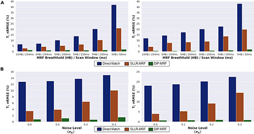
Figure 5. Simulation results in the MRXCAT phantom comparing the deep image prior (DIP-MRF) to direct matching and a low-rank subspace reconstruction (SLLR-MRF). (A) nRMSE plots of the T1 and T2 maps are shown for different cardiac MRF sequence lengths. Results are shown for MRF with a 15-heartbeat breathhold and 254 ms diastolic acquisition window, as well as shortened scans with a 5-heartbeat breathhold and successively shorter acquisition windows of 254, 200, 150, 100, and 50 ms. (B) nRMSE plots of the T1 and T2 maps are shown for the 5HB/150 ms MRF scan, where different amounts of random Gaussian noise having standard deviation σN (expressed as a percentage of the maximum DC signal level) were added to the simulated k-space data.
Figure 5B plots the nRMSE for the 5HB/150 ms sequence as the k-space data were corrupted with different amounts of complex Gaussian noise. The nRMSE was highest with direct matching and lowest with DIP-MRF at all noise levels. At the highest noise level tested (σN=0.3% of the DC signal), the nRMSE was (T1 14.9%, T2 22.5%) for direct matching, (T1 10.0%, T2 14.6%) for SLLR-MRF, and (T1 1.5%, T2 0.9%) for DIP-MRF.
Supplementary Figure 4 demonstrates the importance of applying dropout in DIP-MRF, with simulation results shown for the 5HB/150 ms sequence. Without dropout, the nRMSE reached a minimum (T1 1.7%, T2 1.0%) after approximately 5,000 iterations. The nRMSE increased gradually with further training due to overfitting to noise and undersampling artifacts, reaching (T1 2.2%, T2 1.4%) after 30,000 iterations. Using dropout improved the reconstruction accuracy, as the minimum nRMSE was lower compared to the 0% dropout case, and it reduced overfitting, allowing the network to be trained for longer without causing the nRMSE to increase. For example, with 20% dropout, the nRMSE reached a minimum of (T1 1.5%, T2 0.8%) after 12,000 iterations and only increased slightly to (T1 1.7%, T2 1.0%) after 30,000 iterations.
Phantom Experiments
Bland-Altman plots showing the agreement between 15HB/254 ms MRF, 5HB/150 ms MRF, and conventional mapping sequences relative to reference values are shown in Figure 6; linear regression plots of the same data are shown in Supplementary Figure 5, and T2 measurements in all 14 vials (including vials with T2 > 200 ms) are given in Supplementary Figures 6, 7. There were no significant differences in T1 or T2 relative to reference values for all MRF methods. Using DIP-MRF, the bias and 95% limits of agreement (LoA) for T1 were 4 ms (−45, 52)ms for the 15HB/254 ms sequence and −5 ms (−61, 51) ms for the 5HB/150 ms sequence; for T2, they were −0.9 ms (−5.5, 3.7) ms for the 15HB/254 ms sequence and 0.2 ms (−3.1, 3.4) ms for the 5HB/150 ms sequence. In general, DIP-MRF yielded narrower limits of agreement compared to direct matching and SLLR-MRF. MOLLI slightly underestimated T1 with a bias of −39 ms and 95% LoA of (−86, 8) ms. T2-prep bSSFP overestimated T2 with a bias of 35.6 ms and 95% LoA of (−45.9, 117.2) ms. This overestimation was larger for vials with short T2 values below approximately 100 ms, which is apparent on the linear regression plots (Supplementary Figure 5). The correlation coefficients were similar among all reconstructions for the 15HB/254 ms MRF sequence, with all R2> 0.998. For the 5HB/150 ms sequence, the correlation was slightly higher for DIP-MRF (R2= 0.999 for T1, R2= 1.000 for T2) compared to direct matching (R2= 0.998 for T1, R2= 0.995 for T2) and SLLR-MRF (R2= 0.998 for T1, R2= 0.999 for T2).
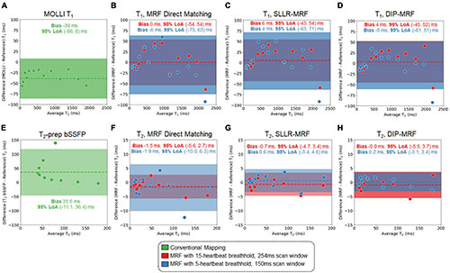
Figure 6. Bland-Altman plots from the phantom study. Plots are shown for T1 comparing (A) MOLLI and cardiac MRF with (B) direct matching, (C) SLLR-MRF, and (D) DIP-MRF reconstructions relative to gold standard measurements using an inversion recovery sequence. Similarly, plots are shown for T2 comparing (E) T2-prepared bSSFP and cardiac MRF with (F) direct matching, (G) SLLR-MRF, and (H) DIP-MRF reconstructions relative to gold standard measurements using a single-echo spin echo sequence. Results are shown for both 15HB/254 ms and 5HB/150 ms MRF sequences. The bias is indicated by a dotted line, and the 95% limits of agreement (LoA) are indicated by the solid colors.
Scans in Healthy Subjects
Representative maps in a healthy subject using 15HB/254 ms MRF, 5HB/150 ms MRF, and conventional mapping sequences are shown in Figure 7. Additional examples are provided in Supplementary Figures 8–10. Some noise enhancement was observed with direct matching for the 15HB/254 ms MRF sequence, with better map quality using SLLR-MRF and DIP-MRF reconstructions. The improvement using DIP-MRF was especially pronounced for the 5HB/150 ms sequence; direct matching led to severe noise enhancement and aliasing artifacts, SLLR-MRF provided only moderate noise suppression, and DIP-MRF gave the best suppression of noise and aliasing artifacts while preserving high resolution details, such as the papillary muscles.
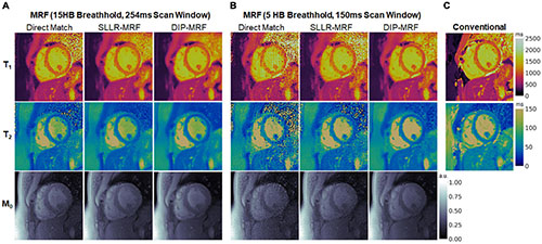
Figure 7. Cardiac MRF T1, T2, and M0 maps from a healthy subject. Maps reconstructed using direct matching, SLLR-MRF, and DIP-MRF are shown for (A) the 15HB/254 ms MRF sequence and (B) the 5HB/150 ms MRF sequence. (C) Conventional MOLLI and T2-prepared bSSFP maps are shown for comparison. All maps were cropped to a 100 × 100 region centered over the heart.
Figure 8 shows examples of spatial basis images from DIP-MRF compared to those from conventional NUFFT gridding and SLLR-MRF. Noise enhancement was observed with NUFFT gridding, especially for the 4th and 5th basis images, which was partially reduced using SLLR-MRF, with DIP-MR yielding the best image quality.
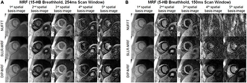
Figure 8. Cardiac MRF spatial basis images from a healthy subject. Spatial basis images from (A) the 15HB/254 ms MRF scan and (B) the 5HB/150 ms MRF scan are shown, reconstructed using (top row) NUFFT gridding, (middle row) SLLR-MRF, and (bottom row) DIP-MRF. Noise enhancement was observed with NUFFT gridding and to a lesser extent SLLR-MRF, while DIP-MRF yielded the best image quality. Although they tend to look similar, the contrasts of the spatial basis images in panels (A,B) are not expected to be identical, as a different subspace (derived from the SVD of a dictionary of signal evolutions) is calculated separately for each scan. All images were cropped to a 100 × 100 region centered over the heart.
Figure 9 demonstrates the effect of training DIP-MRF with different levels of dropout, akin to the simulation results in Supplementary Figure 4. From a visual inspection of the maps, the dropout level that yielded the best noise suppression while preserving high resolution details was 10% for the 15HB/254 ms sequence and 20% for the 5HB/150 ms sequence, when the number of training iterations was fixed at 30,000. Noise enhancement and residual aliasing artifacts were observed at lower dropout levels, whereas overly smoothed maps with loss of fine resolution details were seen at higher dropout levels. Results in two additional subjects are shown in Supplementary Figures 11, 12.
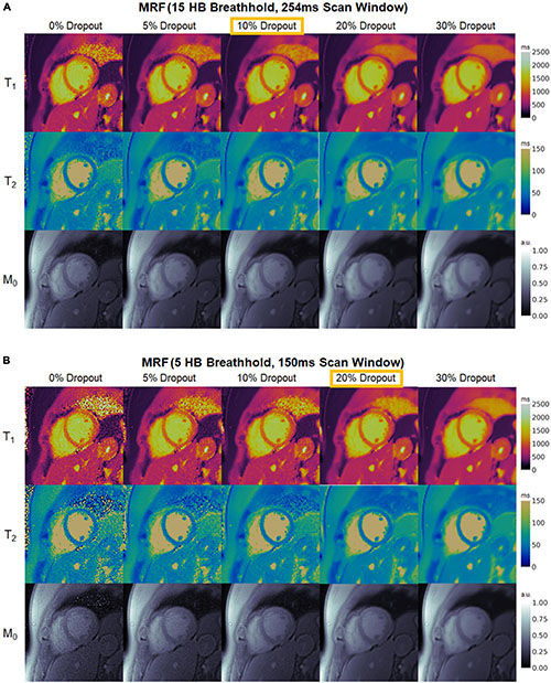
Figure 9. Maps from a healthy subject using DIP-MRF with different levels of dropout during training. The best dropout percentage was determined empirically to be (A) 10% for the 15HB/254 ms MRF sequence and (B) 20% for the 5HB/150 ms MRF sequence. In all cases, the number of training iterations was fixed at 30,000. Using lower dropout led to increased noise and undersampling artifacts, while higher dropout led to overly smoothed maps with a loss of high-resolution details. All maps were cropped to a 100 × 100 region centered over the heart.
Boxplots summarizing the average relaxation times over all subjects in the myocardial septum are shown in Figure 10. T1 values reported as mean ± standard deviation were: MOLLI (1,006 ± 28 ms); 15HB/254 ms MRF with direct matching (1,043 ± 36 ms), SLLR-MRF (1,064 ± 42 ms), and DIP-MRF (1,044 ± 33 ms); and 5HB/254 ms MRF with direct matching (1,065 ± 53 ms), SLLR-MRF (1,072 ± 39 ms), and DIP-MRF (1,035 ± 32 ms). T2 values were: T2-prep bSSFP (47.7 ± 1.6 ms); 15HB/254 ms MRF with direct matching (40.8 ± 3.0 ms), SLLR-MRF (42.3 ± 3.0 ms), and DIP-MRF (41.3 ± 2.9 ms); and 5HB/254 ms MRF with direct matching (46.1 ± 9.0 ms), SLLR-MRF (44.5 ± 3.9 ms), and DIP-MRF (43. ± 3.8 ms). T1 was significantly higher with all MRF techniques compared to MOLLI. T2 was significantly lower with all MRF techniques compared to T2-prep bSSFP, except for the 5HB/150 ms sequence with direct matching. A similar analysis of relaxation times in LV and RV blood is given in Supplementary Figure 14.
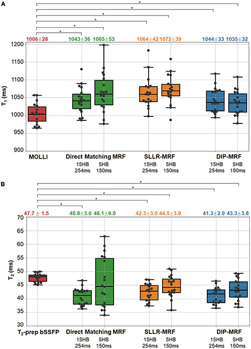
Figure 10. Myocardial T1 and T2 in healthy subject in the left ventricular septum. The boxplots show the distribution of mean (A) T1 and (B) T2 values using MOLLI and T2-prep bSSFP mapping sequences, as well as 15HB/254 ms and 5HB/150 ms MRF sequences with direct matching, SLLR-MRF, and DIP-MRF reconstructions. The top of each box indicates the upper quartile, the bottom indicates the lower quartile, and the horizontal line through the middle shows the median. The numbers above each plot indicate the mean ± standard deviation in milliseconds. Asterisks indicate a significant difference (p < 0.05) using a within-subjects ANOVA test with a Bonferroni post-hoc test for multiple comparisons.
The intersubject variability, quantified as the standard deviation of the mean T1 or T2 over all subjects, was similar among all reconstructions for the 15HB/254 ms MRF scan. For the 5HB/150 ms scan, DIP-MRF yielded a lower intersubject variability (32 ms for T1, 3.8 ms for T2) compared to direct matching (53 ms for T1, 9.0 ms for T2) and SLLR-MRF (39 ms for T1, 3.9 ms for T2), although still higher than conventional mapping sequences (28 ms for T1, 1.5 ms for T2).
Bland-Altman plots comparing relaxation times measured with 15HB/254 ms vs. 5HB/150 ms MRF scans are shown in Figure 11 (note that a positive bias indicates higher measurements using the 5HB/150 ms scan). Both scans yielded good agreement in T1 when using the DIP-MRF reconstruction, with a bias of −9 ms and 95% LoA (−56, 38) ms. Similar results were seen with SLLR-MRF, having a bias of 8 ms and 95% LoA (−41, 58) ms, while a larger bias (22 ms) and wider limits of agreement of (−81, 206) ms were observed with direct matching. DIP-MRF yielded the best agreement between T2 measurements from the 15HB/254 ms and 5HB/150 ms scans, with a bias of 2.0 ms and 95% LoA (−1.9, 6.0) ms. SLLR-MRF had a similar bias (2.1 ms) but wider limits of agreement of (−3.4, 7.7) ms. Direct matching had the largest bias (5.3 ms) and widest limits of agreement (−8.7, 19.4) ms.
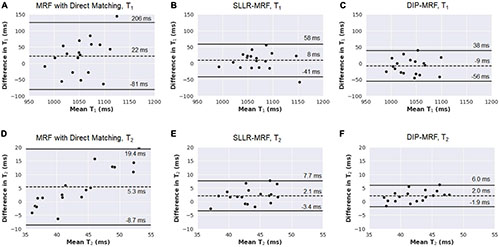
Figure 11. Bland-Altman plots comparing measurements from 15HB/254 ms MRF and 5HB/150 ms MRF scans with different reconstruction methods in healthy subjects. Results are shown for T1 using (A) direct matching, (B) SLLR-MRF, and (C) DIP-MRF. Similar results for T2 are shown in panels (D-F). On each plot, the bias is indicated by a dotted line, and the 95% limits of agreement are indicated by solid lines. Note that a positive bias indicates higher T1 or T2 measurements using 5HB/150 ms MRF compared to 15HB/254 ms MRF.
Figures 12A,B show the spatial distribution of T1 and T2 within individual myocardial segments and over the entire myocardium. Both 15HB/254 ms and 5HB/150 ms MRF scans showed some regional variability in T1 and T2, with higher values in the septum and lower values in the inferolateral segment. A similar but less pronounced trend was seen with MOLLI but not with T2-prepared bSSFP. Greater regional variability was seen with direct matching compared to SLLR-MRF and DIP-MRF.
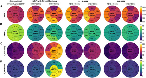
Figure 12. Bullseye plots showing the spatial distribution of T1 and T2 in different myocardial segments of a mid-ventricular slice in healthy subjects. (A) Mean T1 and (B) mean T2 values are shown for mid-ventricular AHA segments, with the value in the center of the bullseye indicating the average over the entire myocardium. The spatial variability (standard deviations) for T1 and T2 within each segment and over the entire myocardium are shown in panels (C,D), respectively.
Figures 12C,D summarize the intrasubject variability for T1 and T2, quantified as the mean of the standard deviations over all subjects, shown within each myocardial segment and over the entire myocardium. Compared to MOLLI (57 ms), the intrasubject variability in T1 over the entire myocardium was significantly higher using the 15HB/254 ms MRF sequence with direct matching (94 ms); this variability was reduced with SLLR-MRF (66 ms) and DIP-MRF (57 ms) and was not significantly different from MOLLI. For the 5HB/150 ms MRF sequence, the intrasubject variability was significantly higher than MOLLI when using direct matching (160 ms) and SLLR-MRF (86 ms); DIP-MRF yielded the lowest variability (61 ms) with no significant difference relative to MOLLI. Compared to T2-prep bSSFP (4.2 ms), the intrasubject variability in T2 over the entire myocardium using the 15HB/254 ms MRF sequence was significantly higher using direct matching (5.6 ms), non-significantly lower using SLLR-MRF (3.9 ms), and significantly lower using DIP-MRF (3.3 ms). For the 5HB/150 ms MRF sequence, the intrasubject variability was significantly higher than T2-prep using direct matching (19.1 ms) and SLLR-MRF (7.1 ms); DIP-MRF yielded the lowest variability (4.1 ms) with no significant difference relative to T2-prep bSSFP.
Patient Scans
Representative maps from a cardiomyopathy patient are shown in Figure 13, with additional patient examples provided in Supplementary Figures 15, 16. In both native and post-contrast maps in patients, DIP-MRF yielded the best suppression of noise and aliasing artifacts, especially for the shortened 5HB/150 ms acquisition, where direct matching led to severe noise and artifacts that were only moderately improved with the SLLR-MRF reconstruction.
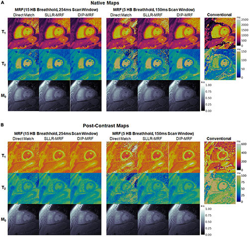
Figure 13. (A) Native and (B) post-contrast T1, T2, and M0 maps from a cardiomyopathy patient. Results are shown for conventional MOLLI and T2-prepared bSSFP sequences, as well as 15HB/254 ms and 5HB/150 ms MRF sequences using direct matching, SLLR-MRF, and DIP-MRF reconstructions. All maps were cropped to a 100 × 100 region centered over the heart.
Figure 14 shows one example of a patient scan where the 15HB breathhold and 254 ms acquisition window resulted in motion artifacts. In this case, motion caused blurring of the myocardial wall and an artifactual increase in septal relaxation times due to partial volume effects between myocardium and blood, with DIP-MRF yielding T1 1263 ± 48 ms and T2 55.8 ± 6.5 ms. To confirm the presence of motion, a sliding window reconstruction was performed (window size = 48 TRs) to visualize one image per heartbeat, shown in Supplementary Figure 17. This analysis confirmed that the patient breathed halfway during the scan, and residual cardiac motion was apparent in the later heartbeats. Motion and partial volume effects were reduced using the shorter 5HB breathhold and 150 ms acquisition window, leading to a sharper depiction of the myocardial wall and lower septal relaxation times of T1 1130 ± 27 ms and T2 48.8 ± 4.1 ms (although T1 and T2 were still elevated compared to healthy subjects). Conventional MOLLI and T2-prep bSSFP mapping values in this patient were T1 = 1,122 ± 47 ms and T2 = 50.1 ± 4.1 ms.
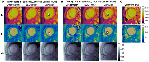
Figure 14. Example of reduced motion artifacts using the shortened 5HB/150 ms MRF acquisition in a cardiomyopathy patient. (A) The myocardial septum (white arrow) appeared blurred using the 15HB/254 ms MRF sequence due to failed breathholding and residual cardiac motion during the acquisition window. (B) Motion artifacts were reduced with the shortened 5HB/150 ms MRF sequence. DIP-MRF yielded improved map quality with less noise compared to the direct matching and SLLR-MRF. (C) MOLLI and T2-prepared bSSFP maps are shown for reference. All maps were cropped to a 100 × 100 region centered over the heart.
Boxplots summarizing the distribution of native and post-contrast relaxation times in the myocardial septum in patients are shown in Figure 15. Using the DIP-MRF reconstruction, both 15HB/254 ms MRF (1,079 ± 72 ms) and 5HB/150 ms MRF (1,047 ± 46 ms) acquisitions yielded higher native T1 than MOLLI (1,033 ± 34 ms); this difference was statistically significant for 5HB/150 ms DIP-MRF. Native T2 was non-significantly lower with both 15HB/254 ms MRF (45.2 ± 5.8 ms) and 5HB/150 ms MRF (45.7 ± 4.0 ms) compared to T2-prep bSSFP (47.6 ± 3.9 ms). Patients had higher native T1 than healthy subjects, but this trend was not significant for MOLLI, 15HB/254 ms MRF, or 5HB/150 ms MRF. Compared to healthy subjects (45.2 ms), native T2 in patients was significantly lower with 15HB/254 ms MRF (41.3 ms) and non-significantly lower with 5HB/150 ms MRF (43.3 ms). No difference between patients and healthy subjects was seen with T2-prep bSSFP (47.6 vs. 47.7 ms). There were no significant differences in post-contrast T1 among MOLLI (417 ± 38), 15HB/254 ms MRF (409 ± 62 ms), or 5HB/150 ms MRF (397 ± 51 ms). Post-contrast myocardial T2 was 37.9 ± 3.0 ms using 15HB/254 ms MRF and 38.7 ± 3.5 ms using 5HB/150 ms MRF (Supplementary Figure 18). Post-contrast T2 bSSFP data were only acquired in a subset of three patients; a comparison of post-contrast T2 bSSFP and MRF in these patients is provided in Supplementary Table 1. An analysis of native and post-contrast relaxation times in LV and RV blood in patients is given in Supplementary Figure 19.
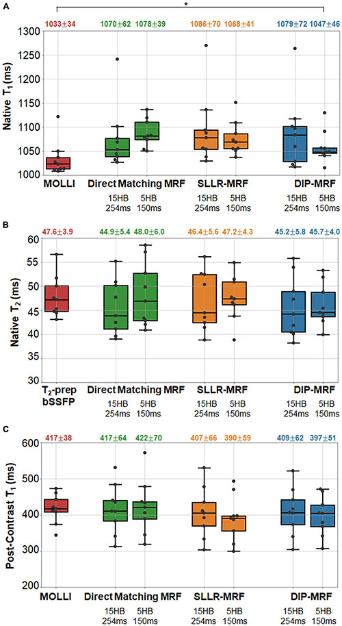
Figure 15. Relaxation times in the myocardial septum in cardiomyopathy patients. The boxplots summarize the (A) native T1, (B) native T2, and (C) post-contrast T1 using conventional mapping sequences, as well as 15HB/254 ms MRF and 5HB/150 ms MRF with direct matching, SLLR-MRF, and DIP-MRF reconstructions. The top of each box indicates the upper quartile, the bottom indicates the lower quartile, and the horizontal line through the middle shows the median. The numbers above each plot indicate the mean ± standard deviation over all patients. Asterisks indicate a significant difference (p < 0.05) using a within-subjects ANOVA test with a Bonferroni post-hoc test for multiple comparisons. Native mapping was performed in all ten patients. Post-contrast MRF was acquired in all ten patients, while post-contrast MOLLI was only collected in nine patients.
Discussion
This study introduced a self-supervised deep learning reconstruction for cardiac MRF, called DIP-MRF, that combines low-rank subspace modeling with the denoising capabilities of a deep image prior. DIP-MRF was shown to reduce noise and aliasing artifacts in tissue property maps compared to conventional dictionary matching and a low-rank subspace reconstruction with spatial and locally low rank constraints (SLLR-MRF). DIP-MRF was leveraged to shorten the breathhold duration of cardiac MRF from 15 to 5 heartbeats and the diastolic acquisition from 250 to 150 ms in vivo, which can potentially reduce motion artifacts, especially for patients who have difficulty performing long breathholds or who have elevated heart rates. By minimizing motion, the shortened acquisition may also decrease partial volume artifacts between myocardium and blood, leading to more accurate and reproducible myocardial T1 and T2 measurements. This effect was demonstrated in Figure 14, where motion resulted in an artifactual increase in myocardial T1 and T2 with the longer MRF scan that was mitigated by shortening the breathhold and scan window.
In most deep learning reconstructions, a neural network is pre-trained using a large number of reference images. For MRF, such training data would consist of “ground truth” tissue property maps (the network output) paired with a time series of undersampled images or k-space measurements (the network input). While it is possible to collect such training data in stationary organs, like the brain, it is more challenging in the heart due to physiological motion and the long scan times that would be required to collect fully-sampled MRF data (on the order of several minutes). Additionally, the fingerprints in cardiac MRF are dependent on the subject’s cardiac rhythm because the scan uses prospective ECG triggering, so many datasets would potentially be needed to ensure the network provides accurate tissue property estimates independent of a patient’s cardiac rhythm. DIP-MRF addresses these challenges by eliminating the need for prior training. Instead, training is performed de novo after each MRF acquisition, and the only requirements for training data are the undersampled k-space measurements from the current scan and the patient’s cardiac rhythm timings from the ECG. The self-supervised training used in DIP-MRF ensures that the reconstructed T1, T2, and M0 maps and spatial basis images are consistent with the acquired k-space data and with a mathematical model of the MRF signal generation and data sampling process.
One limitation of this work is the long computation time of approximately 1.1 h, since training is performed de novo for each scan. Nevertheless, this work used strategies to accelerate the calculation of forward model during training. The spiral k-space data were shifted onto a Cartesian grid using GROG, which allowed use FFT rather than more time-consuming NUFFT operations during training. Without GROG pre-interpolation, the DIP-MRF reconstruction took 5.3 h. A pre-trained Fingerprint Generator Network was also used in place of a Bloch equation simulation to rapidly generate fingerprints for arbitrary T1, T2, and cardiac rhythm timings. The time needed to simulate fingerprints at 1922 voxel locations (the matrix size used for all datasets in this work) was over 8 min using a Bloch simulation (compiled MATLAB Mex code running on 12 parallel CPUs) compared to 30 ms using the Fingerprint Generator Network on a GPU. Future work will explore ways to shorten the computation time of DIP-MRF, possibly to several minutes or less. Transfer learning may be one solution (49), where DIP-MRF is pre-trained using some in vivo scans, and the reconstructed maps are fine-tuned based on the acquired k-space data from the current scan.
In the original DIP publication, early stopping was used to avoid overfitting to noise, and the number of training iterations was manually tuned for each application (27). This study uses dropout to reduce overfitting (43), which allowed the network to be trained for longer and placed less dependence on manually tuning the number of iterations for early stopping. Simulation results showed that dropout improved the reconstruction accuracy and slowed the rate at which overfitting occurred (Supplementary Figure 4). An in vivo dataset was also reconstructed with different dropout levels, while keeping the number of training iterations fixed at 30,000 for simplicity, to empirically determine which settings yielded the best map quality. It was found that the shortened 5HB/150 ms MRF scan benefitted from higher dropout compared to the 15HB/254 ms scan (20 vs. 10% dropout).
In the absence of motion, the 15HB/254 ms and 5HB/150 ms MRF sequences were expected to yield equivalent T1 and T2 measurements. However, large differences were observed using the direct matching reconstruction, which was due to the noise enhancement and aliasing artifacts in maps using the 5HB/150 ms sequence, resulting in the wide limits of agreement in the Bland-Altman plots in Figure 11. Similar discrepancies were seen with SLLR-MRF to a lesser extent. Due to the improved quality of the maps, DIP-MRF yielded the closest agreement in T1 and T2 measured by the 15HB/254 ms and 5HB/150 ms sequences. DIP-MRF also yielded better precision in vivo compared to direct matching and SLLR-MRF. For T1, the intrasubject variability in healthy subjects was similar among MOLLI, 15HB/254 ms DIP-MRF, and 5HB/150 ms DIP-MRF. For T2, the intrasubject variability was lowest for 15HB/254 ms DIP-MRF, and similar between T2-prep bSSFP and 5HB/150 ms DIP-MRF. DIP-MRF also resulted in a lower intersubject variability for T1 and T2 compared to direct matching and SLLR-MRF.
Higher native T1 and lower native T2 were observed using MRF compared to conventional mapping sequences, which has been reported previously (50). MOLLI is known to underestimate T1 (51), and T2-prep bSSFP has been reported to overestimate T2 (52), which was observed in this study in the phantom experiment (Figure 6 and Supplementary Figures 5–7). The signal model in cardiac MRF accounts for slice profile imperfections and inversion pulse efficiency, which was shown to improve accuracy and lead to higher T1 measurements (50). Lower T2 values have been reported with FISP-based MRF sequences compared to standard techniques in other applications, which may be related to magnetization transfer (53), intravoxel dephasing (54), and motion sensitivity along the direction of the unbalanced gradient moment (i.e., slice direction).
Increased regional variability for T1 and to a lesser degree T2 was observed with MRF, with higher relaxation times in the septum and lower values in the inferolateral segment. Possible explanations may include susceptibility effects (especially in the inferolateral segment); partial volume artifacts between myocardium and epicardial fat, which could be improved with water-fat separation techniques like Dixon cardiac MRF (55) or MRF with rosette k-space sampling (56); and B1+ inhomogeneities, which could be addressed using B1+ correction (57, 58). Blood relaxation times were reported for completeness; however, blood flow into and out of the 2D imaging plane is not accounted for in the MRF signal simulation and likely affects the blood T1 and T2 estimates. Interestingly, higher T1 was measured in the LV compared to the RV with both MOLLI and cardiac MRF. Higher T2 was measured in the LV with T2-prep bSSFP, which has been reported previously (59), but slightly lower T2 was measured in the LV with cardiac MRF.
In summary, a DIP-MRF reconstruction that combines low-rank subspace modeling with a deep image prior was shown to reduce noise and aliasing artifacts in cardiac MRF T1, T2, and M0 mapping, which does not require pre-training with in vivo data. This method enables a shortened breathhold duration and cardiac acquisition window in cardiac MRF, which has the potential to improve scan efficiency and reduce motion artifacts. Future work will explore extensions of DIP-MRF to motion-resolved (cine) MRF (60, 61) and 3D cardiac MRF (62).
Data Availability Statement
The raw data supporting the conclusions of this article will be made available by the authors, without undue reservation.
Ethics Statement
The studies involving human participants were reviewed and approved by Institutional Review Boards of the University of Michigan Medical School (IRBMED). The patients/participants provided their written informed consent to participate in this study.
Author Contributions
JH: study conception and design, deep learning reconstruction implementation, data collection and analysis, manuscript preparation, and approved the submitted version.
Funding
This work was supported by the Michigan Institute for Clinical & Health Research (MICHR) Grant UL1TR002240, Siemens Healthineers, and NIH/NHLBI R01HL163030.
Conflict of Interest
This study received funding from Siemens Healthineers (Erlangen, Germany). The funder had no involvement with any aspect of the study design, data collection, interpretation of results, or manuscript preparation.
The author declares that the research was conducted in the absence of any commercial or financial relationships that could be construed as a potential conflict of interest.
Publisher’s Note
All claims expressed in this article are solely those of the authors and do not necessarily represent those of their affiliated organizations, or those of the publisher, the editors and the reviewers. Any product that may be evaluated in this article, or claim that may be made by its manufacturer, is not guaranteed or endorsed by the publisher.
Supplementary Material
The Supplementary Material for this article can be found online at: https://www.frontiersin.org/articles/10.3389/fcvm.2022.928546/full#supplementary-material
References
1. Goldfarb JW, Arnold S, Han J. Recent myocardial infarction: assessment with unenhanced T1-weighted MR imaging. Radiology. (2007) 245:245–50. doi: 10.1148/radiol.2451061590
2. Okur A, Kantarcı M, Kızrak Y, Yıdız S, Pirimoğlu B, Karaca L, et al. Quantitative evaluation of ischemic myocardial scar tissue by unenhanced T1 mapping using 3.0 Tesla MR scanner. Diagn Interv Radiol. (2014) 20:407–13. doi: 10.5152/dir.2014.13520
3. Dall’Armellina E, Piechnik SK, Ferreira VM, Si QL, Robson MD, Francis JM, et al. Cardiovascular magnetic resonance by non contrast T1-mapping allows assessment of severity of injury in acute myocardial infarction. J Cardiovasc Magn Reson. (2012) 14:15. doi: 10.1186/1532-429X-14-15
4. Park CH, Choi E-Y, Kwon HM, Hong BK, Lee BK, Yoon YW, et al. Quantitative T2 mapping for detecting myocardial edema after reperfusion of myocardial infarction: validation and comparison with T2-weighted images. Int J Cardiovasc Imaging. (2013) 29:65–72. doi: 10.1007/s10554-013-0256-0
5. Giri S, Chung YC, Merchant A, Mihai G, Rajagopalan S, Raman SV, et al. T2 quantification for improved detection of myocardial edema. J Cardiovasc Magn Reson. (2009) 11:56. doi: 10.1186/1532-429X-11-56
6. Baggiano A, Boldrini M, Martinez-Naharro A, Kotecha T, Petrie A, Rezk T, et al. Noncontrast magnetic resonance for the diagnosis of cardiac amyloidosis. JACC Cardiovasc Imaging. (2020) 13:69–80. doi: 10.1016/j.jcmg.2019.03.026
7. Sado DM, White SK, Piechnik SK, Banypersad SM, Treibel T, Captur G, et al. Identification and assessment of anderson-fabry disease by cardiovascular magnetic resonance noncontrast myocardial T1 mapping. Circ Cardiovasc Imaging. (2013) 6:392–8. doi: 10.1161/CIRCIMAGING.112.000070
8. Messroghli DR, Walters K, Plein S, Sparrow P, Friedrich MG, Ridgway JP, et al. Myocardial T1 mapping: application to patients with acute and chronic myocardial infarction. Magn Reson Med. (2007) 58:34–40. doi: 10.1002/mrm.21272
9. Weingärtner S, Akçakaya M, Basha T, Kissinger KV, Goddu B, Berg S, et al. Combined saturation/inversion recovery sequences for improved evaluation of scar and diffuse fibrosis in patients with arrhythmia or heart rate variability. Magn Reson Med. (2014) 71:1024–34. doi: 10.1002/mrm.24761
10. Kvernby S, Warntjes MJ, Haraldsson H, Carlhall CJ, Engvall J, Ebbers T. Simultaneous three-dimensional myocardial T1 and T2 mapping in one breath hold with 3D-QALAS. J Cardiovasc Magn Reson. (2014) 16:102. doi: 10.1186/s12968-014-0102-0
11. Akçakaya M, Weingärtner S, Basha TA, Roujol S, Bellm S, Nezafat R. Joint myocardial T1 and T2 mapping using a combination of saturation recovery and T2-preparation. Magn Reson Med. (2016) 76:888–96. doi: 10.1002/mrm.25975
12. Christodoulou AG, Shaw JL, Nguyen C, Yang Q, Xie Y, Wang N, et al. Magnetic resonance multitasking for motion-resolved quantitative cardiovascular imaging. Nat Biomed Eng. (2018) 2:215–26. doi: 10.1038/s41551-018-0217-y
13. Ma D, Gulani V, Seiberlich N, Liu K, Sunshine JL, Duerk JL, et al. Magnetic resonance fingerprinting. Nature. (2013) 495:187–92. doi: 10.1038/nature11971
14. Hamilton JI, Jiang Y, Chen Y, Ma D, Lo WC, Griswold M, et al. MR fingerprinting for rapid quantification of myocardial T1, T2, and proton spin density. Magn Reson Med. (2017) 77:1446–58. doi: 10.1002/mrm.26216
15. Hamilton JI, Pahwa S, Adedigba J, Frankel S, O’Connor G, Thomas R, et al. Simultaneous mapping of T1 and T2 using cardiac magnetic resonance fingerprinting in a cohort of healthy subjects at 1.5T. J Magn Reson Imaging. (2020) 52:1044–52. doi: 10.1002/jmri.27155
16. Cavallo AU, Liu Y, Patterson A, Al-Kindi S, Hamilton J, Gilkeson R, et al. CMR fingerprinting for myocardial T1, T2, and ECV quantification in patients with nonischemic cardiomyopathy. JACC Cardiovasc Imaging. (2019) 12:1584–5. doi: 10.1016/j.jcmg.2019.01.034
17. Cruz G, Qi H, Jaubert O, Kuestner T, Schneider T, Botnar RM, et al. Generalized low-rank nonrigid motion-corrected reconstruction for MR fingerprinting. Magn Reson Med. (2022) 87:746–63. doi: 10.1002/mrm.29027
18. Pierre EY, Ma D, Chen Y, Badve C, Griswold MA. Multiscale reconstruction for MR fingerprinting. Magn Reson Med. (2016) 75:2481–92. doi: 10.1002/mrm.25776
19. Cline CC, Chen X, Mailhe B, Wang Q, Pfeuffer J, Nittka M, et al. AIR-MRF: accelerated iterative reconstruction for magnetic resonance fingerprinting. Magn Reson Imaging. (2017) 41:29–40. doi: 10.1016/j.mri.2017.07.007
20. Doneva M, Amthor T, Koken P, Sommer K, Börnert P. Matrix completion-based reconstruction for undersampled magnetic resonance fingerprinting data. Magn Reson Imaging. (2017) 41:41–52. doi: 10.1016/j.mri.2017.02.007
21. Zhao B, Setsompop K, Adalsteinsson E, Gagoski B, Ye H, Ma D, et al. Improved magnetic resonance fingerprinting reconstruction with low-rank and subspace modeling. Magn Reson Med. (2018) 79:933–42. doi: 10.1002/mrm.26701
22. Assländer J, Cloos MA, Knoll F, Sodickson DK, Hennig J, Lattanzi R. Low rank alternating direction method of multipliers reconstruction for MR fingerprinting. Magn Reson Med. (2018) 79:83–96. doi: 10.1002/mrm.26639
23. Cohen O, Zhu B, Rosen MS. MR fingerprinting deep reconstruction network (DRONE). Magn Reson Med. (2018) 80:885–94. doi: 10.1002/mrm.27198
24. Hamilton JI, Currey D, Rajagopalan S, Seiberlich N. Deep learning reconstruction for cardiac magnetic resonance fingerprinting T1 and T2 mapping. Magn Reson Med. (2021) 85:2127–35. doi: 10.1002/mrm.28568
25. Fang Z, Chen Y, Liu M, Lei X, Zhang Q, Wang Q, et al. Deep learning for fast and spatially-constrained tissue quantification from highly-accelerated data in magnetic resonance fingerprinting. IEEE Trans Med Imaging. (2019) 38:2364–74. doi: 10.1109/TMI.2019.2899328
26. Fang Z, Chen Y, Hung S, Zhang X, Lin W, Shen D. Submillimeter MR fingerprinting using deep learning–based tissue quantification. Magn Reson Med. (2020) 84:579–91. doi: 10.1002/mrm.28136
27. Ulyanov D, Vedaldi A, Lempitsky V. Deep image prior. Proceedings of the IEEE Computer Society Conference on Computer Vision and Pattern Recognition. Washington, DC: IEEE Computer Society (2018). p. 9446–54.
28. Ronneberger O, Fischer P, Brox T. U-Net: convolutional networks for biomedical image segmentation. In: Navab N, Hornegger J, Wells WM, Frangi AF editors. Medical Image Computing and Computer-Assisted Intervention. Berlin: Springer International Publishing (2015). p. 234–41.
29. Chakrabarty P, Maji S. The spectral bias of the deep image prior. arXiv. [Preprint]. (2019). Available online at: https://doi.org/10.48550/arXiv.1912.08905 (accessed March 1, 2022).
30. Baguer DO, Leuschner J, Schmidt M. Computed tomography reconstruction using deep image prior and learned reconstruction methods. Inverse Probl. (2020) 36:094004.
31. Gong K, Catana C, Qi J, Li Q. PET image reconstruction using deep image prior. IEEE Trans Med Imaging. (2019) 38:1655–65. doi: 10.1109/TMI.2018.2888491
32. Lin YC, Huang HM. Denoising of multi b-value diffusion-weighted MR images using deep image prior. Phys Med Biol. (2020) 65:105003. doi: 10.1088/1361-6560/ab8105
33. McGivney DF, Pierre E, Ma D, Jiang Y, Saybasili H, Gulani V, et al. SVD compression for magnetic resonance fingerprinting in the time domain. IEEE Trans Med Imaging. (2014) 33:2311–22. doi: 10.1109/TMI.2014.2337321
34. Lima da Cruz G, Bustin A, Jaubert O, Schneider T, Botnar RM, Prieto C. Sparsity and locally low rank regularization for MR fingerprinting. Magn Reson Med. (2019) 81:3530–43. doi: 10.1002/mrm.27665
35. Hamilton JI, Jiang Y, Ma D, Chen Y, Lo WC, Griswold M, et al. Simultaneous multislice cardiac magnetic resonance fingerprinting using low rank reconstruction. NMR Biomed. (2019) 32: e4041. doi: 10.1002/nbm.4041
36. Hamilton JI, Seiberlich N. Machine learning for rapid magnetic resonance fingerprinting tissue property quantification. Proc IEEE Inst Electr Electron Eng. (2020) 108:69–85. doi: 10.1109/JPROC.2019.2936998
37. Seiberlich N, Breuer FA, Blaimer M, Barkauskas K, Jakob PM, Griswold MA. Non-Cartesian data reconstruction using GRAPPA operator gridding (GROG). Magn Reson Med. (2007) 58:1257–65. doi: 10.1002/mrm.21435
38. Fessler J, Sutton B. Nonuniform fast fourier transforms using min-max interpolation. IEEE Trans Signal Process. (2003) 51:560–74.
39. Walsh D, Gmitro A, Marcellin M. Adaptive reconstruction of phased array MR imagery. Magn Reson Med. (2000) 43:682–90. doi: 10.1002/(sici)1522-2594(200005)43:5<682::aid-mrm10>3.0.co;2-g
40. Jiang Y, Ma D, Seiberlich N, Gulani V, Griswold MA. MR fingerprinting using fast imaging with steady state precession (FISP) with spiral readout. Magn Reson Med. (2015) 74:1621–31. doi: 10.1002/mrm.25559
41. Hargreaves B. Variable-Density Spiral Design Functions. (2005). Available online at: http://mrsrl.stanford.edu/b̃rian/vdspiral/ (accessed June 1, 2017).
42. Winkelmann S, Schaeffter T, Koehler T, Eggers H, Doessel O. An optimal radial profile order based on the golden ratio for time-resolved MRI. IEEE Trans Med Imaging. (2007) 26:68–76. doi: 10.1109/TMI.2006.885337
43. Srivastava N, Hinton G, Krizhevsky A, Sutskever I, Salakhutdinov R. Dropout: a simple way to prevent neural networks from overfitting. J Mach Learn Res. (2014) 15:1929–58.
44. Keenan KE, Stupic KF, Boss M, Russek SE, Chenevert TL, Prasad PV, et al. Comparison of T1 measurement using ISMRM/NIST system phantom. Proceedings of the 24th Annual Meeting of ISMRM. Concord, CA: International Society for Magnetic Resonance in Medicine (2016). p. 3290.
45. Siemens Medical Solutions [SMS].MyoMaps. (2018). Available online at: https://usa.healthcare.siemens.com/magnetic-resonance-imaging/options-and-upgrades/clinical-applications/myomaps (accessed February 27, 2018).
46. Messroghli DR, Radjenovic A, Kozerke S, Higgins DM, Sivananthan MU, Ridgway JP. Modified Look-Locker inversion recovery (MOLLI) for high-resolution T1 mapping of the heart. Magn Reson Med. (2004) 52:141–6. doi: 10.1002/mrm.20110
47. Bland JM, Altman DG. Statistical methods for assessing agreement between two methods of clinical measurement. Lancet. (1986) 1:307–10.
48. Cerqueira MD. Standardized myocardial segmentation and nomenclature for tomographic imaging of the heart: a statement for healthcare professionals from the cardiac imaging committee of the council on clinical cardiology of the American heart association. Circulation. (2002) 105:539–42. doi: 10.1161/hc0402.102975
49. Barbano R, Leuschner J, Schmidt M, Denker A, Hauptmann A, Maaß P, et al. Is deep image prior in need of a good education? arXiv. [Preprint]. (2021). Available online at: https://doi.org/10.48550/arXiv.2111.11926 (accessed March 1, 2022).
50. Hamilton JI, Jiang Y, Ma D, Lo W-C, Gulani V, Griswold M, et al. Investigating and reducing the effects of confounding factors for robust T1 and T2 mapping with cardiac MR fingerprinting. Magn Reson Imaging. (2018) 53:40–51. doi: 10.1016/j.mri.2018.06.018
51. Kellman P, Hansen MS. T1-mapping in the heart: accuracy and precision. J Cardiovasc Magn Reson. (2014) 16:2. doi: 10.1186/1532-429X-16-2
52. Baeßler B, Schaarschmidt F, Stehning C, Schnackenburg B, Maintz D, Bunck AC. Cardiac T2-mapping using a fast gradient echo spin echo sequence - first in vitro and in vivo experience. J Cardiovasc Magn Reson. (2015) 17:67. doi: 10.1186/s12968-015-0177-2
53. Gloor M, Scheffler K, Bieri O. Quantitative magnetization transfer imaging using balanced SSFP. Magn Reson Med. (2008) 60:691–700. doi: 10.1002/mrm.21705
54. Assländer J, Glaser SJ, Hennig J. Pseudo steady-state free precession for MR-fingerprinting. Magn Reson Med. (2017) 77:1151–61. doi: 10.1002/mrm.26202
55. Jaubert O, Cruz G, Bustin A, Schneider T, Lavin B, Koken P, et al. Water–fat Dixon cardiac magnetic resonance fingerprinting. Magn Reson Med. (2019) 83:2107–23. doi: 10.1002/mrm.28070
56. Liu Y, Hamilton J, Eck B, Griswold M, Seiberlich N. Myocardial T1 and T2 quantification and water–fat separation using cardiac MR fingerprinting with rosette trajectories at 3T and 1.5T. Magn Reson Med. (2020) 85:103–19. doi: 10.1002/mrm.28404
57. Ma D, Coppo S, Chen Y, McGivney DF, Jiang Y, Pahwa S, et al. Slice profile and B1 corrections in 2D magnetic resonance fingerprinting. Magn Reson Med. (2017) 78:1781–9. doi: 10.1002/mrm.26580
58. Buonincontri G, Schulte RF, Cosottini M, Tosetti M. Spiral MR fingerprinting at 7T with simultaneous B1 estimation. Magn Reson Imaging. (2017) 41:1–6. doi: 10.1016/j.mri.2017.04.003
59. Emrich T, Bordonaro V, Schoepf UJ, Petrescu A, Young G, Halfmann M, et al. Right/left ventricular blood pool T2 ratio as an innovative cardiac MRI screening tool for the identification of left-to-right shunts in patients with right ventricular disease. J Magn Reson Imaging. (2022) 55:1452–8. doi: 10.1002/jmri.27881
60. Hamilton JI, Jiang Y, Eck B, Griswold M, Seiberlich N. Cardiac cine magnetic resonance fingerprinting for combined ejection fraction, T1 and T2 quantification. NMR Biomed. (2020) 33:e4323. doi: 10.1002/nbm.4323
61. Jaubert O, Cruz G, Bustin A, Schneider T, Koken P, Doneva M, et al. Free-running cardiac magnetic resonance fingerprinting: joint T1/T2 map and cine imaging. Magn Reson Imaging. (2020) 68:173–82. doi: 10.1016/j.mri.2020.02.005
Keywords: deep learning, deep image prior, cardiovascular imaging, low rank, multiparametric magnetic resonance imaging (MRI), magnetic resonance fingerprinting (MRF), T1 mapping, T2 mapping
Citation: Hamilton JI (2022) A Self-Supervised Deep Learning Reconstruction for Shortening the Breathhold and Acquisition Window in Cardiac Magnetic Resonance Fingerprinting. Front. Cardiovasc. Med. 9:928546. doi: 10.3389/fcvm.2022.928546
Received: 25 April 2022; Accepted: 06 June 2022;
Published: 23 June 2022.
Edited by:
Anthony G. Christodoulou, Cedars Sinai Medical Center, United StatesReviewed by:
Ruixi Zhou, Beijing University of Posts and Telecommunications (BUPT), ChinaHaikun Qi, ShanghaiTech University, China
Copyright © 2022 Hamilton. This is an open-access article distributed under the terms of the Creative Commons Attribution License (CC BY). The use, distribution or reproduction in other forums is permitted, provided the original author(s) and the copyright owner(s) are credited and that the original publication in this journal is cited, in accordance with accepted academic practice. No use, distribution or reproduction is permitted which does not comply with these terms.
*Correspondence: Jesse I. Hamilton, hamiljes@med.umich.edu