Local Drivers of Marine Heatwaves: A Global Analysis With an Earth System Model

1. Introduction

Marine heatwaves (MHWs) are anomalously warm and sustained sea surface temperature extremes (Hobday et al., 2016; IPCC, 2019) and have been observed in all ocean basins over the last few decades (Frölicher and Laufkötter, 2018; Oliver et al., 2021). Human-caused climate change has led to observed increases in the frequency, intensity and duration of MHWs over recent decades (Frölicher et al., 2018; Oliver et al., 2018; Oliver, 2019; Laufkötter et al., 2020). These changes are associated with widespread impacts on marine species including changes in their distribution and widespread mortality (Wernberg et al., 2011; Bond et al., 2015; Cheung and Frölicher, 2020; Jacox et al., 2020), loss of biodiversity (Smale et al., 2019), collapses of foundation species such as corals (e.g., Hughes et al., 2017), kelp forests (e.g., Filbee-Dexter and Wernberg, 2018) and sea grasses (e.g., Babcock et al., 2019) and the ecosystems they support (Smale et al., 2019), and declines in fisheries revenues and livelihoods (Cheung et al., 2021). Climate models suggest that ongoing global warming will lead to a continued increase in MHW frequency and intensity (Frölicher et al., 2018), further threatening marine life and the ecosystem services they provide to human societies (Collins, 2019). Hence, it is important to understand the mechanisms driving MHWs.

The main driver of the long-term changes in MHW frequency is the gradual increase in mean ocean temperature (Frölicher et al., 2018; Oliver, 2019). However, the drivers of the onset and decline of individual MHW events are diverse and can differ across regions, seasons and may depend on the persistence of the MHW event. These processes can range from anomalous air-sea heat fluxes or ocean heat advection through changes in atmospheric circulation associated with large-scale teleconnections (Holbrook et al., 2019; Sen Gupta et al., 2020; Oliver et al., 2021) to small-scale local mesoscale processes in the ocean. For example, many prominent and impactful MHWs, such as the Mediterranean Sea 2003 (Olita et al., 2007) and 2006 MHWs (Bensoussan et al., 2010), the Northwest Atlantic 2012 MHW (Chen et al., 2014), the 2013–14 southwest Atlantic MHW (Rodrigues et al., 2019), the Coastal Peruvian 2017 MHW (Echevin et al., 2018) and the Tasman Sea 2017–18 MHW (Perkins-Kirkpatrick et al., 2019) were associated with anomalously high heat fluxes from the atmosphere into the ocean. Other MHWs have been caused primarily by oceanic processes including anomalous horizontal advection of warm waters, such as the Western Australia 2011 MHW (Feng et al., 2013; Benthuysen et al., 2014) and the Tasman Sea 2015–2016 MHW (Oliver et al., 2017). In addition, some MHWs have been caused by a combination of atmospheric and oceanic processes through tropical-extratropical teleconnections, such as the Northeast Pacific 2013–2015 MHW (Bond et al., 2015; Di Lorenzo and Mantua, 2016) and the Southwest Atlantic 2017 MHW (Manta et al., 2018). Some MHWs may have also been caused by small-scale processes, such as ocean mesoscale eddies or synoptic atmospheric weather regimes (Schlegel et al., 2017; Holbrook et al., 2019). MHWs can even be driven by different processes during different seasons as well as during their onset and decline phase. For example, Schlegel et al. (2021) found that MHWs in the Northwest Atlantic tend to be primarily driven by anomalous air-sea heat fluxes during the onset phase, but by oceanic processes during the decline phase. In addition, Schlegel et al. (2021) showed that during cold seasons anomalous air-sea heat fluxes are more important than anomalous horizontal advection for MHW onset and decline in the Northwest Atlantic, while this may be reversed during warm seasons.

Most of the available studies on drivers of MHWs focused on specific individual MHW events and predominantly on atmospheric processes, partly due to the greater availability of such data from satellite records and reanalysis data compared to the sparser coverage of oceanic (sub-)surface measurements. In addition, the studies focusing on ocean processes often apply a mixed layer temperature budget (Oliver et al., 2021), which considers processes that are often not directly measured, such as horizontal diffusion or vertical mixing, as residual terms. Therefore a global view of the dominant local atmospheric and oceanic drivers of MHWs during their onset and decline phases and during different seasons is currently missing. A better physical understanding of why MHWs occur is essential for building and improving the tools for MHW prediction and ultimately for adaptation and ecosystem management (Holbrook et al., 2019).

In this study, we use daily-mean output of all tendency terms that change the surface ocean temperature from a comprehensive coarse-resolution Earth system model to identify and quantify the main local physical processes leading to the onset and decline of MHWs at the global scale and in different seasons (Sections 3.1 and 3.2). We focus on physical processes as simulated in a preindustrial control simulation. We assess also the dependency of these processes on the duration of the MHW event (Section 3.3) and identify groups of MHW events that share similar characteristics of driver processes in certain regions through a clustering approach (Section 3.4). Our modeling framework has the advantage of providing a consistent and physically complete set of temperature tendency terms that are generally not available at a sufficient temporal and spatial resolution from observations and models and are not standard CMIP6 output.

2. Methods

2.1. GFDL ESM2M

The Earth system model used in this study is the global coupled carbon-climate model ESM2M developed at the National Oceanic and Atmospheric Administration (NOAA)'s Geophysical Fluid Dynamics Laboratory (GFDL) (Dunne et al., 2012, 2013). The GFDL ESM2M consists of an ocean model (MOM4p1; Griffies, 2009), an atmosphere model (AM2; Anderson et al., 2004), a land model (LM3.0; Milly et al., 2014), a sea ice model (Winton, 2000), and also includes iceberg dynamics (Martin and Adcroft, 2010). The ocean model MOM4p1 uses a tripolar horizontal grid with a nominal resolution of 1° increasing zonally to 1/3° near the equator. Its vertical grid has 50 levels with a time-dependent resolution of about 10m in the upper 230m of the water column. The atmospheric model AM2 has a horizontal grid resolution of 2° × 2.5° with 24 vertical levels.

We analyze daily mean sea surface temperature (SST) data averaged over the top 10 m of the ocean and its drivers from a 500-yr long preindustrial control simulation (Burger et al., 2020). Atmospheric CO₂ and all non-CO₂ radiative forcing agents were kept constant at their preindustrial levels. The model is in quasi-equilibrium with the preindustrial forcing, i.e., there is no long-term drift in global mean SST over the 500-yr simulation (slope of least squares linear regression is 0.006 K/100 y). The preindustrial control simulation was used due to the large available sample size, i.e., 500 years of daily-mean output data. However, the main results were confirmed with an eight-member ensemble simulation of the GFDL ESM2M (Burger et al., 2020) forced by historical and Representative Concentration Pathway 8.5 (RCP8.5) forcings over the period 1982–2021 (Supplementary Figure 1).

2.2. Marine Heatwave Definition

We define an MHW as a period during which the SST at a location is larger than a seasonally varying threshold given by the local 90th percentile of SST anomalies (relative to the mean seasonal cycle) that is calculated for each calendar day individually (Figure 1). Under this definition, MHWs may occur with the same frequency throughout the year and at all locations. We applied this definition to each ocean grid cell individually and do not consider the potential spatial coherence of events. Our definition is similar to the widely-used MHW definition by Hobday et al. (2016), but in contrast to their definition, we do not apply a duration threshold of at least 5 consecutive days and we do not fill in short gaps in SST threshold exceedance. We then calculate the maximal or mean magnitude of an MHW event as the maximal or mean SST anomaly relative to the mean seasonal cycle over the duration of a single event (Figure 1), respectively.

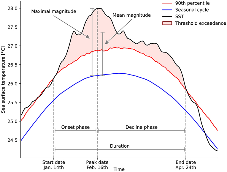
Figure 1. Schematic figure illustrating the definition of a marine heatwave (MHW) and associated characteristics used in this study. The time series of simulated sea surface temperature (SST) averaged over the 55°E–105°E and 15°S–30°S region in the subtropical Indian Ocean for year 175 of the preindustrial control simulation is shown in black. The climatological seasonal cycle is shown in blue and the 90th percentile threshold in red. The red shaded area indicates the occurrence of the MHW. The period between the start (Jan 14th) and the peak (Feb 16th) of the MHW is labeled as the onset phase. The period between the peak and the end (Apr 24th) is labeled as the decline phase. The time span between start and end indicates the duration. Also shown are the maximum magnitude (maximal SST anomaly relative to the seasonal cycle) and the mean magnitude (SST anomaly averaged over the duration of the event).

For each MHW, we identify an onset and decline phase (Figure 1; Hobday et al., 2016; Schlegel et al., 2021). The onset phase is the period between the MHW start date, i.e., the first day when the SST is above the seasonally varying extreme event threshold, and the MHW peak date, i.e., when the MHW magnitude is at its maximum. The decline phase of an MHW is the period between the peak date and the end date, i.e., when the SST falls below the seasonally varying extreme event threshold. This separation of MHWs into two phases allows an analysis of the driving processes of the onset and decline of MHWs individually, as the processes can be different for these two phases (Schlegel et al., 2021). The MHW peak provides a natural midway point. We note that long MHWs can have multiple local maxima with no single clear peak, in which case this method does not clearly separate “onset behavior” from “decline behavior”. However, this potentially distorting effect is averaged out by the large number of MHWs per grid cell over the full 500-yr simulation period. The identification of two phases requires a minimum duration of 2 days, which we therefore apply in all following analyses where a distinction between onset and decline phases is made. The exclusion of 1-day events does not greatly affect the results since they make up only 1.2% of all MHWs on global average.

2.3. Model Evaluation

The GFDL ESM2M model simulates well the observed amplitude and spatial patterns of MHW mean magnitude (Figures 2A–C) as well as the changes in MHW days per year, magnitude and duration over the 1981-2019 satellite period (Frölicher et al., 2018; Gruber et al., 2021). The global mean simulated MHW magnitude of 1.2 K in GFDL ESM2M is very close to the observation-based estimate of 1.3 K in the NOAA OISST v2.1 sea surface temperature dataset (Huang et al., 2020). Regionally, the model reproduces well the relatively small observed MHW mean magnitude in the subtropics and higher magnitudes in the eastern equatorial Pacific and the northern high latitudes. However, there exist biases in simulated magnitude around Antarctica, the tropical Pacific and the western boundary currents of both hemispheres. The biases in the western boundary currents are a common problem across the whole model ensemble that participated in the Coupled Model Intercomparison Project Phase 5 (Frölicher et al., 2018) and Phase 6 (Plecha and Soares, 2020), and can be attributed to the relatively low horizontal and vertical resolution of its atmospheric and in particular oceanic models (Pilo et al., 2019). The western boundary current regions exhibit intense small-scale and coastal interactions, which are more skilfully simulated by higher-resolution models (Hayashida et al., 2020).

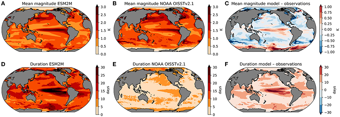
Figure 2. Comparison between simulated and observed marine heatwave mean magnitude (top row) and duration (bottom row). The marine heatwave metrics are calculated from (A,D) the 500-yr preindustrial control simulation and (B,E) the NOAA OISST v2.1 dataset spanning the period from September 1st 1981 to December 24th 2020. The NOAA OISST v2.1 dataset is a blend of satellite and in situ ship, buoy, and Argo float sea surface temperature observations interpolated onto a global 1/4° resolution grid (Huang et al., 2020). (C,F) Differences between simulated and observation-based estimate. The NOAA OISST data was regridded onto the MOM4p1 grid after computing MHW metrics for comparison. Results for the GFDL ESM2M are similar when using a 1981–2021 reference period (not shown).

The duration of MHWs is less well-simulated in GFDL ESM2M than the mean MHW magnitude (Figures 2D–F). The global mean duration of MHWs in GFDL ESM2M is 15.0 days (median: 13.9 days). This is more than three times longer than the observation-based MHW mean duration of 4.6 days (median: 4.5 days). Similar biases toward too long lasting MHW events have been identified across all models analyzed in the CMIP5 and CMIP6 generation (Frölicher et al., 2018; Plecha and Soares, 2020), irrespective of their horizontal and vertical resolution (Pilo et al., 2019). The observation-based estimate may be skewed toward the short side because of missing observations in the SST products that may lead to artificial breaks in MHWs (Schlegel et al., 2019), but this effect is likely secondary to the model's own bias in simulating short-term SST variability. Further possible reasons for this difference are the fact that satellite measurements are snapshots in time while model output consists of daily averages, and that simulated variables here are averages over the top 10 meters, whereas the satellite data represent sea surface skin temperature. If the modeled and observation-based durations are normalized by their respective global mean values, the relative spatial pattern is well-simulated (not shown). The overestimation of MHW duration in the model could generally favor heat budget terms that vary on longer time scales and thereby cause a bias in the identified MHW drivers. However, the relatively weak dependence of the MHW drivers on event duration (see Section 3.3) indicates that the overestimation of MHW duration does not lead to such a bias in MHW drivers.

The simulated biases for both duration and magnitude shown in Figure 2 are similar in spatial pattern but slightly reduced in magnitude when using an eight-member ensemble simulation of the same model for the 1982–2021 period under historical and RCP8.5 forcing (not shown). The relatively good agreement between modeled and observation-based climatological MHW characteristics and trends (Frölicher et al., 2018), apart from the duration, and the model's fidelity in simulating mean state (Bopp et al., 2013) and interannual variability in SST (Suarez-Gutierrez et al., 2021) gives us confidence in using the GFDL ESM2M model for analyzing the drivers of MHWs at the global scale.

2.4. Driver Analysis

To assess the local physical drivers of MHWs, we make use of the temperature tendency terms available in MOM4p1 (Griffies and Greatbatch, 2012; Palter et al., 2014, 2018; Griffies et al., 2015, 2016). In each grid cell, the model decomposes the change in heat (ΔQ_total) between time steps into a number of different heat budget terms, which represent changes in temperature arising from different processes represented in the model. The total heat tendency at the sea surface, in units of W m-2, is given by:

ΔQ_a-s is the air-sea exchange of heat including net shortwave (net incoming surface shortwave radiation minus the shortwave radiation fraction that penetrates beneath the surface layer; Manizza et al., 2005) and net incoming longwave radiation, as well as net latent and sensible heat fluxes. The absorption of shortwave radiation from organic matter within the water column is taken into account based on the chlorophyll concentration that is simulated by the ocean biogeochemistry component TOPAZv2 (Dunne et al., 2013). ΔQ_vmix is the heat flux arising from the non-local part of the K-profile parameterization (KPP; Large et al., 1994), which represents convective vertical mixing in the ocean boundary layer under negative surface buoyancy forcing (herein referred to as convective vertical mixing). ΔQ_vdiff represents heat fluxes due to vertical diffusion and also includes vertical mixing in the ocean boundary layer from the local part of the K-Profile parameterization and tidal mixing (herein referred to as vertical diffusion). ΔQ_adv is the heat change due to horizontal and vertical advection, including both resolved and parameterized subgrid-scale advective heat fluxes (Griffies, 1998; Fox-Kemper et al., 2008). Other smaller terms, such as heat exchange through liquid runoff from rivers, solid runoff from iceberg calving, neutral diffusion, or heat flux resulting from water exchange across the surface due to precipitation minus evaporation are included in the residual heat flux term (ΔQ_res). More details on all 17 heat budget terms included in MOM4p1 can be found in the Supplementary Table 1. As the term ΔQ_res is small and hardly contributes to the temperature changes during MHWs, ΔQ_total can be approximated as

A change in heat content is then converted into a change in potential temperature (Δθ; in units of K s-1) using

where $C_p^0$ is a constant heat capacity of 3992.1 J kg-1 K-1 used in MOM4p1, ρ₀ is the constant Boussinesq density (1.035 kg m-3), and dz is the time-varying vertical grid cell thickness (in units of m) (Griffies, 2015). Here, we assume a constant thickness of dz= 10 m, leading to a conversion factor of 0.002 09 K m2 s-1 W-1. This assumption is valid since actual dynamic variations in grid cell thickness deviate only slightly from this value (maximal variations of order 1 × 10⁻² m in the open ocean) and lead only to small changes in the conversion factor. For a heat flux of 150 W m-2, a grid cell thickness variation of 1 × 10⁻² m translates to an error of only 0.06 K d-1.

Δθ slightly differs from the simulated changes in SST, because the tendencies in the model are only available at daily-mean resolution, whereas the ocean model time-step is 2 h, and these errors can accumulate over time. However, the time mean absolute difference over the full 500 years between the SST simulated by the model and the SST computed from daily-mean temperature tendency terms is less than 0.2 K over 91.7% of the ocean area. Over timescales on the order of MHW durations, this error is even further reduced: the mean error over a 100-day period is smaller than 0.01 K over 99.9% of the ocean area as estimated from n = 1, 000 randomly selected 100-day periods. Therefore, these small differences do not affect the main results of our study.

We computed the anomalies of all temperature tendency terms relative to their seasonal cycles at each grid cell. These anomalies were then separately averaged over all days during the onset phase and over all days during the decline phase, respectively. Terms with positive anomalies during onset phases increase temperature anomalies and thus support MHW formation, while terms with positive anomalies during decline phases counteract MHW decline. In order to detect seasonal differences in driver patterns, the terms were also averaged over MHW days that occur in summer or winter only. Here, the summer season is defined as the months June-July-August (JJA) in the Northern Hemisphere and December-January-February (DJF) in the Southern Hemisphere, and vice versa for the winter season.

We also analyze the individual terms that contribute to ΔQ_a-s, such as net incoming shortwave radiation, net incoming longwave radiation and latent and sensible heat flux, as well as potential drivers of these terms such as total cloud amount (e.g., impacting shortwave and longwave radiation) and wind stress (e.g., impacting latent and sensible heat fluxes). As these terms were not available in the 500-yr preindustrial control simulation, an additional 100-yr preindustrial control simulation was performed with daily-mean output for the individual terms that contribute to ΔQ_a-s. This additional data is only used in Figure 4 and Supplementary Figure 2.

2.5. Regional MHW Classification

MHWs are assigned to different “MHW types” by applying the K-Means clustering algorithm to all MHWs in different ocean regions separately. K-Means clustering is a statistical procedure operating on a set of n data points on p coordinates and identifies a prescribed number K of clusters of data points such that the squared Euclidean distance between members within each cluster is minimized (James et al., 2014). This has the conceptual effect of identifying groups of data points (in this case: MHWs) that are similar to one another based on their coordinate values. The coordinates used to characterize events for clustering were the different drivers of MHWs (see Equation 2), i.e., anomalies of ΔQ_a-s, ΔQ_vmix, ΔQ_vdiff, and ΔQ_adv, each averaged over both the onset and decline phases of each MHW, respectively. Thus, each MHW is characterized by eight numbers and can be quantitatively compared to other MHWs, and the clusters found by the algorithm are interpreted as distinct types or classes of MHWs. Since the clustering algorithm was applied to the set of MHWs in each region separately, the resulting clusters (MHW types) are not necessarily related across regions. The clustering algorithm is not fully deterministic in the sense that repeated clustering of the same input data may result in different clusters being detected, since the algorithm is initialized by choosing random starting cluster centroids (James et al., 2014). However, we found that repeated clustering does not lead to substantially different clusters implying that our method is robust. We chose a value of K = 3 for the number of types identified in order to obtain a set of types that is large enough to allow for a sufficient representation of the driver variability among events while being small enough to be able to be communicated in a comprehensive manner.

3. Results

3.1. MHW Drivers During Onset Phase

We first analyze the annual mean drivers of the onset of MHWs at the global scale. The global annual mean heat flux anomalies in the surface ocean layer are summarized in Table 1. During the MHW onset phase, the global annual mean surface ocean heat gain is 18.1 W m-2. This heat gain is driven by strongly opposing processes. The dominant driving process for the temperature increase is reduced ocean heat loss to the atmosphere, i.e., net ocean heat uptake. In the climatological annual mean state averaged over the 500-yr preindustrial control simulation, the ocean is losing heat to the atmosphere and the layer beneath the surface (Figure 3A). However, during the onset phase, this ocean heat loss is reduced and contributes 29.8 W m-2 (or +165%) to the total heat gain of 18.1 W m-2. A decrease in vertical diffusion and local mixing of heat from the local part of the KPP boundary layer scheme to the subsurface (6.8 W m-2 or +38%) and an increase in advection of warm waters (2.2 W m-2 or +12%) also contribute to the increase in temperature during the onset phase, but their mean contributions are relatively small at global scale and on annual average. The main counteracting process during the onset phase is convective vertical mixing from the non-local part of the KPP boundary layer scheme. In the climatological mean state, convective vertical mixing enhances the surface ocean heat content through mixing of warm subsurface waters to the surface (Figure 3D), but it is reduced during the MHW onset (-20.9 W m-2 or −115%).

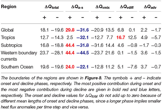
Table 1. Annual mean contributions of the different processes (in W m-2) to the onset and decline of marine heatwaves averaged over the global ocean, tropics, subtropics, western boundary currents, and Southern Ocean.

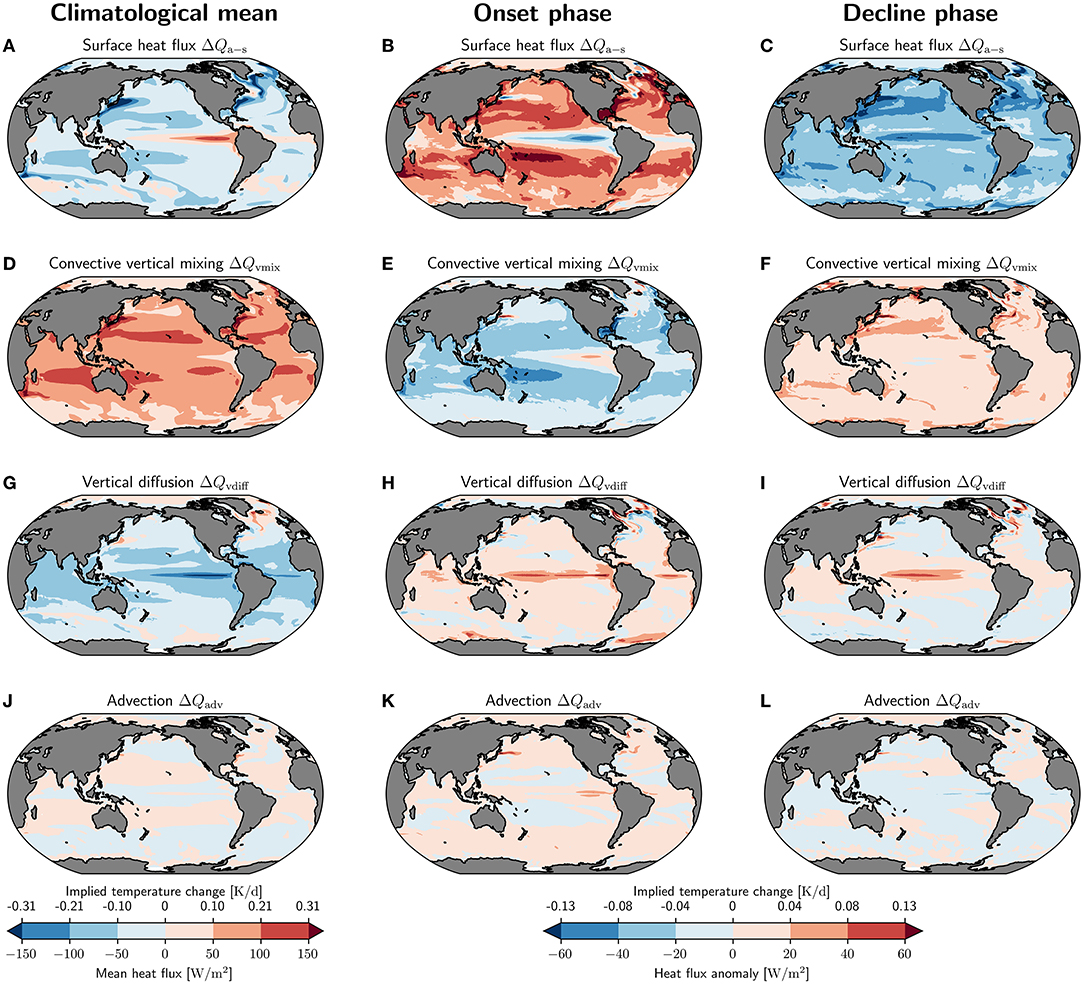
Figure 3. Simulated patterns of the four most important heat and temperature tendency terms averaged over the 500-yr preindustrial control simulation [labeled as climatological mean; (A,D,G,J)], during the onset phase of marine heatwaves (B,E,H,K), and during the decline phase of marine heatwaves (C,F,I,L). The patterns during the onset and decline phase were obtained by averaging daily surface tendency term anomalies of each term over all onset and decline days of marine heatwaves, respectively. Implied temperature changes (units of K d^-1) were computed assuming a constant grid cell thickness, see Section 2.4.

Next, we analyze the regional patterns of the drivers during the onset of MHWs starting with the mid-to-high latitudes.

The anomalous net ocean heat uptake is positive over 92.5% of the ocean surface area during the onset phase with maximum positive anomalies in the mid-latitudes between 15° and 40° in both hemispheres, as well as in the northeastern North Atlantic (Figure 3B). The annual mean net ocean heat uptake during the onset of MHWs in the mid-latitudes is associated with reduced latent heat loss to the atmosphere (green line in Figure 4A) due to decreased wind stress magnitude (dash-dotted gray line in Figure 4A). The direction of the wind stress anomaly during the onset of MHWs is often opposed to the climatological mean wind stress direction in these regions (not shown). In the higher latitudes north of 47°N and south of 57°S, the net ocean heat uptake is mainly associated with increased net shortwave radiation (blue line in Figure 4A) due to less cloud cover (dotted pink line in Figure 4A). The positive anomalies from net ocean heat uptake (Figure 3B) are strongly damped by negative heat flux anomalies arising from a decrease in convective vertical mixing (Figure 3E). These two terms are strongly negatively correlated in time over most of the ocean surface area, with a global mean Pearson correlation coefficient of r = −0.7. This is due to the nature of the convective vertical mixing term implemented in the ocean model MOM4p1, which is given by the non-local KPP parameterization, to counteract air-sea heat fluxes in circumstances of negative buoyancy forcing (Griffies, 2012). Vertical diffusion and advection play a negligible role in the mid-to-high latitudes in the annual mean, except in the western boundary currents of the northern hemisphere, where the advection of heat contributes to the onset of MHWs. The potential of advection-driven MHWs in these regions results from the strong currents and sharp horizontal temperature gradients in the western boundary current regions. However, the GFDL ESM2M model used in this study has a too coarse resolution to resolve mesoscale processes that play a substantial role in the dynamics of the ocean in these regions (Hayashida et al., 2020), and may therefore underestimate the impact of advection.

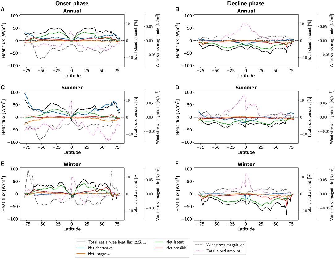
Figure 4. Individual contributions to air-sea heat flux anomalies during marine heatwave onset and decline for the annual mean (A,B), summer (C,D), and winter (E,F) season. Shown are zonal mean air-sea heat flux anomalies ΔQ_a-s, as well as the air-sea heat flux component anomalies (shortwave and longwave radiation, latent and sensible heat fluxes), wind stress magnitude anomalies, and total cloud amount anomalies. The summer and winter panels show the anomalies averaged over the respective season in both hemispheres simultaneously. For summer, the panels use JJA for the Northern Hemisphere and DJF for the Southern Hemisphere. For winter, the panels use DJF for the Northern Hemisphere and JJA for the Southern Hemisphere. The climatological mean state for these terms in the annual mean and during summer and winter is given in Supplementary Figure 2.

In the tropics, the drivers of the onset of MHWs are different from those in the mid-to-high latitudes. In fact, the ocean heat uptake is reduced in the central and eastern equatorial Pacific during the onset of MHWs (Figure 3B). When averaged over the entire equatorial region between 5°S and 5°N, the ocean loses a small amount of heat to the atmosphere (black line in Figure 4A), since the incoming shortwave radiation is slightly reduced (blue line in Figure 4A) due to enhanced total cloud amount (pink dotted line in Figure 4A) and since the anomalies in the latent heat fluxes are small compared to the mid-to-high latitudes (green line in Figure 4A). As opposed to other regions, the onset of MHWs in the equatorial region is driven by positive contributions of enhanced convective vertical mixing (Figure 3A) and in particular of reduced vertical diffusion (Figure 3H). A positive anomaly in the vertical diffusion heat flux indicates that diffusive and local mixing heat loss to the subsurface is less efficient. In the central equatorial Pacific, this is consistent with reduced wind stress during the MHW onset (not shown), which increases stratification and thus reduces the vertical transfer of heat through diffusion and local mixing.

Finally, we analyze the drivers of the onset of MHWs for the summer months and winter months separately (Figures 4C,E, 5). In general, the patterns are qualitatively similar between summer and winter for all terms except vertical diffusion (Figure 5). The net ocean heat uptake dominates the onset of MHWs during both winter and summer season (Figures 5A,B), similarly to the annual mean (Figure 3B). The decrease in convective vertical mixing counteracts the warming (Figures 5C,D), although in some regions such as in the northern North Atlantic, the convective vertical mixing can become a positive driver in winter.

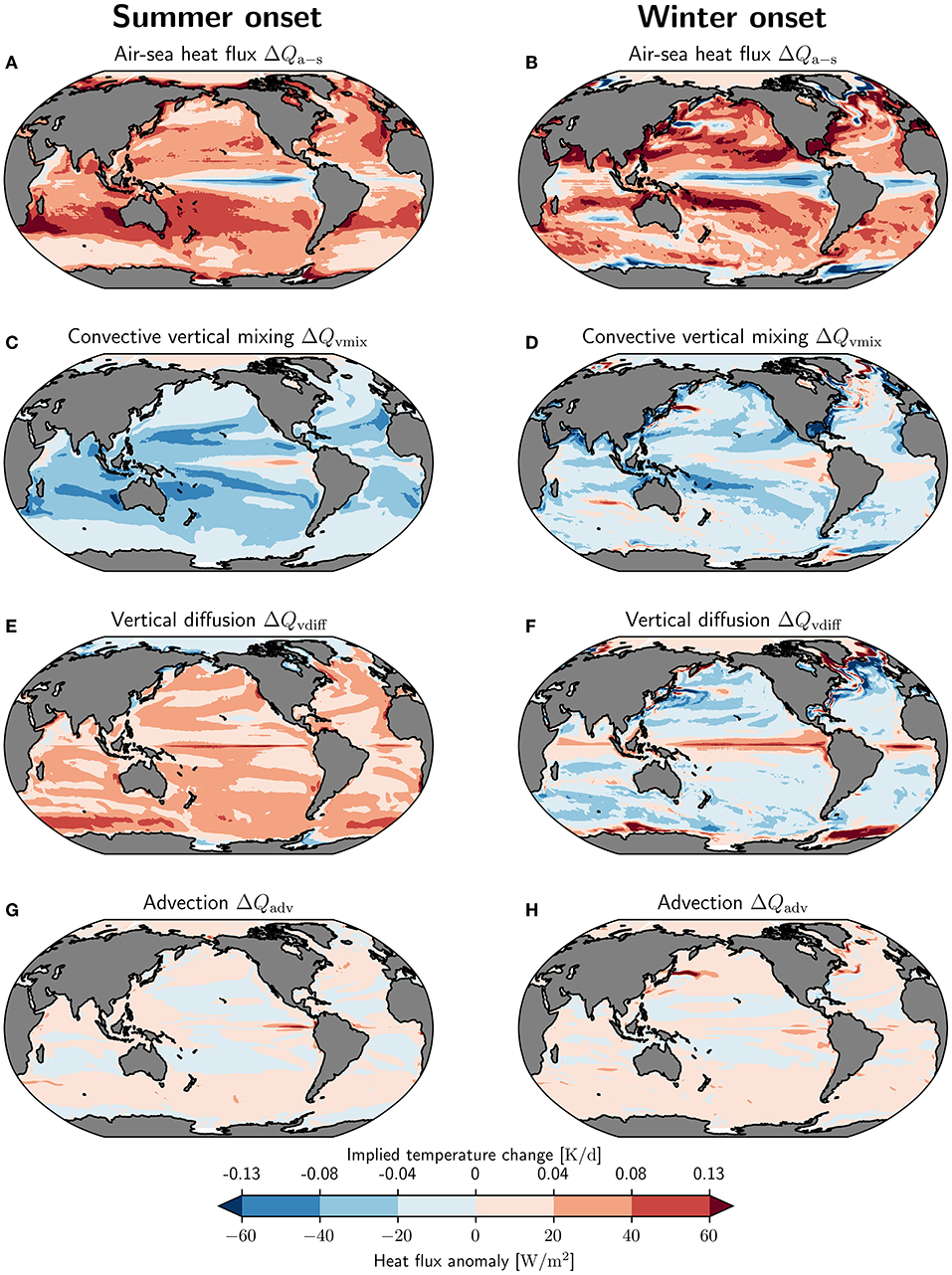
Figure 5. Seasonal decomposition of marine heatwave driver anomaly patterns during the onset phase. Heat flux anomalies for the four most important marine heatwave drivers averaged over marine heatwave onset days during summer (A,C,E,G) and winter (B,D,F,H). The summer and winter maps show the anomalies averaged over the respective season in both hemispheres simultaneously, i.e., for summer (winter), the maps use JJA (DJF) for the Northern Hemisphere and DJF (JJA) for the Southern Hemisphere. The climatological mean state for these terms during summer and winter is given in Supplementary Figure 3.

Despite these general similarities between winter and summer months, there are subtle differences in the local drivers between the seasons. For example, the drivers of the air-sea heat fluxes show pronounced differences between the seasons (Figures 4C,E). During the onset of MHWs in summer, the net ocean heat uptake is mainly driven by reduced latent heat loss (green line in Figure 4C) and increased incoming shortwave radiation, especially in the higher latitudes (blue line in Figure 4C). During the onset of MHWs in winter, however, the reduced latent heat loss (green line in Figure 4E) is reinforced by a reduction in sensible heat loss (red line in Figure 4E). The reduction in sensible heat loss is possibly related to a reduction in surface wind stress (gray dash-dotted line in Figure 4E) and a decrease in the air-sea temperature gradient (e.g., due to anomalous high surface air temperature). In addition, the net ocean heat uptake is almost zero during winter in the very high latitudes (black line in Figure 4E), in contrast to the relatively high net ocean heat uptake during summer months (black line in Figure 4C). Besides the components of the air-sea heat flux, the vertical diffusion also reveals noticeable seasonality (Figures 5E,F), except in the equatorial region. During the onset of MHWs in summer, reduced vertical diffusion acts to warm the surface ocean (Figure 5E), whereas in winter, enhanced vertical diffusion in the mid-to-high latitudes acts to cool the surface ocean (Figure 5F). Advection plays a negligible role in summer, but can contribute to the onset of MHWs in winter in the western boundary currents of the Northern Hemisphere.

3.2. MHW Drivers During Decline Phase

The annual mean decline of MHWs, like the onset, is predominately driven by anomalous atmosphere-ocean heat exchange (Table 1). The global annual mean ocean heat loss anomaly to the atmosphere during the decline phase is -31.6 W m-2 (or 161% of the total heat loss). The main counteracting process is the increase in convective vertical mixing (13.5 W m-2 or −69%). Advection (-1.7 W m-2; or 9%) and vertical diffusion (0.1 W m-2; or 1%) play a secondary role for the decline of MHWs at the global scale in the annual mean.

Anomalous annual mean surface ocean heat loss to the atmosphere occurs everywhere in the global ocean during the decline of MHWs (Figure 3C), mostly due to increased latent heat loss to the atmosphere (green line in Figure 4B). This is different from the onset phase, where the air-sea heat flux anomaly in the equatorial region and especially in the central-to-eastern equatorial Pacific was opposite to that in the rest of the ocean (Figure 3B). In the equatorial region, the negative anomaly in air-sea heat flux during the onset phase also prevails during the decline phase, associated with increased latent heat loss (green line in Figure 4B) and decreased incoming shortwave radiation (blue line in Figure 4B) due increased total cloud cover (pink dotted line in Figure 4B). Particularly strong negative anomalies in air-sea heat fluxes are simulated in the tropics and the mid-latitudes of the Northern Hemisphere (Figure 3C and Table 1).

The increase in convective vertical mixing and associated warming counteracts the cooling induced by surface ocean heat loss to the atmosphere in almost all regions in the annual mean (Figure 3F). This dampening effect of convective mixing is largest in regions where the anomalous surface heat flux is also largest. An exception is the equatorial Pacific, where the large negative surface heat flux anomalies are accompanied by only small positive vertical mixing contributions. This suggests again that the upwards heat transport by convective vertical mixing is inhibited by enhanced stratification in the tropics during MHWs. A decrease in vertical diffusion and local mixing and associated warming in the central equatorial Pacific is not only prevalent in the onset phase, but also in the decline phase (Figure 3I). The persistence of positive heat flux anomalies from vertical diffusion in the central equatorial Pacific also suggests lasting effects from stratification in this region, as vertical diffusion of heat downwards into the water column could be suppressed by stratification over the entire duration of MHW events. However, over most of the extratropics, heat flux from vertical diffusion is now anomalously negative. Advective heat flux anomalies are smaller than the other three terms in all ocean regions (Figure 3L).

The seasonal drivers for the decline of MHWs are broadly similar to the drivers for the annual mean. During winter and summer, the net heat loss to the atmosphere dominates the temperature decline (Figures 6A,B) and the increase in convective vertical mixing counteracts this cooling (Figures 6C,D). Similarly as during the onset of MHWs, the seasonality of the local drivers during the decline is most pronounced for the vertical diffusion (Figures 6E,F) and the components of the net ocean heat loss (Figures 4D,F). In summer, the increased vertical diffusion and local mixing reinforces the cooling of the surface ocean during the decline of MHWs in the mid-to-high latitudes (Figure 6E). In winter, however, reduced vertical diffusion and local mixing in mid-to-high latitudes (Figure 6F) and enhanced convective vertical mixing (Figure 6D) counteracts the cooling during the decline of MHWs. The net ocean heat loss in both seasons is dominated by increased latent heat loss (Figures 4D,F). During winter and in high latitudes, the decline of MHWs may be dominated by the increase in sensible heat loss.

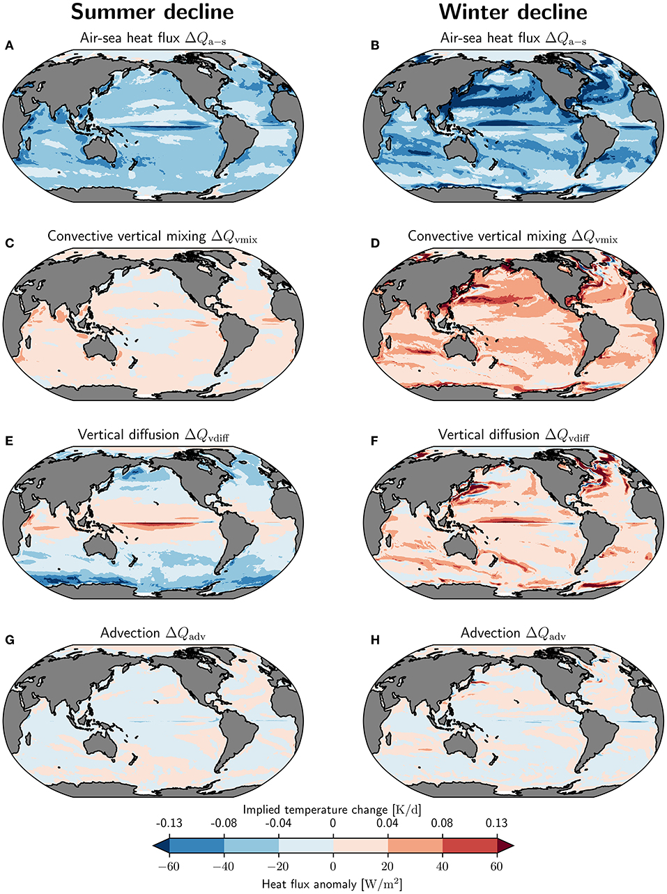
Figure 6. Seasonal decomposition of marine heatwave driver anomaly patterns during the decline phase. Heat flux anomalies for the four most important marine heatwave drivers averaged over marine heatwave decline days during summer (A,C,E,G) and winter (B,D,F,H). The summer and winter maps show the anomalies averaged over the respective season in both hemispheres simultaneously, i.e., for summer (winter), the maps use JJA (DJF) for the Northern Hemisphere and DJF (JJA) for the Southern Hemisphere. The climatological mean state for these terms during summer and winter is given in Supplementary Figure 3.

3.3. Driver Dependence on MHW Duration

The relative importance of each driver's contribution to the total heat flux anomaly during MHW onset and decline does not strongly depend on MHW duration (Figure 7). In other words, the processes leading to the onset and decline of MHWs are similar for short MHWs and for long MHWs. For example, the onset of very short (2–3 day long) MHWs in the global tropics is mainly driven by positive ocean heat uptake anomalies (139%) and vertical diffusion (101%), and damped by convective vertical mixing (−137%) (Figure 7A). This relative contribution of drivers is very similar for long (40–531 days long) MHWs: 115% for ocean heat uptake, 98% for vertical diffusion, and −116% for convective vertical mixing. In some regions, the relative contributions of the drivers increase with increasing duration. For example, the onset of long (28–487 days) MHWs in the subtropics has a stronger relative contribution of positive ocean heat uptake anomalies that is counteracted by a stronger negative contribution of convective vertical mixing than for the onset of short MHWs (Figure 7C). This reinforcing effect of the drivers under longer MHWs is also simulated during the onset in the western boundary currents (Figure 7E) and during decline in tropics, subtropics and western boundary currents (Figures 7B,D,F).

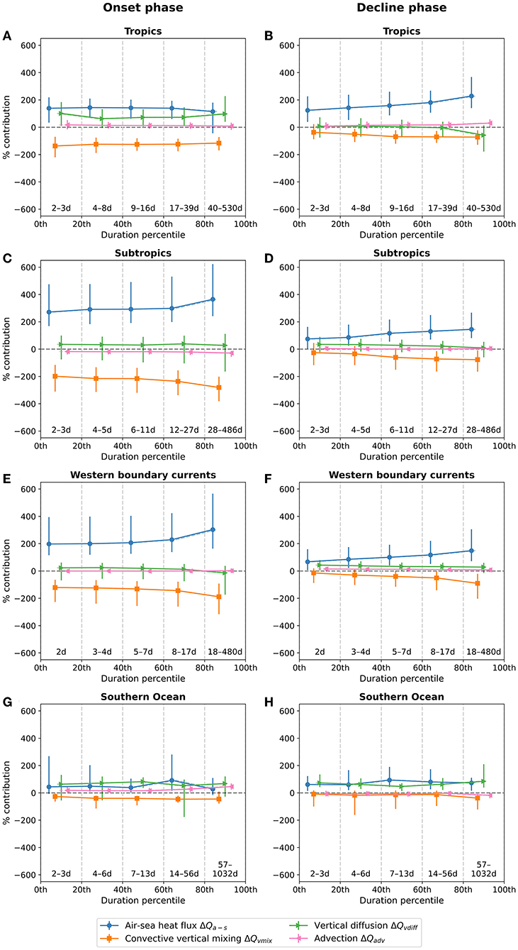
Figure 7. The dependence of the marine heatwave drivers on the duration of marine heatwaves in four selected regions. The panels show the percentage contribution of marine heatwave drivers to the full temperature tendency during the onset and decline phases for different durations (start-to-end) of marine heatwaves in the tropics (A,B), subtropics (C,D), western boundary currents (E,F), and Southern Ocean (G,H). Each point gives the median percentage contribution of a driver to the total temperature anomaly during marine heatwaves with a duration within 10 percentage points of the duration percentile indicated on the x-axis. The vertical error bars show the interquartile range. For visual clarity, points within each duration bin are separated by a small horizontal distance. The regions are defined in Figure 8.

Figure 7 also reveals the relatively large spread around each driver's median contribution. This large spread, shown by the interquartile range, indicates that different possible combinations of processes are possible for individual events, even at a similar duration. This spread is often largest for long MHW events. Even though air-sea heat flux anomalies are generally the main drivers for the onset and decline of MHWs, the balance of the different drivers is especially delicate during the decline of MHWs. The large spread indicates that MHWs can decline via many combinations of air-sea heat flux, vertical diffusion, and even convective vertical mixing anomalies. The Southern Ocean is the region with the smallest signal-to-noise ratio during both phases, meaning that diverse driver combinations are possible (Figures 7G,H). For example, the longest events in the Southern Ocean (longer than 57 days, the local 80th duration percentile) are driven by any of the four drivers and decline mostly via air-sea heat flux and vertical diffusion anomalies with possible contributions from the other two terms. The sign and median magnitude of each driver's contribution are more clear in the subtropics (Figures 7C,D) and western boundary current regions (Figures 7E,F). But even there, the relationship between drivers can differ from the mean picture. This is especially true for long events, where the ranges of possible driver contributions are large. For these events, we see that vertical diffusion during onset, as well as vertical diffusion and convective vertical mixing during decline, can be of either sign for different events and thus either support or inhibit the respective MHW phase. In the tropics during onset (Figure 7A), the air-sea heat flux and vertical diffusion contributions are of similar magnitude and events can be built up with either of the two drivers as the main contributor. One important source of this variability in MHW drivers among events that we observe in all regions may be the seasonality of the drivers (Figures 4–6).

3.4. Driver Classification of MHW Types

Given the many combinations of drivers that may lead to the onset and decline of MHWs, we use a K-Means clustering approach to classify different MHW types (see Section 2.5). Figure 8 shows the three MHWs types (1, 2, or 3) identified by the clustering algorithm in each region (i.e., Tropics, Subtrop—Subtropics, WBC—Western Boundary Currents, SouthOc—Southern Ocean). These regions represent distinct large-scale oceanographic features and are shown in Figure 8E. The figure also lists the percentage of MHWs and MHW days occupied by MHWs of each type, along with the median duration and median maximal magnitude of MHWs of each type. The MHW types identified by the clustering algorithm differ in their onset and decline drivers, both in magnitude and sometimes also in sign (Figure 8). Additionally, different types have different median durations, magnitudes, and locations of the peak in the calendar year (Supplementary Figure 4).

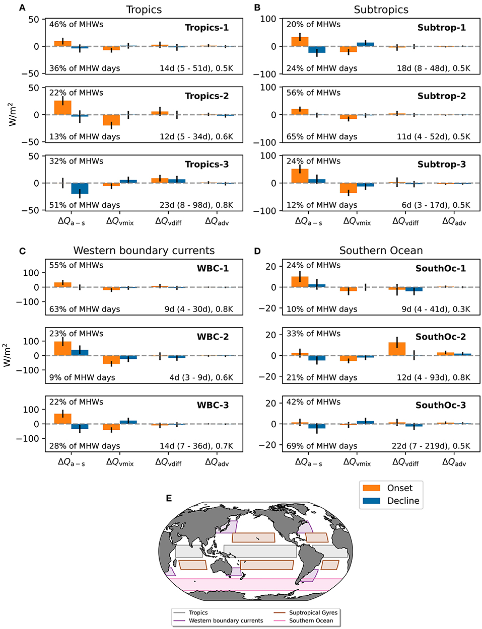
Figure 8. (A–D) Marine heatwave types identified by K-Means clustering in four selected regions. Error bars show the standard deviation of each driver's anomaly among marine heatwaves of each type. The median duration (in days), median maximal magnitude (in Kelvin) and the percentage of marine heatwaves and marine heatwave days occupied by marine heatwaves of each type are also given. Note the different y-axis scales used for different regions. The bottom panel (E) shows the definition of the regions. The definitions of the western boundary current regions are as in Hayashida et al. (2020), Figures 5, 6 therein.

In the tropics, there exist distinct types of main driving process combinations responsible for the MHW onset (Figure 8A). The first two MHW types (represented by Tropics-1 and Tropics-2) are built up by air-sea heat flux, with a small contribution from vertical diffusion and counteracting effects from convective vertical mixing, and decline mostly via air-sea heat flux. Tropics-1 and Tropics-2 have similar median durations and magnitudes, and differ from each other only in the magnitude but not in sign of each driver. The third MHW type in the tropics (Tropics-3) builds up heat via vertical diffusion. It declines via air-sea heat flux, which is counteracted by persistent positive vertical diffusion anomalies and by convective vertical mixing. This MHW type has the longest median duration and highest median magnitude in the tropics, and it occurs preferentially in December and January (Supplementary Figure 5). By applying the clustering procedure to each subregion separately (not shown), we find that the long and intense type Tropics-3 occurs almost exclusively in the tropical Pacific. This is linked to El Niño events, since 76% of MHW days in the tropics co-occur with El Niño events as defined using a 0.4 K threshold on the 5-month running mean SST anomaly in the Niño3.4 region (5N–5S, 170W–120W).

In the subtropics, the three identified MHW types are similar in their driver contributions, indicating similar MHW behavior in the subtropics even across ocean basins (Figure 8B). The onset phase is mainly driven by air-sea heat flux with counteracting effects from convective vertical mixing. The only substantial differences among the three types in the subtropics are found during the decline phase, where either convective vertical mixing (Subtrop-3) or air-sea heat flux (Subtrop-1) provide the main contribution. The median magnitude of 0.5 K is the same across all types. Note however that events can still differ among each other both qualitatively and quantitatively due to e.g., the seasonality of the drivers, as indicated by the error bars in Figure 8B.

A similar picture is found in the western boundary current regions, where the onset of MHWs is again mostly driven by air-sea heat flux in all three types, and decline is caused by either convective vertical mixing or air-sea heat flux (Figure 8C). However, we find additional contributions from vertical diffusion in type WBC-2, where it counteracts MHW onset and reinforces decline. During the onset, advection is only locally important (Figure 3K). The differences in median MHW magnitude across the three types is more pronounced compared to the subtropics.

In the Southern Ocean region, the three identified types differ substantially (Figure 8D). This is in line with the results in Figure 7, where the Southern Ocean is the region with the smallest signal-to-noise ratio in its typical driver balance, allowing for the existence of diverse MHW types. SouthOc-1 is built up by air-sea heat flux with counteracting anomalies from vertical diffusion and convective vertical mixing. SouthOc-2 represents an MHW type where the MHW onset is predominantly driven by vertical diffusion, with small contributions from all the other three terms. The type with the largest median duration in this region, SouthOc-3, is characterized by a balance of small contributions from all four drivers during both phases. The seasonality of these types is also remarkable (Supplementary Figure 4). All types have their peak preferentially in summer, and the type SouthOc-2, which is the only type globally which is predominantly driven by vertical diffusion, peaks almost exclusively in summer.

We also find that types are similar even across regions, even though no a priori relation exists between the types in different regions, since the algorithm was applied to each of the four regions separately. For example, a close similarity can be found between the different MHW types in the Subtropics and WBC regions: Subtrop-1 has similar driver contributions as WBC-3, Subtrop-2 as WBC-1, and Subtrop-3 as WBC-2. However, there also exist types which have no analogs in other regions, such as the types Tropics-3 and SouthOc-2.

4. Discussion and Conclusion

Our analysis shows that anomalous net ocean heat uptake is generally the most dominant driver of the onset (net uptake of heat from the atmosphere) and decline (net loss of heat to the atmosphere) of MHWs year-round. An exception is the equatorial Pacific, where the ocean takes up less heat than usual during both the onset and decline phase, but gains heat through an increase in convective vertical mixing and a reduction of vertical diffusion during the onset phase. The vertical diffusion term exhibits the largest seasonal variability for both the onset and decline phase. The total net air-sea heat flux anomaly does not show a large seasonality but its individual components, in particular shortwave radiation and latent heat fluxes, do show a distinct seasonal behavior. There is no strong relation between the duration of MHWs and the relative importance of their drivers, but there is in some regions an increased counteracting effect between air-sea heat flux and convective vertical mixing for longer events. Nevertheless, different MHWs with similar duration and even occurring in the same region can be driven by qualitatively and/or quantitatively distinct combinations of driving processes. These combinations can be interpreted as different MHW types, as represented by the clustering approach in this study. Whereas the types in the subtropics and the western boundary current regions differ mainly in driver magnitude, the types in the tropics and in the Southern Ocean exhibit marked qualitative differences in their drivers.

Although a detailed comparison with individual observed MHWs and their driving processes is difficult and partially hampered by the coarse resolution of the GFDL ESM2M model, especially for MHWs occurring in the western boundary current regions (Hayashida et al., 2020) or coastal regions (Guo et al., 2022), as well as by large differences in the drivers among individual events, our model results are in good agreement with previous findings for the open ocean. The predominance of atmospheric-driven MHWs in many regions is consistent with the observation-based synthesis of Holbrook et al. (2019) (Table 1 therein) and also with a number of MHW case studies which identified air-sea heat fluxes as a principal cause (Olita et al., 2007; Chen et al., 2014; Perkins-Kirkpatrick et al., 2019). For example, the onset of the high SSTs during the 'Blob' MHW in the Northeast Pacific during 2013/14 was associated with a persistent high pressure system including weaker winds, which caused lower than normal rates of heat loss from the ocean to the atmosphere (Bond et al., 2015; Gentemann et al., 2017). Similarly, the summer Northeast Pacific 2019 MHW was caused by reduced surface winds and associated reduced evaporative cooling and wind-driven upper ocean mixing. These warmer ocean conditions then reduced low-cloud fraction which reinforced the MHW onset through a positive low cloud feedback (i.e., increasing incoming shortwave radiation; Amaya et al., 2020). In our study, reduced latent heat loss and increased incoming shortwave radiation are also the main drivers of summer MHWs in these regions, and the model also simulates reduced wind stress and reduced cloud cover (Figure 4C). In addition, the combination of reduced wind stress and associated increased net air-sea heat fluxes into the ocean from increased insolation or decreased net latent and sensible heat fluxes was also seen during the Mediterranean Sea MHW in 2003 (Sparnocchia et al., 2006; Olita et al., 2007), the 2012 Northwest Atlantic MHW (Chen et al., 2014), and the 2017/2018 Tasman Sea MHW (Perkins-Kirkpatrick et al., 2019), as well as for marine heatwaves in the Indian Ocean (Saranya et al., 2022) and in general for the most extreme MHWs (Sen Gupta et al., 2020). This is consistent with our finding of increased air-sea heat flux during MHW onset and reduced wind stress over most of the global ocean (Figures 4A,C,E). It has been suggested that the onset periods of MHWs in the Northwest Atlantic are mainly atmospherically driven and decline proceeds more through oceanic processes (Schlegel et al., 2021). This suggestion can not be evaluated in great detail here due to the coarse model resolution that limits the model skill in this western boundary current region. However, our results confirm at the global scale that the MHW onset is predominantly driven by the atmosphere, and there exist types of MHWs that decline via oceanic processes in most regions. More generally, the existence of ocean-driven MHWs, which have been observed historically (e.g., Benthuysen et al., 2014; Sen Gupta et al., 2020) has been confirmed here with the clustering approach. MHWs are often associated with large-scale climate variability modes, such as the El Niño Southern Oscillation (ENSO), and teleconnections (Holbrook et al., 2019; Sen Gupta et al., 2020), as they can remotely modulate local driving processes of MHWs. For example, MHW occurrences in the eastern equatorial Pacific, central Indian Ocean as well as parts of the Southern Ocean and the eastern Atlantic basin are significantly related to ENSO (Holbrook et al., 2019). Subsequent studies should investigate how our identified local processes, especially vertical convective mixing and vertical diffusion, are modulated by such large-scale modes of variability.

It has been shown that the prevalent weather patterns of different seasons may lead to different kinds of driving forces depending on season (Amaya et al., 2020). Sen Gupta et al. (2020) show that the most intense MHWs tend to occur in summer, due to factors such as shallow mixed layer depths and weaker wind speeds, among others. We also find distinct seasonality in the magnitude (Supplementary Figure 5) and the drivers of MHWs (Figures 4–6), and our analysis similarly points to a connection between wind stress anomalies and MHW drivers such as latent heat flux as well as vertical diffusion and mixing (Sections 3.1 and 3.2). Furthermore, our cluster analysis shows that some MHW types preferentially occur in certain seasons over others (Supplementary Figure 4).

Even though we consider our conclusions to be robust, a number of caveats and the potential for subsequent work needs to be discussed, such as (i) the impact of model resolution, model and simulation selection, and (ii) the focus on surface marine heatwaves. First, we use a relatively coarse-resolution Earth system model. Recent studies suggest that such coarse-resolution models underestimate the magnitude of marine heatwaves, especially in western boundary currents, where the eddy-driven mesoscale circulation is crucial for driving high temperatures extremes (Pilo et al., 2019; Hayashida et al., 2020). We find that in western boundary currents, all of the four most dominant processes, such as air-sea heat flux, convective vertical mixing, vertical diffusion and advection, are involved in the onset and decline of marine heatwaves. However, due to the lack of eddy-driven variability in our coarse resolution model, these results should be viewed with caution. For instance, we only find a strong horizontal and vertical advective signal in the Northern Hemisphere western boundary currents (Figure 3), but advection may also play a role in the Southern Hemisphere western boundary currents (Oliver et al., 2017). Furthermore, the identified MHW types in the western boundary currents may show too large contributions from air-sea heat flux in relation to advection (Figure 8C, type WBC-2). In addition, we only use one single model and therefore such analyses should be repeated with other models. We also focus on a preindustrial simulation without anthropogenic influence. However, our main results are well reproduced using present-day forcing for the same model (Supplementary Figure 2). The robustness of our findings concerning the dependence of MHW drivers on event duration (Section 3.3) should be further investigated in subsequent studies, since an analogous analysis has not yet been done using observational data.

Second, our present analysis considered processes only at the sea surface. However, our analysis framework could be extended to include extreme events and their driving mechanisms below the surface, where the acting processes may be very different (Elzahaby and Schaeffer, 2019). An analysis of the most important drivers at the subsurface in our model is shown in Supplementary Figure 6. It suggests that it is in fact horizontal and vertical advection which dominates the onset and decline of MHWs at 95m depth in the annual mean, especially in low latitudes. However, a comparison with observation-based data would be even more difficult at subsurface, because of the current lack of observations.

In summary, our preindustrial GFDL ESM2M simulation suggests that the onset of MHWs is mainly driven by air-sea heat uptake at local scale due to a decrease in latent heat loss, especially in the subtropics and mid-to-high latitudes. However, individual MHWs can be caused by a combination of different drivers, especially in the Southern Ocean and the tropical ocean, and driving processes can vary seasonally. Our results imply that detailed knowledge of oceanic heat budget processes is vital for a complete understanding of marine heatwave dynamics and may aid in the prediction and attribution of marine heatwaves in the future.

Data Availability Statement

The datasets and code required to reproduce the figures and tables in this study can be found at: https://doi.org/10.5281/zenodo.6384637.

Author Contributions

LV, FB, and TF conceived the study. The preindustrial simulation was conducted by FB. SG led the implementation of the temperature tendency terms in GFDL ESM2M. LV did the analysis, produced the figures, and wrote the initial draft. All authors helped with interpretation and contributed to the writing. All authors contributed to the article and approved the submitted version.

Funding

This research has been supported by the Swiss National Science Foundation (grant no. PP00P2_198897) and the European Union's Horizon 2020 research and innovative program under grant agreement no. 820989 (project COMFORT), our common future ocean in the Earth system–quantifying coupled cycles of carbon, oxygen, and nutrients for determining and achieving safe operating spaces with respect to tipping points (grant no. 820989), and grant agreement no. 862923 (project AtlantECO, Atlantic Ecosystems Assessment, Forecasting & Sustainability). The model simulation has been conducted at the Swiss National Supercomputing Centre (CSCS).

Conflict of Interest

The authors declare that the research was conducted in the absence of any commercial or financial relationships that could be construed as a potential conflict of interest.

Publisher's Note

All claims expressed in this article are solely those of the authors and do not necessarily represent those of their affiliated organizations, or those of the publisher, the editors and the reviewers. Any product that may be evaluated in this article, or claim that may be made by its manufacturer, is not guaranteed or endorsed by the publisher.

Acknowledgments

The authors thank Jamie Palter for a helpful discussion about the interpretation of the GFDL ESM2M temperature tendency terms, and Rick Slater and Jasmin John for help with the implementation of the tendency terms into GFDL ESM2M. We thank Anne Morée for comments on an earlier draft of the manuscript.

Supplementary Material

The Supplementary Material for this article can be found online at: https://www.frontiersin.org/articles/10.3389/fclim.2022.847995/full#supplementary-material

References

Amaya, D. J., Miller, A. J., Xie, S.-P., and Kosaka, Y. (2020). Physical drivers of the summer 2019 North Pacific marine heatwave. Nat. Commun. 11, 1903. doi: 10.1038/s41467-020-15820-w
Anderson, J. L., The GFDL Global Atmospheric Model Development Team, Balaji, V., Broccoli, A. J., Cooke, W. F., Delworth, T. L., and Dixon, K. W. (2004). The New GFDL Global Atmosphere and Land Model AM2–LM2: evaluation with prescribed SST simulations. J. Clim. 17, 4641–4673. doi: 10.1175/JCLI-3223.1
Babcock, R. C., Bustamante, R. H., Fulton, E. A., Fulton, D. J., Haywood, M. D. E., Hobday, A. J., et al. (2019). Severe continental-scale impacts of climate change are happening now: extreme climate events impact marine habitat forming communities along 45% of Australia's Coast. Front. Mar. Sci. 6, 411. doi: 10.3389/fmars.2019.00411
Bensoussan, N., Romano, J.-C., Harmelin, J.-G., and Garrabou, J. (2010). High resolution characterization of northwest Mediterranean coastal waters thermal regimes: to better understand responses of benthic communities to climate change. Estuar. Coast. Shelf Sci. 87, 431–441. doi: 10.1016/j.ecss.2010.01.008
Benthuysen, J., Feng, M., and Zhong, L. (2014). Spatial patterns of warming off Western Australia during the 2011 Ningaloo Niño: quantifying impacts of remote and local forcing. Continent. Shelf Res. 91, 232–246. doi: 10.1016/j.csr.2014.09.014
Bond, N. A., Cronin, M. F., Freeland, H., and Mantua, N. (2015). Causes and impacts of the 2014 warm anomaly in the NE Pacific. Geophys. Res. Lett. 42, 3414–3420. doi: 10.1002/2015GL063306
Bopp, L., Resplandy, L., Orr, J. C., Doney, S. C., Dunne, J. P., Gehlen, M., et al. (2013). Multiple stressors of ocean ecosystems in the 21st century: projections with CMIP5 models. Biogeosciences 10, 6225–6245. doi: 10.5194/bg-10-6225-2013
Burger, F. A., John, J. G., and Frölicher, T. L. (2020). Increase in ocean acidity variability and extremes under increasing atmospheric CO2. Biogeosciences 17, 4633–4662. doi: 10.5194/bg-17-4633-2020
Chen, K., Gawarkiewicz, G. G., Lentz, S. J., and Bane, J. M. (2014). Diagnosing the warming of the Northeastern U.S. Coastal Ocean in 2012: a linkage between the atmospheric jet stream variability and ocean response. J. Geophys. Res. Oceans 119, 218–227. doi: 10.1002/2013JC009393
Cheung, W. W. L., and Frölicher, T. L. (2020). Marine heatwaves exacerbate climate change impacts for fisheries in the northeast Pacific. Sci. Rep. 10, 6678. doi: 10.1038/s41598-020-63650-z
Cheung, W. W. L., Frölicher, T. L., Lam, V. W. Y., Oyinlola, M. A., Reygondeau, G., Sumaila, U. R., et al. (2021). Marine high temperature extremes amplify the impacts of climate change on fish and fisheries. Sci. Adv. 7, eabh0895. doi: 10.1126/sciadv.abh0895
Collins, M., Sutherland, L., Bouwer, L., Cheong, S.-M., Frölicher, T., et al. (2019). “Extremes, abrupt changes and managing risks,” in IPCC Special Report on the Ocean and Cryosphere in a Changing Climate, eds H.-O. Pörtner, D. C. Roberts, V. Masson-Delmotte, P. Zhai, M. Tignor, E. Poloczanska, K. Mintenbeck, A. Alegría, M. Nicolai, A. Okem, J. Petzold, B. Rama, and N. M. Weyer (Cambridge; New York, NY: Cambridge University Press), 589–655. doi: 10.1017/9781009157964.008
Di Lorenzo, E., and Mantua, N. (2016). Multi-year persistence of the 2014/15 North Pacific marine heatwave. Nat. Clim. Change 6, 1042–1047. doi: 10.1038/nclimate3082
Dunne, J. P., John, J. G., Adcroft, A. J., Griffies, S. M., Hallberg, R. W., Shevliakova, E., et al. (2012). GFDL's ESM2 global coupled climate–carbon earth system models. Part I: physical formulation and baseline simulation characteristics. J. Clim. 25, 6646–6665. doi: 10.1175/JCLI-D-11-00560.1
Dunne, J. P., John, J. G., Shevliakova, E., Stouffer, R. J., Krasting, J. P., Malyshev, S. L., et al. (2013). GFDL's ESM2 global coupled climate–carbon earth system models. Part II: carbon system formulation and baseline simulation characteristics. J. Clim. 26, 2247–2267. doi: 10.1175/JCLI-D-12-00150.1
Echevin, V., Colas, F., Espinoza-Morriberon, D., Vasquez, L., Anculle, T., and Gutierrez, D. (2018). Forcings and evolution of the 2017 coastal El Niño off Northern Peru and Ecuador. Front. Mar. Sci. 5, 367. doi: 10.3389/fmars.2018.00367
Elzahaby, Y., and Schaeffer, A. (2019). Observational insight into the subsurface anomalies of marine heatwaves. Front. Mar. Sci. 6, 745. doi: 10.3389/fmars.2019.00745
Feng, M., McPhaden, M. J., Xie, S.-P., and Hafner, J. (2013). La Niña forces unprecedented Leeuwin Current warming in 2011. Sci. Rep. 3, 1277. doi: 10.1038/srep01277
Filbee-Dexter, K., and Wernberg, T. (2018). Rise of turfs: a new battlefront for globally declining kelp forests. Bioscience 68, 64–76. doi: 10.1093/biosci/bix147
Fox-Kemper, B., Ferrari, R., and Hallberg, R. (2008). Parameterization of mixed layer Eddies. Part I: theory and diagnosis. J. Phys. Oceanogr. 38, 1145–1165. doi: 10.1175/2007JPO3792.1
Frölicher, T. L., Fischer, E. M., and Gruber, N. (2018). Marine heatwaves under global warming. Nature 560, 360–364. doi: 10.1038/s41586-018-0383-9
Frölicher, T. L., and Laufkötter, C. (2018). Emerging risks from marine heat waves. Nat. Commun. 9, 650. doi: 10.1038/s41467-018-03163-6
Gentemann, C. L., Fewings, M. R., and García-Reyes, M. (2017). Satellite sea surface temperatures along the West Coast of the United States during the 2014-2016 northeast Pacific marine heat wave: Coastal SSTs During “the Blob”. Geophys. Res. Lett. 44, 312–319. doi: 10.1002/2016GL071039
Griffies, S. (1998). The Gent–McWilliams Skew Flux. J. Phys. Oceanogr. 28, 831–841. doi: 10.1175/1520-0485(1998)028<0831:TGMSF>2.0.CO;2
Griffies, S. M. (2012). Elements of the Modular Ocean Model (MOM). Available online at: https://mom-ocean.github.io/assets/pdfs/MOM5_manual.pdf (accessed December 1, 2021).
Griffies, S. M. (2015). Working Notes on the Ocean Heat Budget in GFDL-ESM2M. Available online at: https://mom-ocean.github.io/assets/pdfs/ESM2M_heat_budget.pdf (accessed December 1, 2021).
Griffies, S. M., Danabasoglu, G., Durack, P. J., Adcroft, A. J., Balaji, V., Böning, C. W., et al. (2016). OMIP contribution to CMIP6: experimental and diagnostic protocol for the physical component of the Ocean Model Intercomparison Project. Geosci. Model Dev. 9, 3231–3296. doi: 10.5194/gmd-9-3231-2016
Griffies, S. M., and Greatbatch, R. J. (2012). Physical processes that impact the evolution of global mean sea level in ocean climate models. Ocean Modell. 51, 37–72. doi: 10.1016/j.ocemod.2012.04.003
Griffies, S. M., Winton, M., Anderson, W. G., Benson, R., Delworth, T. L., Dufour, C. O., et al. (2015). Impacts on ocean heat from transient mesoscale Eddies in a hierarchy of climate models. J. Clim. 28, 952–977. doi: 10.1175/JCLI-D-14-00353.1
Griffies, S. (2009). Elements of MOM4p1. Available online at: https://mom-ocean.github.io/assets/pdfs/MOM4p1_manual.pdf (accessed December 1, 2021).
Gruber, N., Boyd, P. W., Frölicher, T. L., and Vogt, M. (2021). Biogeochemical extremes and compound events in the ocean. Nature 600, 395–407. doi: 10.1038/s41586-021-03981-7
Guo, X., Gao, Y., Zhang, S., Wu, L., Chang, P., Cai, W., et al. (2022). Threat by marine heatwaves to adaptive large marine ecosystems in an Eddy-resolving model. Nat. Clim. Change 12, 179–186. doi: 10.1038/s41558-021-01266-5
Hayashida, H., Matear, R. J., Strutton, P. G., and Zhang, X. (2020). Insights into projected changes in marine heatwaves from a high-resolution ocean circulation model. Nat. Commun. 11, 4352. doi: 10.1038/s41467-020-18241-x
Hobday, A. J., Alexander, L. V., Perkins, S. E., Smale, D. A., Straub, S. C., Oliver, E. C. J., et al. (2016). A hierarchical approach to defining marine heatwaves. Prog. Oceanogr. 141, 227–238. doi: 10.1016/j.pocean.2015.12.014
Holbrook, N. J., Scannell, H. A., Sen Gupta, A., Benthuysen, J. A., Feng, M., Oliver, E. C. J., et al. (2019). A global assessment of marine heatwaves and their drivers. Nat. Commun. 10, 2624. doi: 10.1038/s41467-019-10206-z
Huang, B., Liu, C., Banzon, V., Freeman, E., Graham, G., Hankins, B., et al. (2020). Improvements of the daily optimum interpolation sea surface temperature (DOISST) Version 2.1. J. Clim. 34, 1–47. doi: 10.1175/JCLI-D-20-0166.1
Hughes, T. P., Kerry, J. T., Álvarez-Noriega, M., Álvarez-Romero, J. G., Anderson, K. D., Baird, A. H., et al. (2017). Global warming and recurrent mass bleaching of corals. Nature 543, 373–377. doi: 10.1038/nature21707
IPCC (2019). “Glossary,” in IPCC Special Report on the Ocean and Cryosphere in a Changing Climate, ed N. Weyer (IPCC).
Jacox, M. G., Alexander, M. A., Bograd, S. J., and Scott, J. D. (2020). Thermal displacement by marine heatwaves. Nature 584, 82–86. doi: 10.1038/s41586-020-2534-z
James, G., Witten, D., Hastie, T., and Tibshirani, R. (2014). “Unsupervised learning,” An Introduction to Statistical Learning: With Applications in R (New York, NY: Springer), 373–418. doi: 10.1007/978-1-4614-7138-7_10
Large, W. G., McWilliams, J. C., and Doney, S. C. (1994). Oceanic vertical mixing: a review and a model with a nonlocal boundary layer parameterization. Rev. Geophys. 32, 363–403. doi: 10.1029/94RG01872
Laufkötter, C., Zscheischler, J., and Frölicher, T. L. (2020). High-impact marine heatwaves attributable to human-induced global warming. Science 369, 1621–1625. doi: 10.1126/science.aba0690
Manizza, M., Le Quéré, C., Watson, A. J., and Buitenhuis, E. T. (2005). Bio-optical feedbacks among phytoplankton, upper ocean physics and sea-ice in a global model. Geophys. Res. Lett. 32, 5. doi: 10.1029/2004GL020778
Manta, G., de Mello, S., Trinchin, R., Badagian, J., and Barreiro, M. (2018). The 2017 record marine heatwave in the southwestern Atlantic Shelf. Geophys. Res. Lett. 45, 12,449–12,456. doi: 10.1029/2018GL081070
Martin, T., and Adcroft, A. (2010). Parameterizing the fresh-water flux from land ice to ocean with interactive icebergs in a coupled climate model. Ocean Modell. 34, 111–124. doi: 10.1016/j.ocemod.2010.05.001
Milly, P. C. D., Malyshev, S. L., Shevliakova, E., Dunne, K. A., Findell, K. L., Gleeson, T., et al. (2014). An enhanced model of land water and energy for global hydrologic and earth-system studies. J. Hydrometeorol. 15, 1739–1761. doi: 10.1175/JHM-D-13-0162.1
Olita, A., Sorgente, R., Natale, S., Gaberšek, S., Ribotti, A., Bonanno, A., et al. (2007). Effects of the 2003 European heatwave on the Central Mediterranean Sea: Surface fluxes and the dynamical response. Ocean Sci. 3, 273–289. doi: 10.5194/os-3-273-2007
Oliver, E. C. J. (2019). Mean warming not variability drives marine heatwave trends. Clim. Dyn. 53, 1653–1659. doi: 10.1007/s00382-019-04707-2
Oliver, E. C. J., Benthuysen, J. A., Bindoff, N. L., Hobday, A. J., Holbrook, N. J., Mundy, C. N., et al. (2017). The unprecedented 2015/16 Tasman Sea marine heatwave. Nat. Commun. 8, 16101. doi: 10.1038/ncomms16101
Oliver, E. C. J., Benthuysen, J. A., Darmaraki, S., Donat, M. G., Hobday, A. J., Holbrook, N. J., et al. (2021). Marine heatwaves. Annu. Rev. Mar. Sci. 13, 313–342. doi: 10.1146/annurev-marine-032720-095144
Oliver, E. C. J., Donat, M. G., Burrows, M. T., Moore, P. J., Smale, D. A., Alexander, L. V., et al. (2018). Longer and more frequent marine heatwaves over the past century. Nat. Commun. 9, 1324. doi: 10.1038/s41467-018-03732-9
Palter, J. B., Frölicher, T. L., Paynter, D., and John, J. G. (2018). Climate, ocean circulation, and sea level changes under stabilization and overshoot pathways to 1.5 K warming. Earth Syst. Dyn. 9, 817–828. doi: 10.5194/esd-9-817-2018
Palter, J. B., Griffies, S. M., Samuels, B. L., Galbraith, E. D., Gnanadesikan, A., and Klocker, A. (2014). The deep ocean buoyancy budget and its temporal variability. J. Clim. 27, 551–573. doi: 10.1175/JCLI-D-13-00016.1
Perkins-Kirkpatrick, S. E., King, A. D., Cougnon, E. A., Holbrook, N. J., Grose, M. R., Oliver, E. C. J., et al. (2019). The role of natural variability and anthropogenic climate change in the 2017/18 Tasman Sea marine heatwave. Bull. Am. Meteorol. Soc. 100, S105–S110. doi: 10.1175/BAMS-D-18-0116.1
Pilo, G. S., Holbrook, N. J., Kiss, A. E., and Hogg, A. M. (2019). Sensitivity of marine heatwave metrics to ocean model resolution. Geophys. Res. Lett. 46, 14604–14612. doi: 10.1029/2019GL084928
Plecha, S. M., and Soares, P. M. M. (2020). Global marine heatwave events using the new CMIP6 multi-model ensemble: from shortcomings in present climate to future projections. Environ. Res. Lett. 15, 124058. doi: 10.1088/1748-9326/abc847
Rodrigues, R. R., Taschetto, A. S., Sen Gupta, A., and Foltz, G. R. (2019). Common cause for severe droughts in South America and marine heatwaves in the South Atlantic. Nat. Geosci. 12, 620–626. doi: 10.1038/s41561-019-0393-8
Saranya, J. S., Roxy, M. K., Dasgupta, P., and Anand, A. (2022). Genesis and trends in marine heatwaves over the tropical Indian Ocean and their interaction with the Indian summer monsoon. J. Geophys. Res. Oceans 127, e2021JC017427. doi: 10.1029/2021JC017427
Schlegel, R. W., Oliver, E. C. J., and Chen, K. (2021). Drivers of marine heatwaves in the Northwest Atlantic: the role of air–sea interaction during onset and decline. Front. Mar. Sci. 8, 627970. doi: 10.3389/fmars.2021.627970
Schlegel, R. W., Oliver, E. C. J., Hobday, A. J., and Smit, A. J. (2019). Detecting marine heatwaves with sub-optimal data. Front. Mar. Sci. 6, 737. doi: 10.3389/fmars.2019.00737
Schlegel, R. W., Oliver, E. C. J., Perkins-Kirkpatrick, S., Kruger, A., and Smit, A. J. (2017). Predominant atmospheric and oceanic patterns during coastal marine heatwaves. Front. Mar. Sci. 4, 323. doi: 10.3389/fmars.2017.00323
Sen Gupta, A., Thomsen, M., Benthuysen, J. A., Hobday, A. J., Oliver, E., Alexander, L. V., et al. (2020). Drivers and impacts of the most extreme marine heatwaves events. Sci. Rep. 10, 19359. doi: 10.1038/s41598-020-75445-3
Smale, D. A., Wernberg, T., Oliver, E. C. J., Thomsen, M., Harvey, B. P., Straub, S. C., et al. (2019). Marine heatwaves threaten global biodiversity and the provision of ecosystem services. Nat. Clim. Change 9, 306–312. doi: 10.1038/s41558-019-0412-1
Sparnocchia, S., Schiano, M. E., Picco, P., Bozzano, R., and Cappelletti, A. (2006). The anomalous warming of summer 2003 in the surface layer of the Central Ligurian Sea (Western Mediterranean). Ann. Geophys. 24, 443–452. doi: 10.5194/angeo-24-443-2006
Suarez-Gutierrez, L., Milinski, S., and Maher, N. (2021). Exploiting large ensembles for a better yet simpler climate model evaluation. Clim. Dyn. 57, 2557–2580. doi: 10.1007/s00382-021-05821-w
Wernberg, T., Russell, B. D., Thomsen, M. S., Gurgel, C. F. D., Bradshaw, C. J. A., Poloczanska, E. S., et al. (2011). Seaweed communities in retreat from ocean warming. Curr. Biol. 21, 1828–1832. doi: 10.1016/j.cub.2011.09.028
Keywords: marine heatwave, local drivers, extreme events, Earth system model, ocean heat budget
Citation: Vogt L, Burger FA, Griffies SM and Frölicher TL (2022) Local Drivers of Marine Heatwaves: A Global Analysis With an Earth System Model. Front. Clim. 4:847995. doi: 10.3389/fclim.2022.847995
Received: 03 January 2022; Accepted: 14 March 2022;
Published: 03 May 2022.
Edited by:
Alex Sen Gupta, University of New South Wales, AustraliaReviewed by:
Andrea Taschetto, University of New South Wales, AustraliaRobert William Schlegel, Institut de la Mer de Villefranche (IMEV), France
Copyright © 2022 Vogt, Burger, Griffies and Frölicher. This is an open-access article distributed under the terms of the Creative Commons Attribution License (CC BY). The use, distribution or reproduction in other forums is permitted, provided the original author(s) and the copyright owner(s) are credited and that the original publication in this journal is cited, in accordance with accepted academic practice. No use, distribution or reproduction is permitted which does not comply with these terms.
*Correspondence: Linus Vogt, linus.vogt@locean.ipsl.fr
†Present address: Linus Vogt, Sorbonne Université, LOCEAN-IPSL, Paris, France