Predictive Statistical Cost Estimation Model for Existing Single Family Home Elevation Projects

Introduction

Elevating the lowest floor of existing homes is widely considered to be the most effective building-scale flood mitigation strategy (Bellomo et al., 1999; FEMA 2010; FEMA 2012; Li and van De Lindt 2012; Bohn 2013), in contrast to acquisition and reconstruction. In spite of the effectiveness of elevation, this construction technique is performed by highly specialized contractors and generalized cost guidance is not widely available. At the project decision stage, benefit-cost analysis (BCA) must demonstrate a positive return on investment (FEMA 2011; Orooji and Friedland 2017). Thus, reasonable cost estimates are needed for comparison with long-term benefits to evaluate the most economically efficient strategies to achieve overall mitigation goals and provide economic justification for specific projects (Renn, 1998; Amoroso and Fennell 2008).

Conventional methods for project cost estimation are unit-cost and unit-area-cost. Unit-cost is project-specific, with exact construction quantities and historical unit-price costs, while unit-area-cost is based on general building attributes such as occupancy, building type, and other building parameters. In the absence of proprietary historical cost data, RSMeans (Waier and Balboni 2018) is commonly used to estimate construction cost. However, RSMeans data do not include all necessary construction activities for elevation projects and prices can vary substantially by contractor (Gair et al., 2011). These and similar shortcomings limit the ability of stakeholders (e.g., federal, state, and local agencies, homeowners) to estimate elevation project cost effectively.

Acknowledging this issue, elevation cost guidance has been developed previously. USACE (1993) reported that for a 0.6 m (2 foot) elevation, elevating wood-frame buildings with existing pile, post, or pier foundations costs $280/m² ($26/ft²), while elevating slab buildings costs $320/m² ($30/ft²) in 1993 dollars. Considering a 140 m² (1,500 ft²) house with 0.6-m (2-ft) elevation, additional costs associated with earthen fill (slab only), landscaping, engineering design, and contract cost bring these values to $380/m² ($35/ft²) for pile, post, or pier foundations and $450/m² ($42/ft²) for slab foundations in 1993 dollars. FEMA (1998) reported that for a 0.6- m (2-ft) elevation, elevating frame buildings with existing basement or crawl-space foundations onto continuous foundation walls or open foundations costs $180/m² ($17/ft²) while elevating frame or masonry slab buildings costs $510/m² ($47/ft²) in 1999 dollars. Newer guidance has moved away from providing elevation costs, as FEMA (2012) indicates that elevation cost relates to the type of construction and existing foundation but does not provide monetary values. In each of these documents, only mean cost values are reported, limiting consideration of the distribution of cost data. Most importantly, the effect of number of stories on elevation project cost is not mentioned in existing guidance. Thus, it is clear that updated cost guidance for existing home elevation projects is needed.

Predictive statistical cost modeling has been used in several construction cost applications (e.g., Herbsman 1986; Adeli and Wu 1998; Wilmot and Mei 2005), although not specific to home elevations. To predict construction cost, Karshenas (1984) used multiple regression, Skitmore and Ng (2003) used regression and cross-validation regression, and Kouskoulas and Koehn (1974) used multiple linear regression and validated the results with two real building case studies. Lowe et al (2006) used multiple linear regression, Jrade and Alkass (2007) developed a set of linear regression models in a computer-based cost estimation program, and Sonmez (2008) used a combination of linear regression and bootstrap techniques for construction cost modeling. Additionally, Shimizu et al. (2014) used switching regression model and generalized additive model (GAM) to predict the housing price, and Liu et al. (2018) used random forest and GAM to predict construction productivity using environmental factors. Specific to natural hazard mitigation, Jafarzadeh et al (2015) applied multiple linear regression to establish construction cost models for seismic retrofit of confined masonry buildings. Although statistical cost prediction models have been used for highways, commercial buildings, residential homes, and seismic retrofits, there are no known studies for existing building elevation cost prediction.

Conventional cost estimation methods are not readily accessible to decision-makers, and existing elevation cost guidance is limited and dated. Therefore, the goal of this paper is to evaluate and improve generalized home elevation construction cost estimation using predictive statistical modeling. This is accomplished by developing a robust, generalized cost estimation method for existing home elevations. Historical home elevation cost data obtained from the Louisiana Governor's Office of Homeland Security and Emergency Preparedness (GOHSEP) are categorized statistically using 10 regression models, a random forest model, and five GAMs with 10-fold cross-validation (CV) RMSE on all tested models. The required assumptions for each model are tested and the model with minimum prediction error is selected. Prediction results are compared with costs from USACE (1993), FEMA (1998), and Gair et al (2011) after modifying and updating them for time and location.

Both the methodology and the findings from the statistical model results are contributions of this research. First, previous statistical cost prediction research has evaluated limited models such as few regressions or GAMs; however, the method proposed in this research evaluates results from three robust statistical techniques, and external prediction accuracy of the selected models are examined. Second, the results themselves offer guidance to predict home elevation costs which enhance the flood mitigation decision-making and BCA (Taghinezhad et al., 2020a). Although the model results are applicable to Louisiana, the methodology itself can be applied for elevation mitigation project cost in other construction markets. Also, if the predicted elevation costs are adjusted for time and location, they may be representative of costs expected for similar buildings in similar construction markets.

Background

Elevation project cost varies based on several factors [Eq. 1], where C is the cost of the elevation project ($), A is the average floor area (m²) calculated as the total home area divided by the number of stories, ΔE is the change in first-floor elevation (FFE, m) calculated using Eq. 2, S is the number of stories, and F is a categorical variable representing foundation type. The FFE elevation (NAVD88) represents the top of the lowest floor (including basement, crawl-space, or enclosure floor) from elevation certificates, where FFE₀ and FFE₁ represent the FFE before and after elevation, respectively.

Data

Elevation Cost Literature

USACE (1993) calculates total cost of elevation ($C_t$; Eq. 3), where $C_e$ is the cost of elevation; $C_l$ represents the cost of landscaping excluding trees, bushes, and flowers; $C_p$ is the cost of professional engineering, and $P_c$ is the contract profit percentage. Landscaping cost ($C_l$) is calculated using Eqs. 4, 5, where $A_l$ represents the landscaping area, $C_{ul}$ represents the unit area landscaping cost, and $W_b$ and $L_b$ are the width and length of the building, respectively.

According to USACE (1993) the cost elevation values for 0.6 m (2ft) additional elevation are as: The C_e for “wood frame building on piles, posts or piers,” “wood frame building on foundation walls” “brick building,” and “slab-on-grade building” are $280/m² ($26/sf²), $205/m² ($19/sf²), $344/m² ($32/sf²), and $323/m² ($30/sf²), respectively. The C_ul, C_p, P_c, and earthen fill are $6/m² ($5/yd²), $7,000, 10%, $13/m3 ($10/yd3), respectively. The slab foundation is assumed to be converted to elevated foundations; however, cost values for earthen fill are also provided. Also, it must be noted that values provided in USACE (1993) are assumed to represent 1993 dollars.

FEMA (1998) simply provides unit costs to elevate existing buildings to continuous foundation walls or open foundations by 0.6 m (2ft) of $510/m² ($47/ft²) for frame or masonry buildings on slab foundations and $180/m² ($17/ft²) for frame buildings with basement or crawlspace foundation, assuming 1998 costs.

Gair et al. (2011) evaluated elevation cost for typical 140 m² (1,500ft²) one-story homes in Louisiana using unit-cost estimation and 2011 RSMeans residential cost data for slab and pier and beam foundations, elevated by 0.9 m (3ft), 1.8 m (6ft), and 2.7 m (9ft). However, because standard RSMeans cost data do not cover all construction activities required to elevate homes, Gair et al (2011) obtained unit cost values from a survey of foundation elevation contractors. Gair et al. (2011) divided the elevation process into 12 typical activities for Louisiana: push piling; raise, shore and align; footings; piers; wood stair; sanitary sewer; water; electrical; driveway and sidewalk pavement; platform for air conditioning (AC); remove/replace AC; and insulation below floor framing (per and beam only). Three additional activities are not typical for Louisiana: exterior wall; masonry stair; gas. The average cost/unit area/unit elevation for these three additional activities according to Gair et al. (2011) are 65.6 (1.9), 43.3 (1.2), and 9.0 (0.3), $ m⁻² m⁻¹ ($ ft⁻² ft⁻¹), respectively.

Cost Adjustment

Cost information from the literature was normalized to represent 2015 dollars using the Engineering News-Record (ENR) average annual building cost index (i.e., average index, AI; (Grogan, 2016), which is commonly used by researchers in the construction industry (e.g., Popescu et al., 2003; Touran and Lopez 2006; Mikhed and Zemčík 2009). AI values have been determined considering nationwide changes (i.e., 20 cities) in labor rates, productivity, material prices, and the competitive condition of the building marketplace. The AI values (Grogan, 2016) are used to calculate project cost in terms of 2015 dollars [Eq. 6], where C₂₀₁₅ is cost in 2015, AI₂₀₁₅ is the average index of the construction cost in 2015, AI_i is the average index at time i, and C_i represents cost at time i (i.e., either project contract date or year of previous study),. Historical AI values used for 1993, 1998, 2005, and 2015 are 2,996, 3,391, 4,205, and 5,517, respectively.

National average project costs ($C_{NA}$) were adjusted to represent Louisiana costs ($C_{LA}$) using average location factor, $P_l$ [Eq. 7], determined by averaging all Louisiana city RSMeans location factors (RSMeans, 2015). These factors ranged between 77.8 and 87.5%, with an average of 82.6%. Summarized costs are provided along with the results of this paper in Table 1

TABLE 1. Elevation cost (cost/unit area) comparison between model 5 m and cost guidance, $/m² ($/ft²).

Louisiana Elevation Project Data

Data were collected from scanned GOHSEP documents, corresponding to single-family homes elevated after major hurricane and flood events from 15 parishes (counties) in southern Louisiana between 2005 and 2015. Of the 805 total building records evaluated, the 666 with missing or spurious data were discarded from further analysis, thereby leaving 139 projects for statistical analysis. All cost data were adjusted to 2015 dollars, using the contract date as the original cost basis.

Seventy-one percent (71%) of the buildings had elevation certificates, from which elevation data were obtained. For the remaining buildings, FFE was obtained from other related building documents rather than the elevation certificate. The FFE in these documents was assumed to be the top of bottom floor (including basement, crawl-space, or enclosure floor) as specified in the elevation certificates.

Statistical summarization of variables used in the prediction model (Table 2) includes mean elevation cost per average floor area per unit ΔE ($825/m²/m), with a median of $821/m²/m, standard deviation of $425/m²/m, and range from $203/m²/m to $2,151/m²/m.

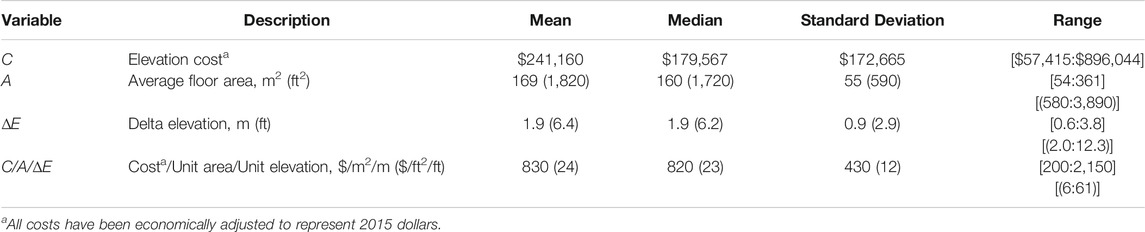
TABLE 2. Statistical mean, median, standard deviation and range for 139 observations.

The correlation matrix and boxplot for each variable enhance the understanding of collected data. The correlation matrix (Table 3) reveals the dependence between variables before statistical analysis. Cost correlates most strongly with number of stories, followed by ∆E. The elevation project cost boxplot shows many (13 out of 139) outliers above $500,000 (Figure 1). Data were weighted toward smaller values, which in turn indicates that the majority of collected data are associated with small and medium-sized homes. However, some outliers appear at the upper tail of the average floor area distribution. The ΔE boxplot shows that 67 out of 139 buildings (48%) were elevated in the range of 1.1 m (3.6 ft.) to 2.7 m (8.9ft). Data for ΔE data are slightly right-skewed but are normally distributed along the available range of elevation data.

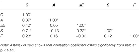
TABLE 3. Correlation matrix for independent variables in sampled elevated homes in Louisiana, 2005–2015.

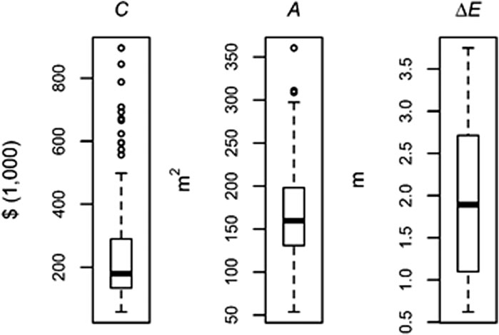
FIGURE 1. Boxplots of continuous variables for elevated homes in Louisiana, 2005–2015, cost normalized to 2015 dollars.

Of the 139 elevation projects, 105 buildings are one-story, while 34 buildings are two-story. Four initial foundation types exist in the data: slab (116), crawl-space (2), pier and beam (15), and piling (6). Since there were only two levels of building stories in the data set, this variable was converted to a categorical variable with levels 0 and 1, representing one- and two-story buildings, respectively. In addition, slab foundations were the most predominant foundation type, with only 23 observations of other foundation types. Thus, the foundation type variable was also converted to a categorical variable, with levels 0 and 1, representing other and slab foundations, respectively.

Methodology

Multiple Regression

Statistical model prediction depends on the type of regression model and statistical characteristics of the data, including number of variables and the data distribution for each variable (Kim et al., 2004; Sousa et al., 2007; Atici 2011). Determination of the “best” or most appropriate model depends on the model evaluation criteria. In this study, these criteria are defined as: variable significance, goodness of fit, 10-fold CV RMSE, and adherence to regression assumptions.

Variable Significance

Elevation project cost and average floor area data are non-normal and right-skewed. The elevation change data are slightly right-skewed; such skewness is reasonably expected to translate to the regression surface unless the cost values are transformed in the regression model to satisfy the assumption of normally distributed residuals. Therefore, the dependent cost variable and independent average floor area variable were transformed by a log-transformation, which is supported by other recent studies in construction cost prediction (e.g., Lowe et al., 2006; Jafarzadeh et al., 2015).

Ten statistical regression models were tested to find the best predictive model for determination of the estimated cost of elevation ($\widehat{C}$) [Eqs. 8–17], where ${\widehat{\beta }}_0$ is the estimated intercept, ${\widehat{\beta }}_i$ represents the estimated coefficient of regressor variable i, A is the average floor area (m²), $\Delta E$ is elevation change (m), $S$ represents the categorical number of stories variable, and $F$ represents the categorical foundation type variable.Model 1.

Model 2.

Model 3.

Model 4.

Model 5.

Model 6.

Model 7.

Model 8.

Model 9.

Model 10.

Model 1 was fit only with continuous variables, and Model 2 expands Model 1 with the addition of both $S$ and $F$. Model 3 is the same as Model 2, but with logarithmic transformation of the continuous independent variable $A$, while Model 4 is the same as Model 2 but with logarithmic transformation of the response variable, also known as an exponential model. Model 5, known as a log-semi-log model, is the same as Model 3 with logarithmic transformation of the response variable and $A$. Models 6 through 10 are the same as the first five models, with the addition of a term representing the interaction between A and $\Delta E$, which is transformed logarithmically in Models 8 and 10. Coefficient estimates, standard errors, and p-values were determined using R (www.r-project.org) for each of the ten models.

Regression Assumptions

For multiple linear regression, three main assumptions were tested: homoscedasticity, multicollinearity, and normality of the residuals. Homoscedasticity was tested through the Breusch-Pagan test (Breusch and Pagan 1979), with multicollinearity tested using the variance inflation factor (VIF). In models that consider interaction, multicollinearity always exists, and the VIF was not evaluated. Normality was tested using the Shapiro-Wilk test (Shapiro and Wilk 1965). Violation of the normality assumption decreases the robustness of regression results when the sample size was not large enough (Lumley et al., 2002). In some cases the violation of regression assumptions can be resolved by nonlinear transformations of regression variables (Montgomery et al., 2015) and by trimming problematic observation outliers (Andersen, 2008).

Before removing model outliers, each problematic observation was evaluated for any distinguishing features, leverage, r-student residual, and Cook's distance. An outlier with a large leverage value is an influential point because it can change the regression results. Cook’s distance is another statistical measure that measures the influence of each observation in the model.

The coefficient of determination (R²) is a statistical parameter that indicates goodness of fit between predicted and observed values; however, to compare the goodness of fit for multiple models that consider non-equal numbers of independent variables, the $R^2$ can be misleading because the value increases as the number of regressor variables increase. Therefore, to better represent goodness of fit for model comparison, the adjusted $R^2$ ($R_{adj}^2$) was calculated.

10-Fold Cross-Validation Root Mean Square Error

The RMSE was used to measure the error rate of prediction models. In order to obtain the RMSE, a prediction model was constructed on training data and was then used to predict data for the test set. The RMSE was obtained by examining the test set data on a training set fitted model [Eq. 18], where n is the number of observations for prediction of the test set data, ${\widehat{Y}}_t$ is the predicted value of observation t in the test set data, and $Y_t$ is the actual value of observation t in the test set data.

Sometimes RMSE values resulting from only one training and one test set become sensitive to the selection of data for each set. Therefore, obtaining RMSE with K-fold CV (K > 2) is preferable (Zhang et al., 2011). Based on the recommendation of Kohavi (1995), this paper uses 10-fold CV for multiple regression to select the best prediction model. In each fold, the prediction error $RMS{E}_i$ was calculated, and the mean of all prediction errors (E) is the 10-fold CV RMSE for the prediction model (Priddy and Keller, 2005), where $RMS{E}_i$ is the RMSE for fold i [Eq. 19].

Random Forest

Random forest (Breiman, 2001) is a robust data mining model used for both prediction (i.e., regression) and classification. This ensemble method was constructed based on the equal averaging of many random trees in the classification and regression tree (CART) method (Breiman, 2001) to obtain a model with reduced variance. In the random forest, every tree was created by a bootstrap sample from the training data, and the tree grows to a maximum depth without pruning (Breiman, 2001; Cutler et al., 2007). The random forest algorithm selects regressor variables randomly at each node. Additionally, the random forest is useful for ranking regressor variables by their importance in prediction. The “randomForest” package in the R program was used for random forest analysis in this study.

Generalized Additive Model

The GAM is used to identify the relationship between input and output variables in nonlinear models. It relaxes the strictly linear relationship between the response and the regressors, allowing regressors to have a general and flexible relationship to the response, but maintains additive or non-interactive structure (Moore et al., 2011; Shimizu et al., 2014; Larsen, 2015; Taghinezhad et al., 2020b). Although we do not consider it here, GAMs can additionally accommodate non-normal responses with added flexibility through a nonlinear link function (Xiang, 2001; Han et al., 2009; Calabrese and Osmetti, 2015). This study used the “gam” package (Hastie, 2020) in the R program to fit the GAM. The smoothing function of spline fit on continuous variables of A and ΔE is applied to the model. To obtain the optimum fit with the lowest RMSE, the models are varied based on applying the logarithmic transformation on C and A variables and also changing the degrees of freedom in spline fit smoothing functions (i.e., 4, 2, and 1) because changing degree of freedom tunes the flexibility in the regressors, and is thus explored as a hyperparameter. In GAM Models 11–15, g represents the identity link with normal response, $\widehat{s}$ represents the smoothing function of spline fit, and df represents the degree of freedom.

Model 11.

Model 12.

Model 13.

Model 14.

Model 15.

Model 11 is the GAM with four degrees of freedom on smoothing functions, Model 12 includes a logarithmic transformation of the response variable and A with inclusion of smoothing function on the continuous variables of A and ΔE. Model 13 is the same as Model 12 but with two degrees of freedom on smoothing functions. Finally, Models 14 and 15 are the same as Model 13 but with smoothing function on only A or ΔE, respectively. It must be noted that the response variable in all the GAMs have identity link function with normal response.

Results

Multiple Regression

The parameter estimate, standard error, and significance p-value of each variable for all ten models are shown in Table 4. The results indicate that the p-values of all selected variables in Models 1, 2, 3, and 6 are less than the significance level of 0.05, indicating that all variables in these four models have significant impacts on the dependent cost variable. The standard error shows the variability of each parameter estimate applicable to the regression model. Of these, only Models 4 and 5 show significance of all independent variables with low standard errors.

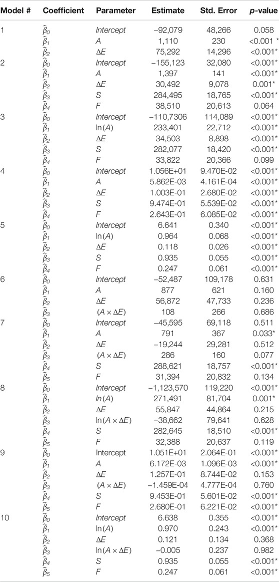
TABLE 4. Parameter estimate, standard error, and p-value for multiple regression models.

The criteria for selecting the best among the ten proposed models are the fulfillment of the statistical regression assumptions, p-value significance for all independent variables, adjusted R², and minimization of 10-fold CV RMSE. According to Table 5 the only models passing the main assumptions of multiple linear regression are the exponential models (i.e., Models 4 and 9 with log transformation of dependent variable C).

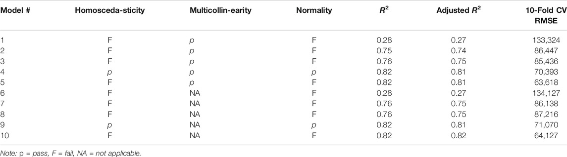
TABLE 5. Model evaluation results for multiple regression models.

Although Model 4 appears to be the preferred model for the first three criteria, Model 5 has a lower 10-fold CV RMSE with equal adjusted R². However, regression assumptions of normality and homoscedasticity of residuals were not satisfied. In the residual plots of normal Q-Q, scale location, and residuals vs. leverage (Figure 2), observations numbered 77, 100, and 101 were detected as problematic observations (2% of total).

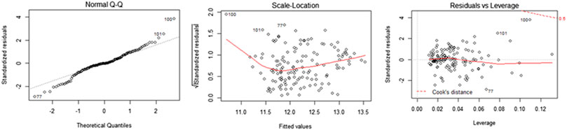
FIGURE 2. Model 5 residuals plots of normal Q-Q, scale location, and residuals vs. leverage.

Examination of the corresponding buildings for these observations revealed that they are extraordinary projects with an unusual A or E (Table 6). For instance, observation #77 has a very low building cost while the building area is large. Therefore, in Model 5m, these three observations were excluded from Model 5, which then satisfied the regression assumptions (Figure 3).

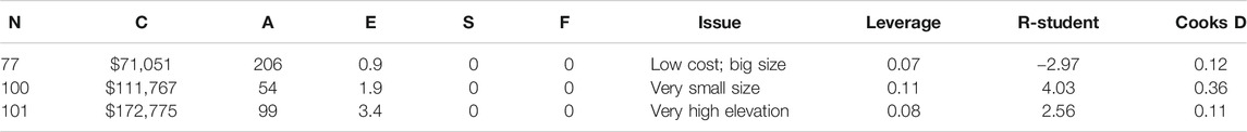
TABLE 6. Outlier observations in model 5 with the description of the issue.

FIGURE 3. Model 5 m residuals plots of normal Q-Q, scale location, and residuals vs. leverage (Model 5 after deleting observations 77, 100, and 101).

Table 7 provides the estimated coefficients, standard errors, and p-values for the Model 5 mm parameters. The p-values are significant for all parameters in the model and the high R² and adjusted R² values of 0.86 and 0.85, respectively, indicate a good fit between data and model. Additionally, the 10-fold CV RMSE is decreased and changed to 61,542. The results for the Model 5 m reveal no violation of tested assumptions (i.e., the p-value of the Shapiro-Wilk test for the normality assumption is 0.063, the p-value of the Breusch-Pagan test for the homoscedasticity assumption is 0.559, and the VIF results for all regressor variables are less than the threshold of 10 [VIF_A = 1.06, VIF_∆E = 1.14, VIF_S = 1.18, VIF_F = 1.04]).

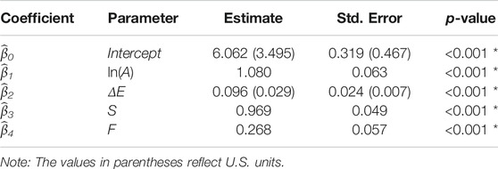
TABLE 7. Parameter estimate, standard error, and p-value for multiple regression model 5 m.

Random Forest and Generalized Additive Model

The random forest model out-of-bag (OOB) error decreased dramatically with the first 50 trees, after which the test-error becomes nearly constant (Figure 4). Therefore, random forest is applied with 800 trees to obtain the best results. The random forest variable importance option indicates that S, A, ∆E, and F are the most important variables in the random forest model, in order.

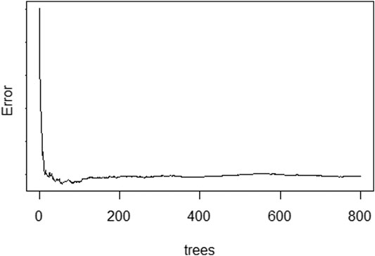
FIGURE 4. Random forest OOB error based on the number of trees.

The 10-fold CV RMSE for the random forest model is 72,843, which is greater than the best regression model. The RMSEs for five GAMs on Models 11–15 are: 89,728, 68,080, 65,182, 64,641, and 64,200, respectively. The results show that Model 15 with logarithmic transformation of response and A variables and spline smoothing on ΔE variable with two degrees of freedom has the best RMSE among all the other GAMs. The partial residual plots of this model show the nonlinear effect of regressors ln(A) and ΔE (Figure 5). We find that ΔE is essentially linear in nature, whereas the ln(A) effect requires mild flexibility.

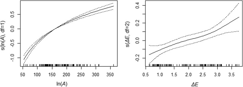
FIGURE 5. Model 15 partial residual plots.

The 10-fold CV RMSEs in the statistical cost estimation models show that the regression Model 5 m (10-fold CV RMSE = 61,542) has the best prediction capability. Therefore, this model is selected to use in this research to compare with the elevation costs on the literature. The cost predictions by this model are shown in Appendix Table A1. Figure 6 shows the predicted project cost calculated using the Model 5 m based on A and ΔE for homes with one-story and slab foundation. The other choices of S and F have exactly the same surface, but shifted vertically. The additive structure, and that perhaps GAMs, although having similar structure (see partial residual plots), are overfitting the smooth relationship and thus mildly suffers with external prediction.Comparison With Cost Literature

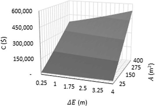
FIGURE 6. Three-dimensional plot of the Model 5 m prediction based on A and ΔE for one-story homes with slab foundations.

In this section, the regression Model 5 m predictions are compared with the USACE (1993), FEMA (1998), and Gair et al (2011) estimates previously described. As a fair basis for comparison, all estimates are adapted to 2015 dollars using Eq. 6 and Louisiana location using Eq. 7. In both Gair et al. (2011) and USACE (1993), the general contractor's charge for overhead and profit is considered to be 10% of the estimated final costs according to the recommendations by these two guidelines. Additionally, Gair et al (2011) estimates include a 5.9% charge for insurance and a 20% contingency factor due to the uncertainty and any unpredicted issue that may happen during the construction work. According to instructions for USACE (1993) estimates, the professional engineering design and landscaping costs must be added to original represented costs in USACE (1993) for elevation.

Table 1 shows the elevation cost based on USACE (1993), FEMA (1998), and Gair et al (2011) cost guidance and regression prediction for one-story buildings in six specific case studies. In all examined case studies, elevation of buildings with existing slab foundations is more expensive than elevation of buildings with other foundation types.

Figure 7 demonstrates graphically the difference between the predicted elevation cost using regression models and cost guidance estimates. The results indicate that USACE (1993) and FEMA (1998) estimates are lower than those in Gair et al. (2011) and regression approaches employed here.

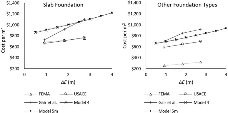
FIGURE 7. Average cost/m² to elevate a one-story home with slab foundation (left) and other foundation types (right).

Discussion

The statistical prediction model is based on the generalization from real and completed elevation projects; therefore, it gives a more realistic estimation with actual cost varieties in the market. Additionally, because a wide range of buildings with different conditions was used in the statistical prediction model, it is able to predict cost based on simple achievable building attributes. The elevation cost comparison in Table 1 and Figure 7 shows that elevating other foundation types is considerably less expensive than elevating slab foundations. Also, for slab foundation elevation, USACE and FEMA guidance underpredict Louisiana elevation costs; for other foundations, FEMA continues to underpredict, but USACE is closer to Louisiana costs.

The partial plot of the selected GAM model shows that cost has a nonlinear relationship with building average floor area. Therefore, the previous cost guidance (USACE, 1993; FEMA, 1998; Gair et al., 2011) that estimates elevation cost only with a single building size, and then generalizes the cost based on that case study, biases results in buildings with different average floor area. Furthermore, the random forest model shows that the number of stories is the most important variable in prediction of elevation project cost, but this variable is not included in current elevation cost guidance.

However, none of the three above-mentioned guidelines have evaluated the effect of important variables such as the building average floor area and number of stories. The USACE (1993) and FEMA (1998) estimates are lower than the newer estimates by Gair et al (2011) and statistical prediction models. The differences may come from changing the construction techniques and equipment over time, and the inherent error in cost adjustment over time. This result suggests that the USACE (1993) and FEMA (1998) guidelines do not have advantages over the newer estimates by Gair et al. (2011) and the statistical prediction models described here. The Gair et al. (2011) study is more conservative than other cost guidance because it considers the 25% contingency factor for any unpredictable construction activities.

Among the tested regression models, Model 5 has the best external prediction ability, with all significant coefficient variables, higher adjusted R², and lower 10-fold CV RMSE. But unlike Model 4, which satisfies all regression assumptions, the normality and homoscedasticity assumptions may be violated based on the p-values of these tests, which fall below the significance level of 0.05. Therefore, this study suggests using the modified Model 5 (i.e., Model 5 m) with trimmed outliers, because it passes all regression assumptions. However, the trimmed otliers did not considerably change the trendline of Model 5 as the plots of Models 5 and 5 m are nearly identical (Figure 6). The random forest and GAM prediction accuracy are inferior to that of regression Models 5 and 5 m. Accordingly, the regression Model 5 m has a better prediction ability for C among all the models and is selected for use in this study. Also, the regression models are preferable to random forest and GAM in ease of interperation and prediction of the results because the equation and estimated coefficents can be used easily to estimate the dependent variable without using sophisticated computer programs.

The cost as calculated in statistical predictions can change based on variables that do not exist in the current guidelines. However, regression Model 5 m shows a substantial agreement between its predictions and the guidelines. For instance, there is a difference of between 0.1 and 24.4% in the Model 5 m estimates vs. Gair et al. (2011) case studies. Therefore, the results suggest that project cost prediction with regression Model 5 m enhances future BCA for flood-mitigated properties.

Conclusion and Summary

To provide a series of building elevation project cost case studies based on cost guidance, this study adjusted the costs in the available guidance to represent those in year 2015 for a Louisiana location. According to the cost guidance results for single-family homes with three levels of elevation and three disparate cost analyzing methods, the occupancy phase elevation cost with USACE estimation is between $590/m² ($55/ft²) and $760/m² ($71/ft²), with FEMA estimation falling between $260/m² ($24/ft²) and $750/m² ($70/ft²), and the Gair et al. (2011) method suggesting between $700/m² ($65/ft²) and $1,100/m² ($99/ft²).

To find an appropriate statistical prediction model, ten regression models along with one random forest model and five GAMs were studied for cost modeling. The correlation matrix prior to regression analysis shows the existence of correlation between cost and all independent variables. However, according to the random forest variable importance function, elevation cost is most strongly affected by the number of stories ─ an attribute that has been neglected in previous elevation cost guidance ─ and change in elevation.

The regression 10-fold CV RMSE results suggest that a log-semi-log model without an interaction term and with trimmed outliers (i.e., Model 5 m) has the lowest RMSE among the tested regression models. In addition, this model makes all independent variables significant with no violation of statistical assumptions and high goodness of fit with R² of 0.85. Therefore, the results suggest that regression models can be used successfully in project cost prediction for elevation projects to address the cost issue in BCA and to overcome barriers in existing cost guidance methods.

The regression study shows that for projects undertaken in Louisiana with adjusted costs to 2015 dollars, the elevation costs for slab foundations are $908/m² ($84/ft²) to elevate 3 ft, $991/m² ($92/ft²) to elevate 6ft, and $1,081/m² ($100/ft²) to elevate 9ft. The elevation costs for other foundation types are $695/m² ($65/ft²) to elevate 3ft, $758/m² ($70/ft²) to elevate 6ft, and $827/m² ($77/ft²) to elevate 9ft.

In recent decades new data collection technologies make data more available for analysis in machine learning prediction models. The results suggest that statistical data prediction models in this study can be used successfully in cost estimation for construction projects, especially for estimation of project costs in natural hazard mitigation projects. However, the statistical modeling of cost in this study suggests that proper model selection is important for improving model prediction. For instance, the RMSE in regression modeling can be improved substantially by choosing proper independent variables and transformation on regression variables specifically when the variables are not distributed normally. The random forest error is decreased by selection of the proper number of trees and the RMSE in GAM analysis can be improved by transformation of variables, applying the smoothing functions on proper variables, and changing the degrees of freedom for smoothing functions.

In future studies, the same methodology can be used for prediction of elevation cost for new buildings during the construction phase. Such information would be useful for adjusting economically the elevation mitigation benefits for new buildings and comparing that estimate with elevation cost in the occupancy phase. Additionally, by knowing the additional cost of elevation in new construction, builders could offer the choice of freeboard (elevation higher than BFE) to the owners as an option for construction in floodprone areas. Also in future studies, the mitigation cost can be predicted by statistical methods for other types of mitigation projects, such as hurricane and tornado wind mitigations.

Data Availability Statement

The data that support the findings of this study are available from the Louisiana Governor’s Office of Homeland Security and Emergency Preparedness. Restrictions apply to the availability of these data, which were used under license for this study.

Author Contributions

AT and CF contributed conception and design of the study; JG provided data; AT and CF organized the database; AT performed the statistical analysis; BM helped with statistical analysis; IN provided instructions to improve the paper quality; AT wrote the first draft of the manuscript; and RR wrote sections of the manuscript. All authors contributed to manuscript revision, read and approved the submitted version.

Funding

This research was supported by FEMA Grant 4080-DR-LA (Project 0017 Statewide Hazard Mitigation Community Education and Outreach Project, CFDA 97–039) through the GOHSEP “Economic Benefit of Mitigation” Project.

Conflict of Interest

The authors declare that the research was conducted in the absence of any commercial or financial relationships that could be construed as a potential conflict of interest.

Acknowledgments

Any opinions, findings, conclusions, or recommendations expressed in this paper are those of the authors and do not necessarily reflect the views of FEMA or GOHSEP. This paper is part of a dissertation submitted to the graduate school at Louisiana State University (LSU) and appeared online through the university’s digital commons. Also, the publication of this article is subsidized by the LSU Libraries Open Access Author Fund.

References

Appendix A. Elevation project cost estimates

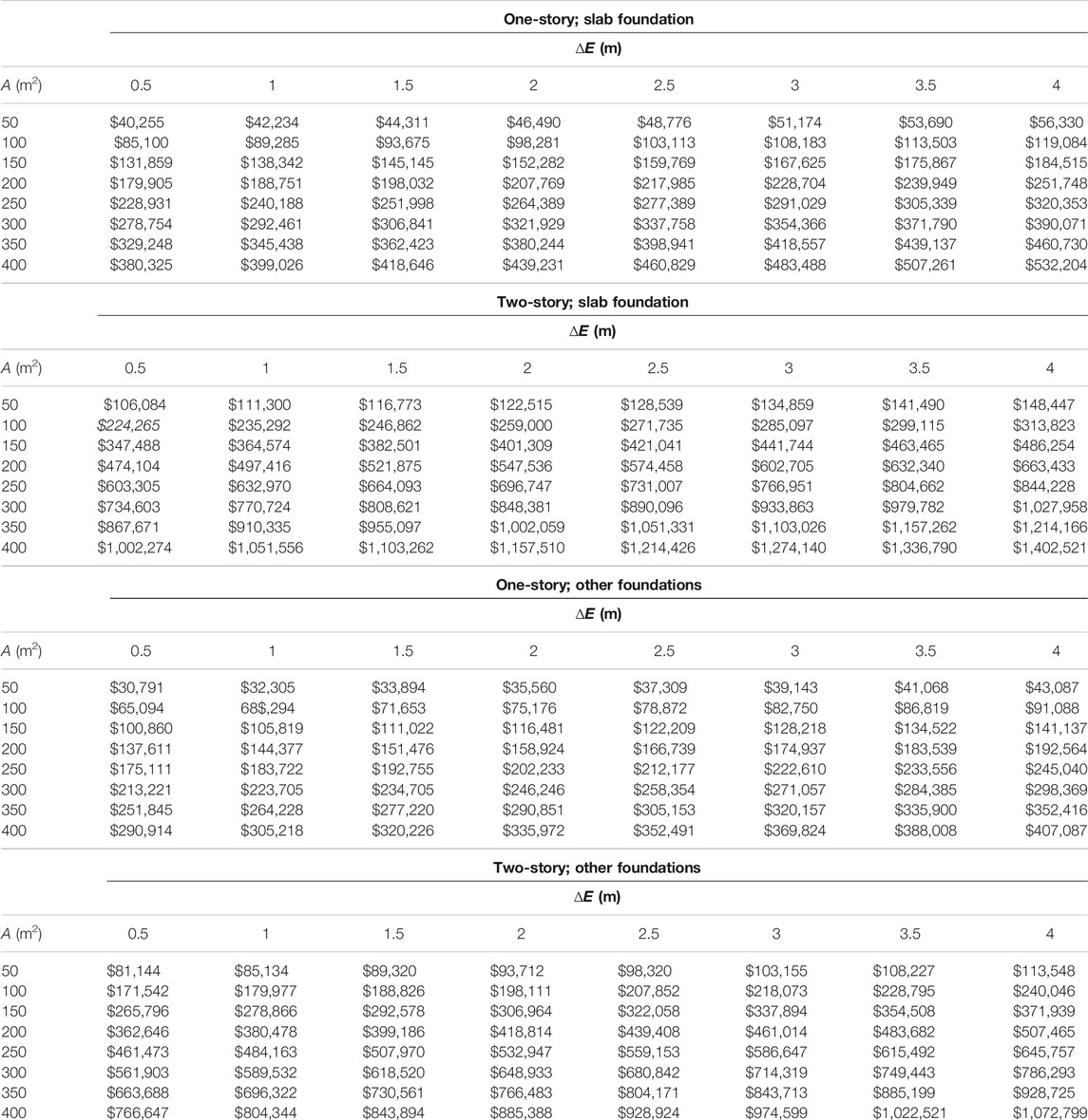
TABLE A1. Elevation project cost estimates by the selected regression model (Model 5 m).

References

Adeli, H., and Wu, M. (1998). Regularization Neural Network for Construction Cost Estimation. J. Construction Eng. Manag. 124 (1), 18–24. doi:10.1061/(asce)0733-9364(1998)124:1(18)
Amoroso, S. D., and Fennell, J. P. (2008). A Rational Benefit/cost Approach to Evaluating Structural Mitigation for Wind Damage: Learning "the Hard Way" and Looking Forward. Proc. Structures Congress, 1–10. doi:10.1061/41016(314)249
Andersen, R. (2008). Modern Methods for Robust Regression. Newbury Park, CA, United States: Sage. doi:10.4135/9781412985109
Atici, U. (2011). Prediction of the Strength of mineral Admixture concrete Using Multivariable Regression Analysis and an Artificial Neural Network. Expert Syst. Appl. 38 (8), 9609–9618. doi:10.1016/j.eswa.2011.01.156
Bellomo, D., Pajak, M. J., and Sparks, J. (1999). Coastal Flood Hazards and the National Flood Insurance Program. J. Coastal Res., 21–26.
Bohn, F. (2013). “Design Flood Elevations beyond Code Requirements and Current Best Practices,”. Master’s thesis(Baton Rouge, LA: Louisiana State University).
Breusch, T. S., and Pagan, A. R. (1979). A Simple Test for Heteroscedasticity and Random Coefficient Variation. Econometrica 47, 1287–1294. doi:10.2307/1911963
Calabrese, R., and Osmetti, S. A. (2015). Improving Forecast of Binary Rare Events Data: A GAM-Based Approach. J. Forecast. 34 (3), 230–239. doi:10.1002/for.2335
Cutler, D. R., Edwards, T. C., Beard, K. H., Cutler, A., Hess, K. T., Gibson, J., et al. (2007). Random Forests for Classification in Ecology. Ecology 88 (11), 2783–2792. doi:10.1890/07-0539.1
FEMA, (2012). “Engineering Principles and Practices of Retrofitting Floodprone Residential Structures,” in Department of Homeland Security (Washington, DC: Federal Emergency Management Agency).
FEMA, (2010). “Home Builder’s Guide to Coastal Construction,” in Department of Homeland Security (Washington, D.C: Federal Emergency Management Agency).
FEMA, (1998). “Homeowner's Guide to Retrofitting; Six Ways to Protect Your House from Flooding,” in Department of Homeland Security (Washington, D.C: Federal Emergency Management Agency).
FEMA, (2011). “Supplement to the Benefit-Cost Analysis Reference Guide,” in Department of Homeland Security (Washington, DC: Federal Emergency Management Agency).
Gair, R., Balboni, B., Phelan, M., Charest, A., Waier, P., and Mossman, M. J. (2011). Final Report–Louisiana House Raising–Slab on Grade and Pier and Beam Construction. RS Means: Reed Construction Data.
Grogan, T. (2016). How to Use ENR’s Indexes. Available at: http://enr.construction.com/economics/historical_indices/(Accessed August 10, 2017). doi:10.4324/9781315255712
Han, S.-R., Guikema, S. D., and Quiring, S. M. (2009). Improving the Predictive Accuracy of Hurricane Power Outage Forecasts Using Generalized Additive Models. Risk Anal. 29 (10), 1443–1453. doi:10.1111/j.1539-6924.2009.01280.x
Hastie, T. (2020). Generalized Additive Models: Package ‘gam’. Available at: https://cran.r-project.org/web/packages/gam/gam.pdf (Accessed December 1, 2020).
Herbsman, Z. (1986). Model for Forecasting Highway Construction Cost. Gainesville, FL, United States: Transportation Research Record (1056).
Jafarzadeh, R., Ingham, J., Walsh, K., Hassani, N., and Ghodrati Amiri, G. (2015). Using Statistical Regression Analysis to Establish Construction Cost Models for Seismic Retrofit of Confined Masonry Buildings. J. Construction Eng. Manag. 141 (5), 04014098. doi:10.1061/(asce)co.1943-7862.0000968
Jrade, A., and Alkass, S. (2007). Computer-integrated System for Estimating the Costs of Building Projects. J. Archit. Eng. 13 (4), 205–223. doi:10.1061/(asce)1076-0431(2007)13:4(205)
Karshenas, S. (1984). Predesign Cost Estimating Method for Multistory Buildings. J. Construction Eng. Manag. 110 (1), 79–86. doi:10.1061/(asce)0733-9364(1984)110:1(79)
Kim, G.-H., An, S.-H., and Kang, K.-I. (2004). Comparison of Construction Cost Estimating Models Based on Regression Analysis, Neural Networks, and Case-Based Reasoning. Building Environ. 39 (10), 1235–1242. doi:10.1016/j.buildenv.2004.02.013
Kohavi, R. (1995). A Study of Cross-Validation and Bootstrap for Accuracy Estimation and Model Selection. Proceedings of the 14th international joint conference on Artificial intelligence, Montreal, Quebec, Canada Vol. 2, 1137–1145.
Kouskoulas, V., and Koehn, E. (1974). Predesign Cost Estimating Function for Buildings. J. Construct. Div. 100 (4), 589–604. doi:10.1061/JCCEAZ.0000461
Larsen, K. (2015). “GAM: The Predictive Modeling Silver Bullet,” in Multithreaded (San Francisco, CA, United States: Stitch Fix), 30.
Li, Y., and van De Lindt, J. W. (2012). Loss-based Formulation for Multiple Hazards with Application to Residential Buildings. Eng. Structures 38, 123–133. doi:10.1016/j.engstruct.2012.01.006
Liu, X., Song, Y., Yi, W., Wang, X., and Zhu, J. (2018). Comparing the Random Forest with the Generalized Additive Model to Evaluate the Impacts of Outdoor Ambient Environmental Factors on Scaffolding Construction Productivity. J. Construction Eng. Manag. 144 (6), 04018037. doi:10.1061/(asce)co.1943-7862.0001495
Lowe, D. J., Emsley, M. W., and Harding, A. (2006). Predicting Construction Cost Using Multiple Regression Techniques. J. Constr. Eng. Manage. 132 (7), 750–758. doi:10.1061/(asce)0733-9364(2006)132:7(750)
Lumley, T., Diehr, P., Emerson, S., and Chen, L. (2002). The Importance of the Normality assumption in Large Public Health Data Sets. Annu. Rev. Public Health 23 (1), 151–169. doi:10.1146/annurev.publhealth.23.100901.140546
Mikhed, V., and Zemčík, P. (2009). Do house Prices Reflect Fundamentals? Aggregate and Panel Data Evidence. J. Housing Econ. 18 (2), 140–149. doi:10.1016/j.jhe.2009.03.001
Montgomery, D. C., Peck, E. A., and Vining, G. G. (2015). Introduction to Linear Regression Analysis. United States: John Wiley & Sons.
Moore, L., Hanley, J., Turgeon, A., and Lavoie, A. (2011). A Comparison of Generalized Additive Models to Other Common Modeling Strategies for Continuous Covariates: Implication for Risk Adjustment. J. Biomet Biostat 2 (1), 109. doi:10.4172/2155-6180.1000109
Orooji, F., and Friedland, C. J. (2017). Cost-benefit Framework to Generate Wind hazard Mitigation Recommendations for Homeowners. J. Architectural Eng. 23 (4), 04017019. doi:10.1061/(asce)ae.1943-5568.0000269
Popescu, C. M., Phaobunjong, K., and Ovararin, N. (2003). Estimating Building Costs. Oxfordshire, United Kingdom: CRC Press.
Priddy, K. L., and Keller, P. E. (2005). Artificial Neural Networks: An Introduction. Bellingham, Washington, United States: SPIE Press. doi:10.1117/3.633187
Renn, O. (1998). Three Decades of Risk Research: Accomplishments and New Challenges. J. Risk Res. 1 (1), 49–71. doi:10.1080/136698798377321
RSMeans, (2015). Building Construction Cost Data (73rd annual edition ed.), Gordian Group, Rockland, MA, United States: The Gordian Group, Inc.
Shapiro, S. S., and Wilk, M. B. (1965). An Analysis of Variance Test for Normality (Complete Samples). Biometrika 52 (3/4), 591–611. doi:10.1093/biomet/52.3-4.591
Shimizu, C., Karato, K., and Nishimura, K. (2014). Nonlinearity of Housing price Structure. Int. J. Housing Markets Anal. 7 (4), 459–488. doi:10.1108/ijhma-10-2013-0055
Skitmore, R. M., and Ng, S. T. (2003). Forecast Models for Actual Construction Time and Cost. Building Environ. 38 (8), 1075–1083. doi:10.1016/S0360-1323(03)00067-2
Sonmez, R. (2008). Parametric Range Estimating of Building Costs Using Regression Models and Bootstrap. J. Constr. Eng. Manage. 134 (12), 1011–1016. doi:10.1061/(asce)0733-9364(2008)134:12(1011)
Sousa, S., Martins, F., Alvimferraz, M., and Pereira, M. (2007). Multiple Linear Regression and Artificial Neural Networks Based on Principal Components to Predict Ozone Concentrations. Environ. Model. Softw. 22 (1), 97–103. doi:10.1016/j.envsoft.2005.12.002
Taghinezhad, A., Friedland, C. J., and Rohli, R. V. (2020a). Benefit-cost Analysis of Flood-Mitigated Residential Buildings in Louisiana. Oxfordshire, United Kingdom: Taylor & Francis, 1–18.
Taghinezhad, A., Friedland, C. J., Rohli, R. V., and Marx, B. D. (2020b). An Imputation of First-Floor Elevation Data for the Avoided Loss Analysis of Flood-Mitigated Single-Family Homes in Louisiana, United States. Front. Built Environ. 6 (138). doi:10.3389/fbuil.2020.00138
Touran, A., and Lopez, R. (2006). Modeling Cost Escalation in Large Infrastructure Projects. J. Constr. Eng. Manage. 132 (8), 853–860. doi:10.1061/(asce)0733-9364(2006)132:8(853)
USACE (1993). Flood Proofing: How to Evaluate Your Options. Washington DC, United States: US Army Corps of Engineers.
Waier, P. R., and Balboni, B. (2018). Building Construction Cost Data. Rockland, MA, United States: RS Means Company.
Wilmot, C. G., and Mei, B. (2005). Neural Network Modeling of Highway Construction Costs. J. Constr. Eng. Manage. 131 (7), 765–771. doi:10.1061/(asce)0733-9364(2005)131:7(765)
Xiang, D. (2001). Fitting Generalized Additive Models with the GAM Procedure. Proc. SUGI Proceedings, Citeseer, 256–226.
Zhang, F., Lai, T., Rajaratnam, B., and Zhang, N. R. (2011). Cross-Validation and Regression Analysis in High-Dimensional Sparse Linear Models. Stanford, CA, United States: Stanford University. doi:10.1109/icip.2011.6116121