On the mathematical modeling of schistosomiasis transmission dynamics with heterogeneous intermediate host
 Chinwendu E. Madubueze
 Z. Chazuka
 I. O. Onwubuya
 F. Fatmawati3
  C. W. Chukwu
- 1Department of Mathematics, Joseph Sarwuan Tarka University, Makurdi, Nigeria
- 2Department of Decision Sciences, College of Economic and Management Sciences, University of South Africa, Pretoria, South Africa
- 3Department of Mathematics, Faculty of Science and Technology, Universitas Airlangga, Surabaya, Indonesia
- 4Department of Mathematics, Wake Forest University, Winston-Salem, NC, United States
Schistosomiasis is a neglected disease affecting almost every region of the world, with its endemicity mainly experience in sub-Saharan Africa. It remains difficult to eradicate due to heterogeneity associated with its transmission mode. A mathematical model of Schistosomiasis integrating heterogeneous host transmission pathways is thus formulated and analyzed to investigate the impact of the disease in the human population. Mathematical analyses are presented, including establishing the existence and uniqueness of solutions, computation of the model equilibria, and the basic reproduction number (R0). Stability analyses of the model equilibrium states show that disease-free and endemic equilibrium points are locally and globally asymptotically stable whenever R0 < 1 and R0>1, respectively. Additionally, bifurcation analysis is carried out to establish the existence of a forward bifurcation around R0 = 1. Using Latin-hypercube sampling, global sensitivity analysis was performed to examine and investigate the most significant model parameters in R0 which drives the infection. The sensitivity analysis result indicates that the snail's natural death rate, cercariae, and miracidia decay rates are the most influential parameters. Furthermore, numerical simulations of the model were done to show time series plots, phase portraits, and 3-D representations of the model and also to visualize the impact of the most sensitive parameters on the disease dynamics. Our numerical findings suggest that reducing the snail population will directly reduce Schistosomiasis transmission within the human population and thus lead to its eradication.
1. Introduction
Schistosomiasis which is also known as Bilharzia, Bilharziasis, and snail fever, is one of the neglected tropical diseases (NTD) common in some tropical and subtropical countries, in areas where there is no access to safe drinking water, adequate hygiene, and appropriate sanitation (sewage disposal). It is a water-based disease that is transmitted through contact with water infested with cercariae and it affects about 240 million people worldwide and more than 700 million people live in an area where the disease is endemic [1]. Schistosomiasis infection is also known as a parasite disease that is caused by schistosomiasis organisms (blood fluke). The two main forms of schistosomiasis infection are urogenital and intestinal which are caused by five schistosomiasis species responsible for human or animal infections namely, Schistosoma mansoni, Schistosoma intercalatum, Schistosoma haematobium, Schistosoma mekonai, and Schistosoma japonicum [1]. There are two stages of schistosomiasis infection namely; acute and chronic stages. Acute schistosomiasis infection referred to as Katayama Syndrome is a clinical manifestation of infection caused by trematode worms [2].
When non-immune persons are exposed to schistosomiasis infection, there is an incubation period symptoms of infection include abdominal pain, blood in stool or urine, wasting, anemia, dysuria [2]. Chronic schistosomiasis infection is caused by schistosome, which has severe long-term implications [3]. The symptoms of the chronic stage are growth retardation, renal failure, ascites, grand mal epilepsy, decreased fitness, anemia, portal hypertension, transverse myelitis, bladder carcinoma, and infertility [2]. Normally, snails harbor cercariae and shed the infective stage (cercariae) of the parasite (schistosome) in the freshwater [4]. Hence, there is an increase in the prevalence of Schistosomiasis as a result of freshwater habitats such as dams and irrigation, which enhances snail habitation and thus, increases transmission. Despite the progressive achievements in schistosomiasis control over the years, Schistosomiasis is still one of the most devastating parasitic diseases ravaging the entire world. Guiro et al. [5] proposed a mathematical model for schistosomiasis control, considering two population hosts, humans, and snails with delays. Their results suggest that an effective education campaign and reasonable coverage level of drug treatment will help in the control of Schistosomiasis. A mathematical model for the human-cattle-snail transmission of Schistosomiasis in Hubei Province, China was studied by Chen et al. [6]. Their results show that to control or eliminate Schistosomiasis in Hubei Province, China. Environmental factors need to be considered to lower (narrow) cattle-snail transmission. Since chemotherapy alone cannot end the spread of the causative parasite (schistosome), additional interventions and control strategies must be combined to lower re-infection, reduce the prevalence, and move toward the elimination of Schistosomiasis [7]. Many researchers have considered the use of molluscicides and different kinds of environmental modifications to control snails to reduce or eliminate schistosomiasis prevalence [7–9]. Interested readers can also see the following references [10–20] for other published works that have used mathematical models to gain insight into the transmission dynamics of Schistosomiasis and other infectious diseases in the human population and various suggestion for their control/elimination.
Given the aforementioned above, our study presents a mathematical modeling work that examines qualitative mathematical analysis for the prevention and control of the spread of Schistosomiasis through the control of snails. This is in addition to chemotherapy, molluscicides, and other environmental factors already studied in the previous research works and also the inclusion of the acute and chronic infected populations (compartments). The present study also investigates if mammals such as cattle contribute to the spread of Schistosomiasis infection within the population. The model described in this work considers three population hosts that is: humans, cattle, and snails.
The paper is organized as follows: Section 2 gives the Model formulation, Section 3 the Mathematical model analysis is presented, Section 4 presents the Sensitivity analysis of parameters in the model, Section 5 presents the Results of the numerical simulations and finally, Section 6 gives a brief Discussion and Conclusion.
2. Model formulation
The life cycle of the schistosome parasite is formulated mathematically. The populations considered are the human population, other mammal population, and snail population with the Cercariae C(t) and Miracida M(t). Cercariae C(t) is a larva worm that the infected snails shed into the aquatic environment, while the Miracida M(t) are eggs that the infected mammals (human and other mammals) shed in the stream when they come to the river for human activities such as fishing, swimming, fetching water, and/or drinking of water by other mammals. In this study, other mammals include cattle, mice, and dogs that the schistosome parasite can infect. The total human population, Nh(t), at time, t, is divided into the sub-populations; susceptible, Sh(t), acute infected, IA(t), and chronic infected, Ich(t) humans. The other mammal population, Na(t), is subdivided into susceptible mammals, Sa and infected mammals, Ia, while the snail population, Ns(t) is made up of susceptible snails, Ss(t) and infected snails Is(t). Human recruitment and natural death rates are assumed to be Λh and μh, respectively. The susceptible humans, Sh(t), become infected through contact with fresh water contaminated with Cercariae from infected snails. The force of infection is given by
where βh is the human transmission rate, αh is the adult parasite production rate for humans, C0, is the half-saturation constant of Cercariae within the environment and ε1 is the limitation of the growth velocity of the pathogens for Cercariae. Susceptible humans become acutely infected upon infection and enter into class, IA(t). In the acutely infected sub-population, a proportion of them may recover with partial immunity depending on the mass drug administration program within the community and return to the susceptible class at a rate, ψ. On the other hand, some human may develop a chronic infection at a rate, k and move to class, Ich. Chronically infected humans may succumb to infection at a rate, δh. Shedding of infection within the environment by acute infected and chronic infected humans is assumed to occur at rate NEτ1γh and NEτ1γhσ, respectively. Here, NE is the number of eggs shed by mammals (both human and other mammals), τ1 is the probability of eggs developing into Miracidium, γh is the infected human shedding rate and σ is a parameter that influences the shedding rate of the chronically infected humans. For the other mammals, the recruitment rate is assumed to be Λa while the natural death rate is μa. The susceptible mammals are infected through contact with fresh water contaminated with Cercariae from infected snails and the force of infection is given by
where βa is the other mammal transmission rate, αa, is the adult parasite production probability for other mammals. The other mammals shed the eggs that hatch into the water at a rate, NEτ1γa where γa is the other mammals shedding rate. Death due to infection among other infected mammals is assumed to be at a rate, δa. Furthermore, susceptible snails are recruited at a rate, Λs and death due to natural causes of snails is at a rate, μs. Susceptible snails become infected by contact with miracidia from the viral shedding of infected humans and other mammals and the force of infection is given by
where βs, is the snail transmission rate, αs is the Miracidial penetration probability for snails, ε2, is the limitation of the growth velocity for the Miracidium and M0, is the half-saturation constant for Miracida within the environment. Death due to infection of snails is assumed to be at a rate, δs. Infected snails shed larva worm in the environment at a rate, τ2γs where τ2 is the density of Cercariae for snails and γs is the snail shedding rate. Finally, the decay rates for the Cercariae and Miracida are μc, μM, respectively. The study assumes that there is no immigration of infectious humans, other mammals, and snails within their populations. Also, susceptible humans, other mammals and snails are recruited at a constant rate. The dynamics of infection are presented in the model flow diagram in Figure 1. This leads to the following system of non-linear differential equations:
with initial conditions
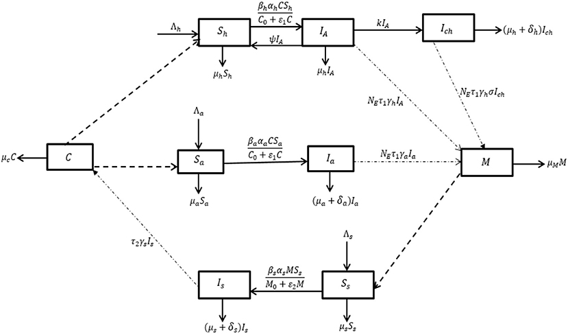
Figure 1. Flow diagram for the dynamics of Schistosomiasis infection.
All the parameters are assumed to be non-negative over the modeling time frame.
3. Mathematical methods
3.1. Invariant region
A biologically feasible population model such as model system (4) should always have positive solutions. To show that all solutions of model system (4) are non-negative, we let Nh, Na and Ns be the total human population, other mammals population and snail populations, respectively, where, Nh(t) = Sh(t) + IA(t) + Ich(t), Na(t) = Sa(t) + Ia(t), and Ns(t) = Ss(t) + Is(t), respectively with the initial conditions Nh(0), Na(0), Ns(0), M(0), and C(0).
Adding the human, other mammals and snail populations give the respective total populations as and . In the absence of infection which implies that the disease-related death rates for chronically infected human, δh, other infected mammals, δa and infected snail, δs are negligible, we assume that the total populations, Nh, Na and Ns are asymptotically stable and yield
Solving (5) using the inequality theorem by Birkhoff and Rota [21] and integrating with the initial conditions Nh(0), Na(0), Ns(0), C(0), and M(0) gives
As t → ∞, the total populations for humans, other mammals and snails approach , and , respectively. Since IA, Ich ≤ Nh(t), Ia ≤ Na(t), and Is ≤ Ns(t) it implies that the Cercariae (C) and Miracidia (M) populations can be written as
Applying the inequality theorem by Birkhoff and Rota [21] with the initial conditions C(0) = C00 and M(0) = M00 yields
and
As t → ∞, the Cercariae and Miracidia populations tends to respectively.
This shows that all the feasible solutions Nh(t), Na(t), Ns(t), C(t) and M(t) are bounded and the region,
is positively invariant. Thus, we conclude that for all t>0, model system (4) is biologically feasible and well-posed in .
3.2. Positivity of the solution
We show that the solutions of the model system (4) are positive for all time by proving the following theorem:
Theorem 3.1. With positive initial conditions, the solution set of model system (4), [Sh(t),IA(t),Ich(t), Sa(t), Ia(t), M(t), Ss(t), Is(t), C(t)], is positive for all time, t > 0.
Proof. From the first equation of the model Equation (4), we have
Integrating with initial condition Sh(0), we obtain
with
In a similar way with and
Therefore, we conclude that the solution set [Sh(t), IA(t), Ich(t), Sa(t), Ia(t), M(t), Ss(t), Is(t), C(t)] of model Equation (4) is positive for all t > 0. This shows that the model is well-posed and biologically meaningful since the sub-population cannot be negative.
3.3. Existence of disease-free equilibrium
We examine the stability of the disease-free equilibrium state of the schistosomiasis model system (4) in terms of basic reproduction number. The disease-free equilibrium, E0, is the equilibrium state in the absence of schistosomiasis disease in the environment. At equilibrium state,
This is solved simultaneously for the schistosomiasis model Equation (4) to yield the disease-free equilibrium,
3.3.1. The basic reproduction number
The basic reproduction number of the schistosomiasis model system (4) denoted by R0, is a threshold parameter that is interpreted biologically as the average number of infected individuals created by one infected individual introduced in a susceptible population during the course of its infectious period [22, 23]. We compute R0 using the next-generation matrix approach by Van den Driessche and Watmough [22]. Applying the approach, let and denote the Jacobian matrices for the rates of appearance of new infections and the transfer of infections in and out of the infected compartments, respectively at DFE, E0, so that
where
The basic reproduction number, R0, for the model system (4) is defined as the spectral radius of the operator, , where is the inverse matrix of . This gives
for
Here, the reproduction numbers, RA, Rch, Rm, and Rs, are the reproduction numbers for the acutely infected humans, chronic infected humans, other infected mammals and infected snails contribute, respectively. This shows that the basic reproduction number, R0 of the schistosomiasis model system (4) comprises of four parts, that is, RA, Rch, Rm, Rs. Importantly, whenever R0 < 1, it implies that the disease will fizzle out in the population and whenever R0>1, it means that the disease will persist in the population.
3.4. Local stability of the disease-free equilibrium
We prove the local stability of the disease-free equilibrium, E0, for the Schistosomiasis model system (4) using the Jacobian method.
Theorem 3.2. The disease-free equilibrium state, E0, of the schistosomiasis model system (4) is locally asymptotically stable when R0 < 1 and unstable for R0 > 1.
Proof. We compute the Jacobian matrix of the model system (4) at the equilibrium state, E0, as follows.
where f, g, h, q, A, B, D are defined in (12). The eigenvalues of (15) are λ1 = −μh, λ2 = −μa, λ3 = −μs and the roots of the characteristics equation
where
With the definitions of reproduction numbers in (14), we have by Routh-Hurwitz criteria in Kim et al. [24] and the conditions in Heffernan et al. [25] that the polynomial in (16) has negative real roots provided that P > 0, Q > 0, R > 0, U > 0, V > 0, W > 0, PQ > R, QU > W, UV > RW and this happens when R0 < 1. With negative real eigenvalues, it implies that the disease-free equilibrium state, E0, for Schistosomiasis model system (4) is locally asymptotically stable if R0 < 1 otherwise it is unstable.
3.5. Existence of endemic equilibrium
For the endemic equilibrium, let
in model system (4). We have at equilibrium state that
Substituting , and C* into and and solve simultaneously, we obtain
with as solution of the polynomial
where
Solving (20) for , it can be seen that one of the solutions is which represents the disease-free equilibrium state, while the other solution of the polynomial (20) is the endemic equilibrium state of the model system (4) that is given by
and it is positive whenever R0 > 1. We further use Descarte's rule of signs to discuss the existence of possible positive roots of Equation (18) especially when R0 < 1. The results are summarized in Table 1. Hence, the following theorem.
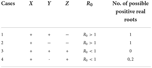
Table 1. No. of possible positive real roots for (20).
Theorem 3.3. System (4) has the following endemic equilibrium:
• If R0 > 1, then the system has one positive unique endemic equilibrium state.
• If R0 < 1, then the system has zero or two endemic equilibria.
In case (4), there is possibility of backward bifurcation of the model system (4) as it may contain endemic equilibrium with DFE when R0 < 1. This is further determine by carrying out a bifurcation analysis in the following subsection.
3.6. Bifurcation analysis
The stability of endemic equilibrium state is established using Center Manifold Theory by Chavez et al. [26]. The theory shows the direction of bifurcation, whether it is a forward or backward bifurcation. A forward bifurcation indicates that the disease-free and endemic equilibrium states are locally asymptotically stable if R0 < 1 and R0 > 1, respectively, which implies the existence of global stability of the equilibrium states. A backward bifurcation means there is a co-existence of disease-free and endemic equilibrium when R0 < 1. Therefore, we apply the theory in Chavez et al. [26] by re-writing the state variables as follows
such that the model system (4) can be rewritten as
where is the right hand side of model system (4).
Let the bifurcation parameter be at R0 = 1 so that the Jacobian matrix, J(E0), of (15) will have a simple zero eigenvalue and negative real eigenvalues. The left and right eigenvectors associated with a simple zero eigenvalue of the Jacobian matrix (15) are w = (w1, w2, w3, w4, w5, w6, w7, w8, w9) and v = (v1, v2, v3, v4, v5, v6, v7, v8, v9), respectively, where
We state and prove the following theorem
Theorem 3.4. Model system (4) undergoes a forward bifurcation at R0 = 1.
Proof. To determine the direction of the bifurcation, Theorem 4.1 in Castillo-Chavez and Song [27] is used to compute the bifurcation coefficients, m and n, of model system (4). The non-zero associated partial derivatives of F at the disease-free equilibrium, E0, are
Now applying the concept of Castillo-Chavez and Song [27], the value of m gives
Upon substituting the eigenvectors and partial derivatives, we obtain
where
Also for n, we have
A forward bifurcation exists since m < 0 in (24) and n > 0 in (26). Therefore, a forward bifurcation exists for the model (4) at R0 = 1. This completes the proof.
With the existence of forward bifurcation, a unique endemic equilibrium, E1, exists and is locally asymptotically stable whenever R0 > 1 and unstable when R0 < 1. Hence, there is possibility of global stability of the equilibrium states. A forward bifurcation plot is shown in Figure 2.
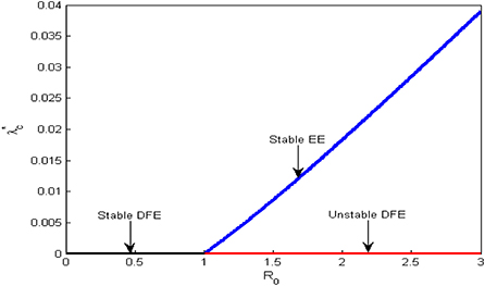
Figure 2. Bifurcation plot for the dynamics of Schistosomiasis.
3.7. Global stability of the model
In this subsection, the global behavior of the disease-free and endemic equilibria of the system (4) is established by constructing a suitable Lyapunov functions and applying LaSalle's invariance principle.
3.7.1. Global stability of disease-free equilibrium, E0
Theorem 3.5. The disease-free equilibrium, E0, of the schistosomiasis model system (4) is globally asymptotically stable when R0 < 1 otherwise unstable.
Proof. Constructing a Lyapunov function using a matrix-theoretic method by [28] gives
where the letters, A, B, and D are defined in (12).
Taking the derivative of Equation (27) along the trajectory yields
Expanding Equation (28) and simplifying in terms of reproduction numbers (RA, Rch, Rm, Rs) gives
With , , , we have
Since RA+Rch+Rm ≤ 1, Rs ≤ 1 from the definition of the reproduction number in (13) and (14), this yields L′ ≤ 0 if R0 < 1. Hence by LaSalle's invariance principle, the disease-free equilibrium is globally asymptotically stable if R0 ≤ 1. This completes the proof.
3.7.2. Global stability of endemic equilibrium, E1
To prove the stability of the endemic equilibrium (E1) we state and prove the following theorem
Theorem 3.6. The endemic equilibrium, E1, of the schistosomiasis model system (4) is globally asymptotically stable whenever R0 > 1 and ψ = 0.
Proof. The global stability of the endemic equilibrium is proved by constructing the Volterra-Lyapunov function
where , , A, B, and D are defined in (12) and (18).
Taking the time derivative of along the solutions of the schistosomiasis model Equation (4) yields
At endemic equilibrium state, we have
Substituting Equation (32) into (31) and expanding and simplifying gives
Using the assumption that ψ = 0 and , , we have by Arithmetic-Geometric Theorem that
This implies that L′ ≤ 0 in the region, Z. Applying LaSalle's invariance principle, the endemic equilibrium state of the schistosomiasis model system (4) is globally asymptotically stable in Z if R0 > 1 and ψ = 0. This means that with different initial conditions at ψ = 0, the global stability of the schistosomiasis model system (4) will always converge to the disease-free and endemic equilibrium states whenever R0 < 1 and R0 > 1, respectively. The numerical simulations are carried out in the next section.
4. Sensitivity analysis
4.1. Parameter values
To perform numerical simulations, parameters for the model are mainly sourced from literature, as shown in Table 2. Parameters that are represented by probabilities are assumed to be within the range of [0 − 1]. Any parameters that are outside the prescribed range are properly sampled from a uniform distribution within ranges defined in Table 2.
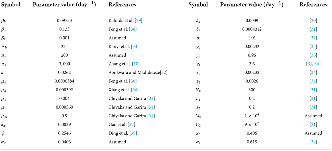
Table 2. Parameter values used for the numerical simulation of model system (4).
4.2. Sensitivity analysis results
Sensitivity analysis examines the relative change of the mathematical model output (variable) when the model parameter(s) are altered or changed. It helps in determining and identifying the model parameters that require special attention. To carry out the sensitivity analysis of the basic reproduction number R0, we adopt the Latin Hypercube Sampling (LHS) scheme and Partial Rank Correlation Coefficients (PRCCs) technique used by Blower and Dowlatabadi [39] to compute and identify the biological implication of each model parameter on R0. See also the following published articles [40–45] with similar analyses for different epidemic models where the LHS techniques have been applied. We performed 1,000 simulations per run and examined and evaluated the PRCC of the model parameters concerning R0. The PRCC values indicate the degree of monotonicity between the parameters of the model and R0. Thus, juxtaposing the PRCC values gives us a clear picture on the contribution of each parameter of the model on R0. Table 3 and the Tornado plot of Figure 3 give the model parameters with their PRCCs. The parameters with the potential of increasing(decreasing) the value of R0, are those with positive(negative) PRCCs. Thereby, increasing parameters, βs, βh, βa, γh, γa, γs, τ1, τ2, increases the value of R0 which in turn increase the spread of schistosomiasis disease within the population (see Table 2 and Figure 3). On the other hand, parameters μc, μm, μs with negative PRCCs influence the reduction of the burden of schistosomiasis disease within the population. When these parameters are increased, we observe a reduction in the value of R0, hence the endemicity of the Schistosomiasis within the population is also reduced. The natural death rate for the snail population is the most sensitive parameter with respect to R0 with a PRCC value of 0.776046728. The implication of this is that increasing snail death rate reduces the spread of Schistosomiasis within the population. To examine the significance of the model parameters, we compute the p-value of PRCC of each model parameter using the Fisher Transformation method as shown in Table 3. Table 3 reveals that the parameters, βs, βh, γh, γs, μc, μm, μs, τ1, τ2 have significant p-values while the parameters, βa, γa, have insignificant p-values. This implies that the shedding and transmission rates of the other mammals, γa and βa, are non-monotonically related to R0, though they can still produce changes in the transmission dynamics of schistosomiasis infection.
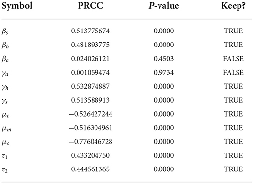
Table 3. PRCC values and significance.
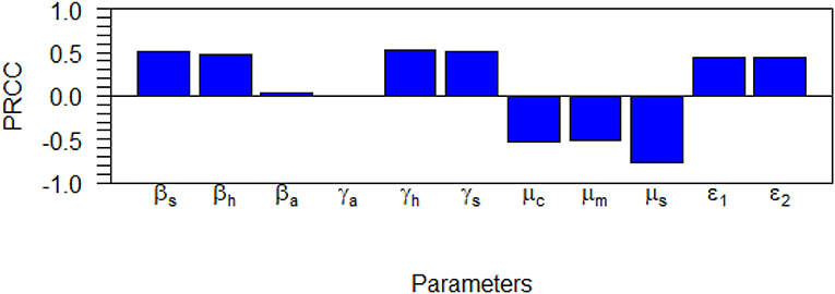
Figure 3. Tornado plot for the dynamics of Schistosomiasis infection on the R0 showing the model parameters with their PRCC values.
The pairwise comparison of the significant parameters of Table 3, whose p < 0.05 is given in Tables 5, 6. The pairwise comparison is carried out to observe the model parameters with notable influence on increasing the burden of the schistosomiasis infection in the population, as well as to establish whether there exists any difference between the processes describing the compared parameters. We presented the outcome of the pairwise PRCC comparison between the unadjusted p-values (Table 4) and the false discovery rate (FDR) adjusted p-values in Tables 5, 6. According to Table 6, whenever the p-values of the compared pair of significant parameters are < 0.05, it is interpreted to be significant (TRUE) otherwise it is insignificant (FALSE). It is also important to note from Table 6 that the pairs with significantly different (TRUE) are more sensitive parameters.
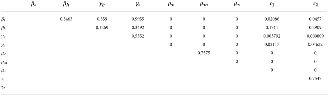
Table 4. Pairwise PRCC comparisons (Unadjusted P-values).
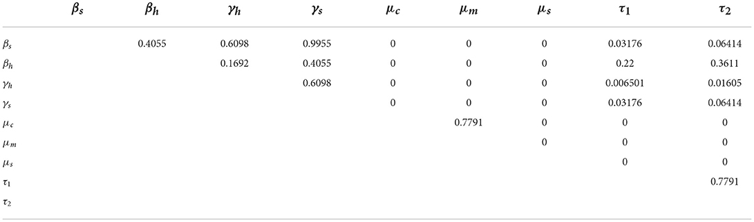
Table 5. Pairwise PRCC comparisons (FDR adjusted P-values).
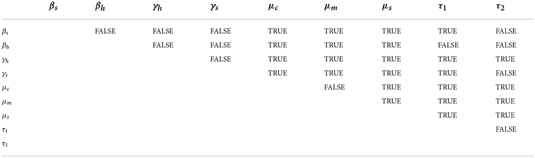
Table 6. Parameters different after FDR adjustment.
The effect of the most sensitive parameters on R0 is presented in Figures 3, 4 as scatter plots to support results in Table 2. These plots show how parameters, βs, γs, γh, τ1, μc, μm, μs, τ2 monotonically increase or decrease R0. The most noticeable result is the scatter plot for snail death μs which is the most sensitive parameter. The sensitivity result reveals that the spread of schistosomiasis infection will be controlled and eradicated in the population if more snails die. If the Miracidia and Cercariae (μm, μc) are cleared within the population, we will observe a reduction in the contact rates of human to Cercariae (βh), snail to Miracidia (βs), probability of egg developing into a Miracidium (τ1) and the density of Cercariae in the environment (τ2).
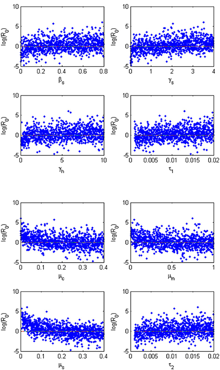
Figure 4. Monte Carlo simulations for the eight parameters that have PRCC values that are significant as evidenced by Table 3. Parameter values were taken from Table 2. Each run consists of 1,000 simulations of randomly drawn parameters.
5. Numerical simulation results
5.1. Time series trajectories
To support the analytical results presented in this paper, we present numerical simulations in the form of time series plots and phase plots on the dynamics of Schistosomiasis. The simulations presented are produced using MATLAB software. Figures 5A,B, present the time series plots for the acute infected class IA(t), chronic infected class, Ich(t), infected animals Ia(t), and infected snails, Ia(t), while varying the snail death rate, μs. The snail death rate, μs is considered for simulation as it is the most sensitive parameter. It is observed that when the death rate of the snail population is increasing, the peak of IA(t), Ich(t), and Ia(t), shifts to the right in a reduced manner. On the other hand, Figures 6A,B present the dynamics of Miracidia, M(t) and Cercariae, C(t). We observe that an increase in the snail death rates leads to a decrease in the population of the Miracidia. Also, the populations of Is(t) and C(t) reduce drastically as the snail population's death rate increases. This indicates that reducing the snail population reduces the time it will take to infect human and mammal populations, including Cercariae that will be cleared in the population. This eventually reduces the number of Schistosomiasis cases within the population.
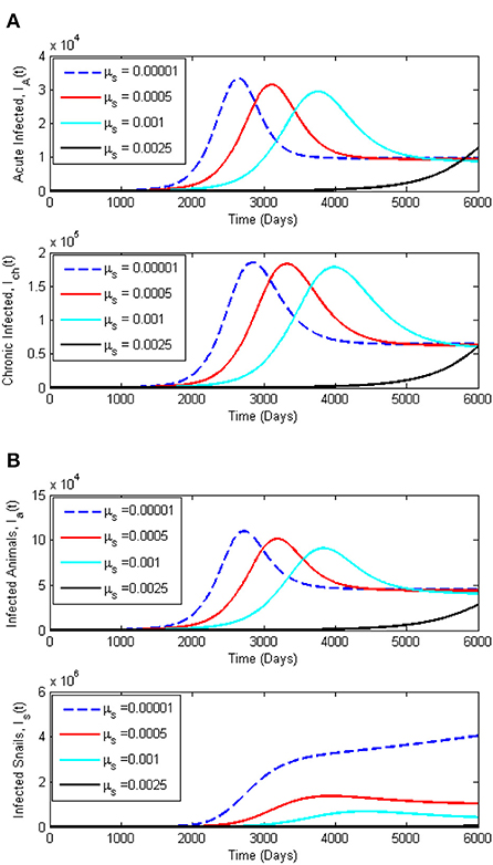
Figure 5. (A) Dynamics of Schistosomiasis infection among the infected human classes, Ia(t) and Ich(t) for varying snail death rate, μs. (B) Dynamics of Schistosomiasis infection among the infected classes, Ia(t) and Is(t) for varying snail death rate, μs. All other parameters for this simulation are given in Table 2.
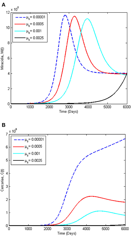
Figure 6. Dynamics of Schistosomiasis infection among: (A) the Miracidia, (M(t)) and (B) the Cercariae classes, (C(t)), for varying snail death rate, μs. All other parameters for this simulation are given in Table 2.
5.2. Phase portraits
Figures 7, 8 present the phase portraits of the infection sub-populations when R0 > 1 and R0 < 1, respectively. When R0 < 1, it can be seen that solutions tend to disease-free equilibrium over time. This means that Schistosomiasis infection can be contained within the population over time provided that R0 < 1. On the other hand when R0 > 1, the solutions lead to an endemic equilibrium as seen by a decrease in the susceptible population and an increase in the infected population. It is also observed that as Miracidia initially increase, Cercariae increases as well and reaches a peak. Thereafter, Miracidia decreases gradually as Cercariae continues to increase. This means that Schistosomiasis infection will persist within the population whenever R0 > 1.
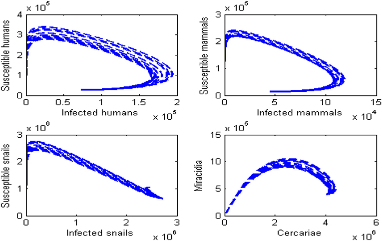
Figure 7. Phase portraits for the dynamics of Schistosomiasis infection when R0 < 1. All other parameters in Table 2.
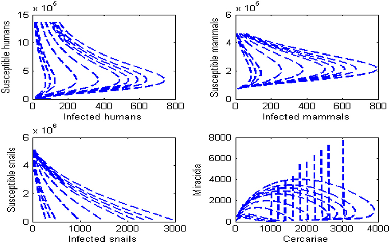
Figure 8. Phase portraits for the dynamics of Schistosomiasis infection when R0 > 1. All other parameters in Table 2.
5.3. Effects of parameters on R0
Using contour plots, Figures 9A,B depict that R0 attains a lower value when the probability of eggs developing into Miracidium is minimal and the snail death rate is high as shown by the contour plot and the 3-D representation. Figure 9C shows R0 vs. varying the natural decay rates of Miracidium, (μm) and Cercariae (μc). It can be seen that if the decay rates are effectively increased, the reproduction number, R0 can be reduced to below one, implying that the disease-free equilibrium can be achieved. The implication of Figures 9A–C is that there is a possibility of approaching a disease-free equilibrium if these parameters are controlled accordingly. However, this may be difficult to attain due to the lack of proper control measures that can simultaneously increase the decay rates. Generally, it can be seen that the control of snails is very important in the reduction of the spread of Schistosomiasis within the population. Therefore, measures need to be put in place so that all breeding areas for snails are identified and dealt with appropriately without harming other aquatic organisms.
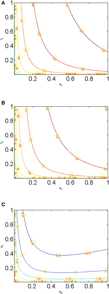
Figure 9. Contour plots showing the effects of (A) τ1 vs. μs (B) τ2 vs. μs (C) μc vs. μm.
6. Conclusion
In this paper, a deterministic mathematical model of transmission dynamics of Schistosomiasis disease that incorporates acute and chronic infected humans is formulated. The main objective of the model is to study the impact of snail control on the dynamics of Schistosomiasis. The model analysis comprised of establishing the invariant region, the positivity of solutions, the existence of disease-free and endemic equilibrium, bifurcation analysis and computation of the basic reproduction number, R0 using the next-generation approach. We proved that whenever R0 < 1, the disease-free equilibrium is globally asymptotically stable, which means that the disease will fizzle out within the population over time. The endemic equilibrium was found to be globally asymptotically stable implying that if not controlled, Schistosomiasis will persist within the population. We also carried out a sensitivity analysis of the parameters governing the basic reproduction number, R0, using the Latin Hypercube Sampling (LHS) scheme-Partial Rank Correlation Coefficient (PRCC) technique. The results of the sensitivity analysis revealed that the spread of schistosomiasis infection can be controlled and eradicated in the population by increasing the natural death rate of the snail population. It also established that there is need to increase the decay rates of Miracidia and Cercariae within the environment by applying a control measure. Therefore, the results of our study effectively conclude that the most effective method to control the transmission dynamics and spread of schistosomiasis disease is by rapidly killing of infected snails and applying control measures that will clear the parasite, miracidia and cercariae, in the environment.
One limitation of our model is that it was not fitted to real-life data. Instead, our model was parameterized using accurate parameter estimates from existing literature on Schistosomiasis dynamics with inclusive heterogeneity in the disease transmission. Secondly, the assumption of mammals could be made specific by considering only cattle in the modeling framework. To bypass this complexity, we carried out a global sensitivity analysis to vary the parameter values and establish the uncertainty in the model parameters. Notwithstanding this limitation, we maintain that our findings remain valid and applicable if followed by policymakers to help eradicate the spread of Schistosomiasis.
Future work may look at an optimal control analysis of the model presented in the presence of different control strategies. The model may also be extended to include infection dynamics in the presence of snail age stratification.
Data availability statement
The original contributions presented in the study are included in the article/supplementary material, further inquiries can be directed to the corresponding author/s.
Author contributions
CM and IO contributed to conception and model formulation of the study. CM, ZC, IO, CC, and FF contributed in the analysis and write-up of sections of the manuscript. All authors contributed to manuscript revision, read, and approved the final version of the manuscript.
Acknowledgments
The authors would like to thank their respective universities and the reviewers for their support toward this manuscript.
Conflict of interest
The authors declare that the research was conducted in the absence of any commercial or financial relationships that could be construed as a potential conflict of interest.
Publisher's note
All claims expressed in this article are solely those of the authors and do not necessarily represent those of their affiliated organizations, or those of the publisher, the editors and the reviewers. Any product that may be evaluated in this article, or claim that may be made by its manufacturer, is not guaranteed or endorsed by the publisher.
References
2. Ross AG, Vickers D, Olds GR, Shah SM, McManus DP. Katayama syndrome. Lancet Infect Dis. (2007) 7:218–24. doi: 10.1016/S1473-3099(07)70053-1
3. Shiff C. The importance of definitive diagnosis in chronic schistosomiasis, with reference to Schistosoma haematobium. J Parasitol Res. (2012) 2012:761269. doi: 10.1155/2012/761269
4. Costa de Limae M, Pocha R, Filhocoura P, Katz N. A 13-years follow-up of treatment and snail control in the endemic area for Schistosoma mansoni in Brazil, incidence of infection and re-infection. Bull World Health Organ. (1993) 71:197–205.
5. Guiro A, Ouaro S, Traore A. Stability analysis of a schistosomiasis model with delays. Adv Differ Equat. (2013) 2013:1–15. doi: 10.1186/1687-1847-2013-303
6. Chen Z, Zou L, Shen D, Zhang W, Ruan S. Mathematical modelling and control of Schistosomiasis in Hubei Province, China. Acta Trop. (2010) 115:119–25. doi: 10.1016/j.actatropica.2010.02.012
7. Sokolow SH, Wood CL, Jones IJ, Swartz SJ, Lopez M, Hsieh MH, et al. Global assessment of schistosomiasis control over the past century shows targeting the snail intermediate host works best. PLoS Neglect Trop Dis. (2016) 10:e0004794. doi: 10.1371/journal.pntd.0004794
8. McCullough F, Gayral P, Duncan J, Christie J. Molluscicides in schistosomiasis control. Bull World Health Organ. (1980) 58:681.
9. Lardans V, Dissous C. Snail control strategies for reduction of schistosomiasis transmission. Parasitol Today. (1998) 14:413–7. doi: 10.1016/S0169-4758(98)01320-9
10. Zhang H, Harvim P, Georgescu P. Preventing the spread of schistosomiasis in Ghana: possible outcomes of integrated optimal control strategies. J Biol Syst. (2017) 25:625–55. doi: 10.1142/S0218339017400058
11. Zhang T, Zhao XQ. Mathematical modeling for schistosomiasis with seasonal influence: a case study in Hubei, China. SIAM J Appl Dyn Syst. (2020) 19:1438–71. doi: 10.1137/19M1280259
12. Bakare E, Nwozo C. Mathematical analysis of malaria-schistosomiasis coinfection model. Epidemiol Res Int. (2016) 2016:3854902. doi: 10.1155/2016/3854902
13. Akanni JO, Olaniyi S, Akinpelu FO. Global asymptotic dynamics of a nonlinear illicit drug use system. J Appl Math Comput. (2021) 66:39–60. doi: 10.1007/s12190-020-01423-7
14. Mustapha UT, Musa SS, Lawan MA, Abba A, Hincal E, Mohammed MD, et al. Mathematical modeling and analysis of schistosomiasis transmission dynamics. Int J Model Simul Sci Comput. (2021) 12:2150021. doi: 10.1142/S1793962321500215
15. Wu YF, Li MT, Sun GQ. Asymptotic analysis of schistosomiasis persistence in models with general functions. J Frankl Instit. (2016) 353:4772–84. doi: 10.1016/j.jfranklin.2016.09.012
16. Ronoh M, Chirove F, Pedro SA, Tchamga MSS, Madubueze CE, Madubueze SC, et al. Modelling the spread of schistosomiasis in humans with environmental transmission. Appl Math Modell. (2021) 95:159–75. doi: 10.1016/j.apm.2021.01.046
17. Qi L, Cui JA, Gao Y, Zhu H. Modeling the schistosomiasis on the islets in Nanjing. Int J Biomath. (2012) 5:1250037. doi: 10.1142/S1793524511001799
18. Abimbade SF, Olaniyi S, Ajala OA. Recurrent malaria dynamics: insight from mathematical modelling. Eur Phys J Plus. (2022) 137:1–16. doi: 10.1140/epjp/s13360-022-02510-3
19. Hethcote HW. The mathematics of infectious diseases. SIAM Rev. (2000) 42:599–653. doi: 10.1137/S0036144500371907
20. Acheampong E, Okyere E, Iddi S, Bonney JH, Asamoah JKK, Wattis JA, et al. Mathematical modelling of earlier stages of COVID-19 transmission dynamics in Ghana. Results Phys. (2022) 34:105193. doi: 10.1016/j.rinp.2022.105193
22. Van den Driessche P, Watmough J. Reproduction numbers and sub-threshold endemic equilibria for compartmental models of disease transmission. Math Biosci. (2002) 180:29–48. doi: 10.1016/S0025-5564(02)00108-6
23. Diekmann O, Heesterbeek JAP, Metz JA. On the definition and the computation of the basic reproduction ratio R 0 in models for infectious diseases in heterogeneous populations. J Math Biol. (1990) 28:365–82. doi: 10.1007/BF00178324
24. Kim JH, Su W, Song YJ. On stability of a polynomial. J Appl Math Inform. (2018) 36:231–6. doi: 10.14317/jami.2018.231
25. Heffernan JM, Smith RJ, Wahl LM. Perspectives on the basic reproductive ratio. J R Soc Interface. (2005) 2:281–93. doi: 10.1098/rsif.2005.0042
26. Chavez CC, Feng Z, Huang W. On the computation of R0 and its role on global stability. In: Castillo-Chavex C Blower S Driessche P Kirschner D Yakubu A-A, editors. Mathematical Approaches for Emerging and Re-emerging Infection Diseases: An Introduction, Vol. 125. New York, NY: Springer (2002) p. 31–65. doi: 10.1007/978-1-4757-3667-0_13
27. Castillo-Chavez C, Song B. Dynamical models of tuberculosis and their applications. Math Biosci Eng. (2004) 1:361. doi: 10.3934/mbe.2004.1.361
28. Shuai Z, van den Driessche P. Global stability of infectious disease models using Lyapunov functions. SIAM J Appl Math. (2013) 73:1513–32. doi: 10.1137/120876642
29. Kalinda C, Mushayabasa S, Chimbari MJ, Mukaratirwa S. Optimal control applied to a temperature dependent schistosomiasis model. Biosystems. (2019) 175:47–56. doi: 10.1016/j.biosystems.2018.11.008
30. Feng Z, Eppert A, Milner FA, Minchella D. Estimation of parameters governing the transmission dynamics of schistosomes. Appl Math Lett. (2004) 17:1105–12. doi: 10.1016/j.aml.2004.02.002
31. Chiyaka ET, GARIRA W. Mathematical analysis of the transmission dynamics of schistosomiasis in the human-snail hosts. J Biol Syst. (2009) 17:397–423. doi: 10.1142/S0218339009002910
32. Abokwara A, Madubueze CE. The role of non-pharmacological interventions on the dynamics of schistosomiasis. J Math Fund Sci. (2021) 53:243–260. doi: 10.5614/j.math.fund.sci.2021.53.2.6
33. Kanyi E, Afolabi AS, Onyango NO. Mathematical modeling and analysis of transmission dynamics and control of schistosomiasis. J Appl Math. (2021) 2021:6653796. doi: 10.1155/2021/6653796
34. Mangal TD, Paterson S, Fenton A. Predicting the impact of long-term temperature changes on the epidemiology and control of schistosomiasis: a mechanistic model. PLoS ONE. (2008) 3:e1438. doi: 10.1371/journal.pone.0001438
35. Li Y, Teng Z, Ruan S, Li M, Feng X. A mathematical model for the seasonal transmission of schistosomiasis in the lake and marshland regions of China. Math Biosci Eng. (2017) 14:1279. doi: 10.3934/mbe.2017066
36. Xiang J, Chen H, Ishikawa H. A mathematical model for the transmission of Schistosoma japonicum in consideration of seasonal water level fluctuations of Poyang Lake in Jiangxi, China. Parasitol Int. (2013) 62:118–26. doi: 10.1016/j.parint.2012.10.004
37. Gao SJ, Cao HH, He YY, Liu YJ, Zhang XY, Yang GJ, et al. The basic reproductive ratio of Barbour's two-host schistosomiasis model with seasonal fluctuations. Parasites Vectors. (2017) 10:1–9. doi: 10.1186/s13071-017-1983-1
38. Ding C, Qiu Z, Zhu H. Multi-host transmission dynamics of schistosomiasis and its optimal control. Math Biosci Eng. (2015) 12:983. doi: 10.3934/mbe.2015.12.983
39. Blower SM, Dowlatabadi H. Sensitivity and uncertainty analysis of complex models of disease transmission: an HIV model, as an example. Int Stat Rev. (1994) 62:229–43. doi: 10.2307/1403510
40. Herdicho FF, Chukwu W, Tasman H. An optimal control of malaria transmission model with mosquito seasonal factor. Results Phys. (2021) 25:104238. doi: 10.1016/j.rinp.2021.104238
41. Chukwu C, Nyabadza F. A theoretical model of listeriosis driven by cross contamination of ready-to-eat food products. Int J Math Math Sci. (2020) 2020:9207403. doi: 10.1155/2020/9207403
42. Chazuka Z, Moremedi GM. In-host dynamics of the human papillomavirus (HPV) in the presence of immune response. In:Mondaini RP, , editor. Trends in Biomathematics: Chaos and Control in Epidemics, Ecosystems, and Cells: Selected Works from the 20th BIOMAT Consortium Lectures, Rio de Janeiro, Brazil, 2020. Cham: Springer (2021). p. 79–97. doi: 10.1007/978-3-030-73241-7_6
43. Chukwu CW, Mushanyu J, Juga ML, Fatmawathi. A mathematical model for co-dynamics of listeriosis and bacterial meningitis diseases. Commun Math Biol Neurosci. (2020) 2020:ID83.
44. Madubueze CE, Chazuka Z. An optimal control model for the transmission dynamics of Lassa fever. Res Squ. [Preprint]. doi: 10.21203/rs.3.rs-1513399/v1
Keywords: schistosomiasis, heterogeneous host, mathematical analysis, sensitivity analysis, global stability
Citation: Madubueze CE, Chazuka Z, Onwubuya IO, Fatmawati F and Chukwu CW (2022) On the mathematical modeling of schistosomiasis transmission dynamics with heterogeneous intermediate host. Front. Appl. Math. Stat. 8:1020161. doi: 10.3389/fams.2022.1020161
Received: 15 August 2022; Accepted: 23 September 2022;
Published: 13 October 2022.
Edited by:
Samson Olaniyi, Ladoke Akintola University of Technology, NigeriaReviewed by:
Stephen E. Moore, University of Cape Coast, GhanaEric Okyere, University of Energy and Natural Resources, Ghana
Copyright © 2022 Madubueze, Chazuka, Onwubuya, Fatmawati and Chukwu. This is an open-access article distributed under the terms of the Creative Commons Attribution License (CC BY). The use, distribution or reproduction in other forums is permitted, provided the original author(s) and the copyright owner(s) are credited and that the original publication in this journal is cited, in accordance with accepted academic practice. No use, distribution or reproduction is permitted which does not comply with these terms.
*Correspondence: Chinwendu E. Madubueze, ce.madubueze@gmail.com