Noise and solar-wind/magnetosphere coupling studies: Data

1 Introduction

Correlative-type data studies comparing the behavior of the magnetosphere-ionosphere system to the behavior of the solar wind are performed 1) to determine the solar-wind variables that control magnetospheric activity and 2) to determine or confirm the physics of solar-wind/magnetosphere coupling. Often a goal is to find the most accurate solar-wind driver function (coupling function) to describe magnetospheric activity in terms of solar-wind parameters [e.g., Newell et al., 2007; 2008; Borovsky, 2014; McPherron et al., 2015; Lockwood and McWilliams, 2021]. There is hope that this best driver function describes the physics of solar-wind/magnetosphere coupling, but see the discussion in Borovsky (2021). It is known that noise in the data reduces the quality of a fit of one data set to another data set (Spearman, 1904; Bock and Petersen, 1975; Liu, 1988; Hutcheon et al., 2010). This is true for the magnetospheric and solar-wind data sets (Sivadas and Sibeck, 2022). Using artificial data sets Borovsky (2022a) demonstrated that noise (error) in the solar-wind measurements can also change the functional form of best-fit solar-wind driver functions when fitting solar-wind data to geomagnetic indices. Note that Borovsky (2022a) found that adding noise to geomagnetic indices does not change the best-fit formula for the solar-wind driving of that index, the added noise just reduces the solar-wind/magnetosphere correlation coefficient.

We know that the real solar-wind data used for such coupling studies has noise (errors), mostly owed to the use of solar-wind monitors located far from the Earth at L1 (Sandahl et al., 1996; Ashour-Abdalla et al., 2008; Walsh et al., 2019; Burkholder et al., 2020; Borovsky, 2020a, 2022b; Lockwood, 2022; Sivadas and Sibeck, 2022). The basic error is incorrect values caused by the fact that the solar wind that hits an L1 monitor is typically not the solar wind that hits the Earth (Walsh et al., 2019; Burkholder et al., 2020; Borovsky, 2020a, 2022b). The error this causes is incorrect values, not propagation-time errors. If that measurement noise could be removed, more-valuable best-fit driver functions, in the sense that they may better describe the physics of coupling, could be obtained.

In this report the effects of noise in the real solar-wind data will be explored. Controlled noise will be added to the solar-wind data and the effect of that noise on best-fit solar-wind drivers will be analyzed. To explore the effects of noise, noise will be added to the solar-wind data in two simple, controlled fashions: 1) random values extracted from Gaussian distributions will b added to all values in the solar-wind time series or 2) a fraction of the time-series values will be completely replace with other values. Arguments extrapolating backward to remove noise in the solar-wind data will be made and data from the years in which the near-Earth solar-wind monitor IMP-8 operated will be explored.

2 Data sets

A commonly used solar-wind driver function that was obtained as a best fit to geomagnetic data is the “Newell function” v_sw^4/3B_⊥^2/3sin^8/3(θ_clock/2) (Newell et al., 2007), where v_sw is the solar-wind speed, B_⊥ is the magnitude of the component of the solar-wind magnetic field that is perpendicular to the Sun-Earth line, and θ_clock = Arccos(B_z/(B_y²+B_z²)^1/2) is the (GSM) clock angle of the solar-wind magnetic field relative to the Earth’s magnetic dipole. Here we will form best-fit driver functions D = v_sw^aB_sw^bsin^c(θ_clock/2) where the exponents a, b, and c are optimized so that D has the largest Pearson linear correlation coefficient with various time-lagged geomagnetic indices. For the solar-wind data 1-h averages in the OMNI2 data set (King and Papitashvili, 2005) for the years 1995–2018 are used. In making hourly averaged values of sin(θ_clock/2), hourly averaged values of B_y and B_z from OMNI2 are used: Lockwood and McWilliams (2021) and Lockwood (2022) point out that creating high-time-resolution values of sin(θ_clock/2) and then making an hourly average of those sin(θ_clock/2) values (combine-then-average) would be a superior method. Statistically comparing the results of the two methods finds that the distribution of θ_clock values obtained have very similar mean values, but the calculate from high-resolution and then average yields a distribution with many fewer occurrences near 0^o clock angle and many fewer occurrences near 180^o clock angle. Thus for a given functional form of a driver function, the combine-then-average method yields far fewer cases of extremely weak driving and far fewer cases of extremely strong driving (as measured by the magnitude of the driver function) than does the calculating from averaged values of B_y and B_z (average-then-combine).

In the data analysis each of the three solar-wind variables v_sw, B_sw, and sin(θ_clock/2) is “standardized” by first subtracting the mean value from every value and then by dividing every value by the standard deviation of the distribution of values. Each standardized solar-wind variable has a mean value of zero and a standard deviation of unity. Then Gaussian noise (Gaussianly distributed random numbers) is added to the standardized solar-wind variables in a number of ways: adding noise to only one solar-wind variable or adding noise to all three solar-wind variables. The amplitude of the noise is varied. When the amplitude of the noise is “1” the noise has the same standard deviation as the variable.

The years 1995–2018 are chosen for two reasons. First, we will be using at times the Hp60 index, which is only available since 1995. Hp60 is a 60-min-resolution version of the 3-hr-resolution Kp index, available at ftp://ftp.gfz-potsdam.de/pub/home/obs/Hpo. Second, as part of this project we want to compare the results from using solar-wind data at L1 with solar wind measurements closer to the Earth from the IMP-8 spacecraft (Feldman et al., 1978; Butler, 1980): the OMNI2 data beginning in 1995 is almost exclusively from L1 with the WIND spacecraft launched in 1995 and the ACE spacecraft launched in 1998.

The geomagnetic indices that will be used are the following, all at 1-h time resolution. The time lags given to each index comes from optimal lags found in prior solar-wind-coupling studies. The auroral-electrojet indices AE, AL, and AU (and their SuperMag equivalents SME, SML, and SMU) measure the peak intensity of high-latitude ionospheric current in the auroral electrojet: they are considered to be an indicator of the intensity of auroral activity (Goertz et al., 1993) and total Joule dissipation in the ionosphere (Baumjohann, 1986). They are utilized with a 1-h time lag from the OMNI solar wind data. The polar-cap index PC is a measure of the intensity of ionospheric current flowing across the northern polar cap: it is related to the intensity of polar-cap anti-Sunward convection (Stauning, 2013) and the cross-polar-cap potential (Ridley and Kihn, 2004). It is utilized with a 0-h time lag from the OMNI solar wind data. The Kp, Hp60, and Ap60 indices measure the strength of mid-latitude ionospheric currents around the Earth: they are a measure of the strength of magnetospheric convection (Thomsen, 2004). They are utilized with a 1-h time lag from the OMNI solar wind data. The Dst current measures an equatorial magnetic-field perturbation: that perturbation is related to the plasma pressure in the dipolar portions of the magnetosphere (Dessler and Parker, 1959; Sckopke, 1966; Liemohn et al., 2001), but it is also perturbed by the Chapman-Ferraro current at the dayside magnetosphere (Su and Konradi, 1975; Siscoe et al., 2005) and by the cross-tail current in the magnetotail (Ohtani et al., 2001; Borovsky and Denton, 2010). It is utilized with a 2-h time lag from the OMNI solar wind data.

3 The data studies

In Figure 1 the 1-hr-lagged (from the solar wind) SuperMAG auroral electrojet index SME₁ is studied. SME measures high-latitude auroral-zone ionospheric currents using 80-or-more ground-based magnetometers [the SuperMAG network (Bergin et al., 2020)], wheras the older AE index makes the same measurement using ∼12 magnetometers. In the top three panels the values of the three exponents a, b, and c of D = v_sw^aB_sw^bsin^c(θ_clock/2) are plotted vertically as a function of the amplitude of the added noise horizontally: a (v_sw) is plotted in red, b (B_sw) is plotted in blue, and c [sin(θ_clock/2)] is plotted in green. For the solid curves with round points noise is added only to v_sw, for the solid curves with triangle points noise is added only to B_sw, for the thick solid curves with square points noise is added only to sin(θ_clock/2), and for the dashed curves noise is added to all three of the solar-wind variables. In the bottom panel of Figure 1 the Pearson linear correlation coefficient between D and SME₁ is plotted as a function of the amplitude of the added noise.

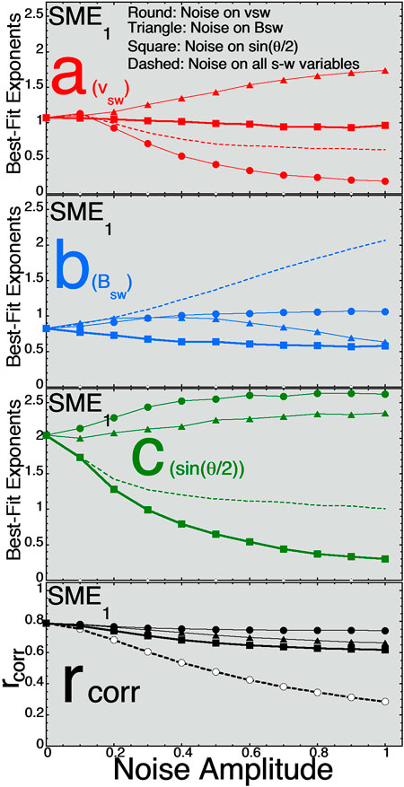
FIGURE 1. For best fits to the 1-hr-lagged SME₁ index the three exponents (A) (red, top panel), (B) (blue, second panel), and (C) (green, third panel) are plotted as functions of the amplitude of the Gaussian noise added to the three solar-wind variables. In the bottom panel the Pearson linear correlation coefficient between D = v_sw^aB_sw^bsin^c(θ_clock/2) and SME₁ is plotted as a function of the amplitude of the added noise.

Note that Newell et al., 2007 used B_⊥ = (B_y²+B_z²)^1/2 and used multiple hours of solar-wind data in the fitting: here we are using B_sw = (B_x²+B_y²+B_z²)^1/2 and using only a single hour of solar-wind data in the fitting.

SME is a “high-latitude” index measuring the strength of high-latitude magnetosphere-ionosphere currents. In creating plots similar to Figure 1 for other high-latitude indices (AE, AU, AL, and PCI, and the SuperMAG versions of the AL and AU indices called SML and SMU) one finds very similar trends on the plots, with the exponent c on sin(θ_clock/2) being the largest of the three exponents.

Figure 2 plots the best-fit exponents a, b, and c for D = v_sw^aB_sw^bsin^c(θ_clock/2) for the 1-hr-lagged Hp60₁ index. Hp60 is a convection-strength index (as is Kp, Ap, and MBI) (Thomsen, 2004) reacting to the strength of magnetospheric convection. These convection indices do not focus on the rapidly changing clock angle of the solar wind sin(θ_clock/2) and so the c exponent for sin(θ_clock/2) is small for these convective indices.

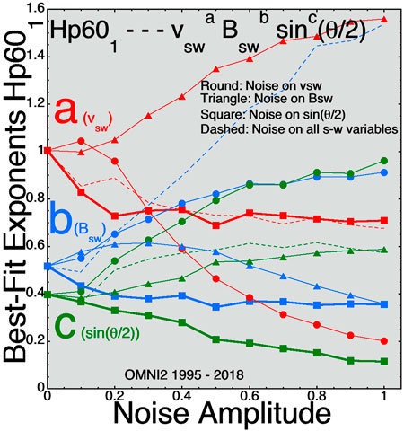
FIGURE 2. For best fits to the 1-hr-lagged Hp60₁ index the three exponents (A) (red), (B) (blue), and (C) (green) are plotted as functions of the amplitude of the Gaussian noise added to the three solar-wind variables.

Figure 3 plots the best fit exponents a, b, and c for D = v_sw^aB_sw^bsin^c(θ_clock/2) for the 2-hr-lagged Dst index. Dst measures mostly the pressure (diamagnetic currents) of plasma in the inner magnetosphere. The 2-h lag was chosen because that was found to be optimal in prior solar-wind/magnetosphere coupling studies using 1-h averaged data [e.g. Borovsky, 2020b]. Like the convection indices, the exponent c of sin(θ_clock/2) is weak.

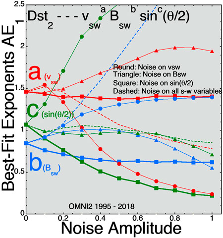
FIGURE 3. For best fits to the 2-hr-lagged Dst₂ index the three exponents (A) (red), (B) (blue), and (C) (green) are plotted as functions of the amplitude of the Gaussian noise added to the three solar-wind variables.

Examining a number of these plots for various geomagnetic indices some trends can be seen. 1) Increasing the noise on v_sw reduces the magnitude of the exponent a on v_sw. 2) Increasing the noise on sin(θ_clock/2) reduces the magnitude of the exponent c on sin(θ_clock/2). 3) Increasing the noise on B_sw at first increases the magnitude of the exponent b on B_sw and then as the noise amplitude becomes large it decreases the magnitude of the exponent b. 4) Increasing the noise on v_sw tends to raise the magnitudes of the exponents b and c on B_sw and sin(θ_clock/2). 5) Increasing the noise on B_sw tends to raise the magnitudes of the exponents a and c on v_sw and sin(θ_clock/2). 6) Increasing the noise on sin(θ_clock/2) tends to lower the magnitude of all three exponents a, b, and c. Note that there are exceptions to these trends.

Examining plots similar to those of Figures 1–3 for a number of geomagnetic indices, the trend in each of the exponents a, b, and c are noted in Table 1 as noise is added to the OMNI2 solar-wind variables v_sw, B_sw, and sin(θ_clock/2). An upward arrow in Table 1 indicates that the value of the exponent increases with increasing noise amplitude and a downward arrow indicates that the value of the exponent decreases with increasing noise amplitude.

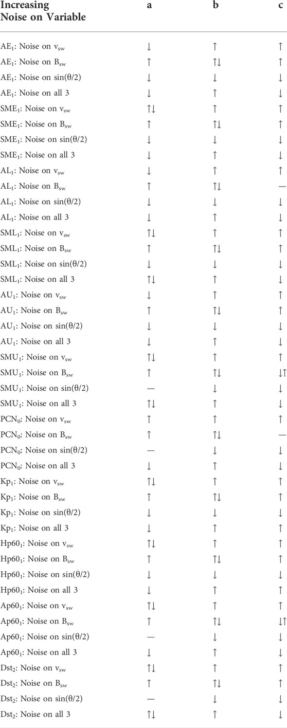
TABLE 1. An increase (↑) or a decrease (↓) to the three exponents a, b, and c of D = v_sw^aB_sw^bsin^c(θ_clock/2) are noted as Gaussian random noise is added to the OMNI2 solar-wind variables for the years 1995–2018.

4 Extrapolating backward to remove or reduce the solar-wind noise

Looking at the trends in the changes of the a, b, and c exponents of D = v_sw^aB_sw^bsin^c(θ_clock/2) with increasing added noise, one might guess that extrapolating the curves in the plots of Figures 1–3 back to values of noise < 0 might represent the better values of the exponents a, b, and c in the presence of less solar-wind noise (less error). Figure 4 plots the temporal autocorrelation functions of the three variables v_sw (red curve), B_sw (blue curve), and sin(θ_clock/2) (green curve) obtained from 64-s-resolution data from ACE SWEPAM (McComas et al., 1998) and ACE MAG (Smith et al., 1998) for the year 2006. (The year 2006 is in the late declining phase with mild high-speed streams and with a nice mix of solar-wind plasma types [cf. Xu and Borovsky, 2015].) The autocorrelation times (using the 1/e method) in Figure 4 are about 43.9 h for v_sw, 15.3 h for B_sw, and 53 min for sin(θ_clock/2). The temporal autocorrelation function represents the spatial structure of the solar-wind plasma and magnetic field advected past the measuring spacecraft. The spatial structure of the variable sin(θ_clock/2) in the solar wind is much smaller than the spatial structure of the variables B_sw and v_sw, hence the much shorter autocorrelation time for sin(θ_clock/2) [See also Lockwood and McWilliams (2021)]. One problem with a solar-wind monitor for Earth at L1 is that the solar wind that hits the L1 monitor is not the same solar wind that hits the Earth (Sandahl et al., 1996; Ashour-Abdalla et al., 2008; Walsh et al., 2019; Burkholder et al., 2020; Borovsky, 2020a): the monitored solar-wind streamline often misses the Earth by 10s of R_E typically passing on the duskward side of the magnetosphere (Borovsky, 2022b). Contributing factors for this miss are 1) the solar-wind flow is not radial [the direction fluctuates by about ±5° plus there is a systematic dawn-dusk offset to the average flow vector (Nemecek et a., 2020a)] 2) there is a duskward aberration to the flow caused by the Earth’s motion around the Sun (Fairfield, 1993), and 3) the solar-wind structure moves away from the Sun faster than the plasma wind with a velocity vector relative to the plasma that is in the Parker-spiral direction (Borovsky, 2020c; Nemecek et al., 2020b). This L1 error is much more critical for the smaller-structured sin(θ_clock/2) than it is for v_sw or B_sw. Hence the thick solid curves with the square points in Figures 1–3 that add noise only to sin(θ_clock/2) are the most important to think about and extrapolate backward.

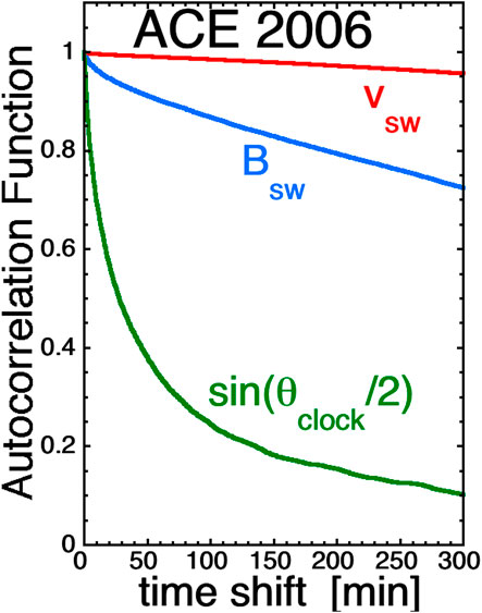
FIGURE 4. Autocorrelation functions for the three solar-wind variables v_sw (red), B_sw (blue), and sin(θ_clock/2) (green) calculated using 64-s measurements from ACE for the year 2006.

For the high-latitude-current indices AE, AU, AL, SME, SMU, SML, and PCI the exponent c on sin(θ_clock/2) is the largest of the three exponents and also undergoes the most-significant change (reduction) as noise is added to the sin(θ_clock/2) values in the data set (cf. Figure 1). Extrapolating to negative values of noise in the thick solid curves of Figures 1–3 would increase the magnitude of the c exponent: the extrapolation would not change a (for v_sw) or b (for B_sw) significantly. For the magnetospheric convection index Hp60₁ extrapolating backward to noise values less than zero on sin(θ_clock/2) in Figure 2 (thick curve with square points) would increase the a exponent (on v_sw) the most and also increase the b (on B_sw) and c [on sin(θ_clock/2)] exponents.

One might guess that by using the times when the nearer-to-Earth solar-wind monitor IMP-8 (Feldman et al., 1978; Butler, 1980) was used in the OMNI2 data set, these extrapolations to lower noise could be confirmed. Unfortunately, it will be seen that this is not the case. In Table 2 the best-fit values for the exponents a, b, and c for five geomagnetic indices are listed for the hours when IMP-8 solar-wind measurements were incorporated into OMNI2 (with most of the IMP-8 data incorporated in the years 1975–1994). The best-fit values of a, b, and c are also listed in Table 2 for the 1995–2018 OMNI2 data. The changes in a, b, and c predicted by extrapolation of the 1995–2018 data (cf. Table 1) are noted, and the observed changes in a, b, and c from the 1995–2018 data to the IMP-8 data are noted in Table 2. (Note that these expected changes are opposite to the arrows in Table 1: the arrows are the direction when noise is added and the “expected” change is the expectation for reduction of noise.) As can be seen in Table 2, the changes observed by using IMP-8 are in poor agreement with the extrapolation-predicted changes from the 1995–2018 added-noise calculations: eight times there is agreement and seven times there is disagreement. Note that the change in the exponent b on B_sw is wrong for all five cases.

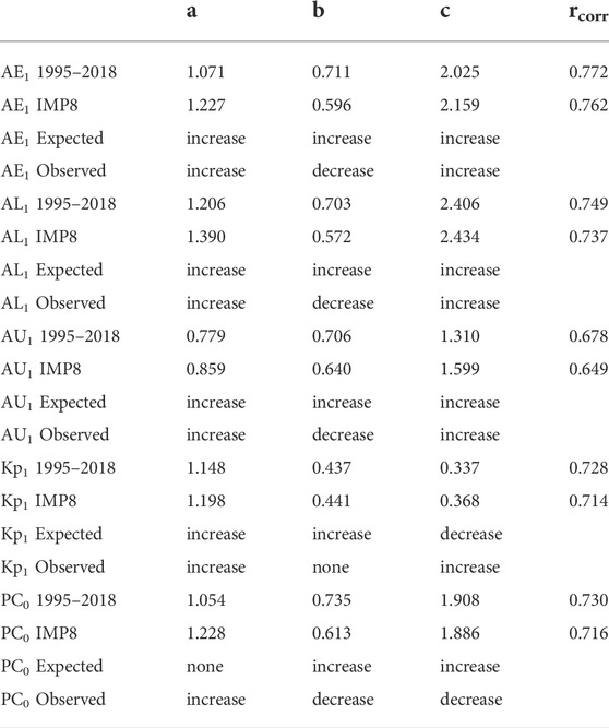
TABLE 2. For five different geomagnetic indices the best-fit exponents a, b, and c of the solar-wind driver D = v_sw^aB_sw^bsin^c(θ_clock/2) are listed for the 1995–2018 OMNI2 solar-wind data and for the OMNI2 data that utilized measurements from IMP-8. The expected change in the a, b, and c exponents if there were a reduction of noise on sin(θ_clock/2) and the observed change in the exponents a, b, and c (from Table 1) are listed.

The bottom panel of Figure 5 plots the best-fit a, b, and c exponents to AE₁ in four-year blocks of OMNI2 solar-wind data from 1995–2018. As can be seen, the values of these best-fit exponents change from data subset to data subset. In the top panel of Figure 5 the 27-days-averaged sunspot number R is plotted. The temporal changes in the exponents seen in the bottom panel might be owed to solar-cycle-type variations in the solar-wind properties and/or to solar-wind spacecraft differences from year to year. As a comparison for Figure 5, Figure 6 looks at the best-fit a, b, and c exponents for AE₁ when the 1995–2018 OMNI2 data is randomized in time and binned into 10 subsets, each containing data from the full years 1995–2018. When the data is mixed in time (Figure 6) it results in much smaller variations in the best-fit exponents a, b, and c from data subset to data subset, supporting the idea that there are variances caused by spacecraft differences and by year-by-year solar-cycle differences in the wind. The variances in a, b, and c in Figure 5 are large, and so the choosing of IMP-8 data in a finite set of years could result in variations of a, b, and c that are more-significant than the noise-reduction changes. Hence the hope that using IMP-8 to reduce the noise and improve the a, b, and c values is not so straightforward: moving to IMP-8 from the 1995–2018 data set does not always move the a, b, and c values in the expected direction and changing eras (years) and spacecraft results in changes to the behavior of the a, b, and c values. A question is which of these year-to-year changes in a, b, and c (e.g. Figure 5) are better and which are worse in terms of finding a driver function that describes the physics of the solar wind coupling to the Earth; as discussed in Borovsky (2021) there are math-versus-physics reasons why a driver function has a good correlation with the Earth.

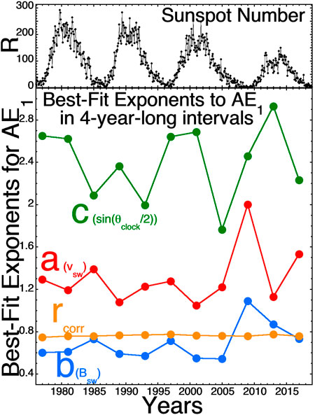
FIGURE 5. (top panel) For the years 1995–2008 the 27-days-averaged sunspot number is plotted. (bottom panel) The best-fit (A) (red), (B) (blue), and (C) (green) exponents for AE₁ are calculated in four-year blocks of OMNI2 solar-wind data from 1995–2018. For each four-year data block the Pearson linear correlation coefficient between D and AE₁ is plotted in orange.

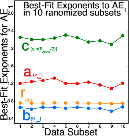
FIGURE 6. The best-fit (A) (red), (B) (blue), and (C) (green) exponents for AE₁ are plotted when the 1995–2018 OMNI2 data is randomized in time and binned into 10 subsets, each of which containing data from the full years 1995–2018. The Pearson linear correlation coefficient for each subset is plotted in orange.

5 Discussion

This report explored expectations for solar-wind noise reduction by looking at the trends that resulted from adding Gaussian noise to solar-wind data. Extrapolating those added-noise trends backward yielded predictions for noise-reduction changes to the exponents a, b, and c of best-fit connections between the solar-wind driver function D = v_sw^aB_sw^bsin^c(θ_clock/2) and various geomagnetic indices. Going from L1 solar-wind data to near-Earth IMP-8 solar-wind data, the observed changes in the exponents a, b, and c of the best-fit formula D = v_sw^aB_sw^bsin^c(θ_clock/2) did not show good agreement with the expected noise-reduction changes. Looking at year-to-year changes in the a, b, and c exponents for the best-fit formula found that these year-to-year changes were large: hence different parts of the solar cycle and/or using different spacecraft to monitor the solar wind results in large changes that may overwhelm observation of the desired noise-reduction changes.

One issue with the methodology used here is the addition of Gaussian noise (random numbers with Gaussian distributions) to the OMNI2 solar-wind variables. The main error with solar-wind monitors at L1 is that the solar wind that hits a monitoring spacecraft at L1 is not the solar wind that hits the Earth. Hence the real error in the solar-wind data for Earth is not random noise on all solar-wind values, rather that some of the values are completely wrong. Adding noise, for instance, by replacing a fraction of the sin(θ_clock/2) values in the time series with completely different values of sin(θ_clock/2) may be a more-realistic way to emulate the L1 errors in the solar-wind measurements. This is explored in Figures 7–9 where the best-fit exponents a, b, and c are plotted as a function of the fraction of the solar-wind time-series values that are replaced with different values. Comparing Figure 7 with Figure 1 (fits to SuperMAG SME₁), Figure 8 with Figure 2 (Fits to Hp60₁), and Figure 9 with Figure 3 (fits to Dst₂), it is seen that the trends in the changes of the exponents a, b, and c with increasing noise (either increasing the amplitude of added Gaussian noise or increasing the fraction of time-series values replaced) are quite similar. Between these three pairs of plots there are no contradictions where one method leads to an increase in an exponent and the other leads to a decrease in that exponent. There are a few cases where the Gaussian-noise method leads to an increase or a decrease of an exponent while the replacement method shows no change in that exponent.

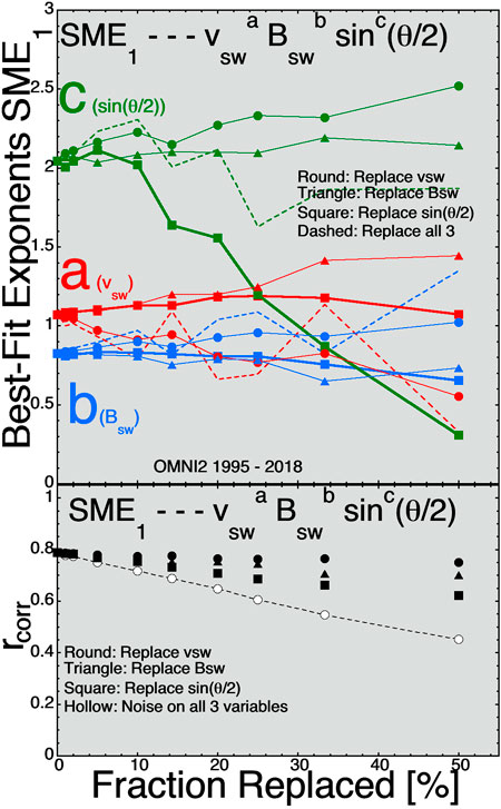
FIGURE 7. For best fits to the 1-hr-lagged SME₁ index the three exponents (A) (red), (B) (blue), and (C) (green) are plotted in the top panel as functions of the fraction of time-series values replaced for three solar-wind variables. In the bottom panel the Pearson linear correlation coefficient between D and SME₁ is plotted as a function of the fraction replaced.

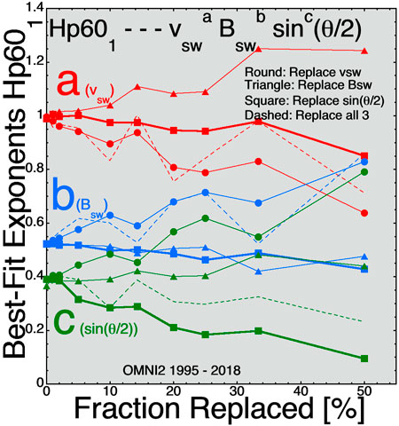
FIGURE 8. For best fits to the 1-hr-lagged Hp60₁ index the three exponents (A) (red), (B) (blue), and (C) (green) are plotted as functions of the fraction of time-series values replaced for three solar-wind variables.

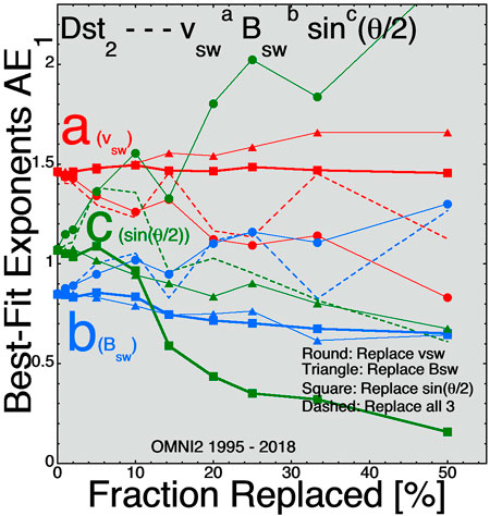
FIGURE 9. For best fits to the 2-hr-lagged Dst₂ index the three exponents (A) (red), (B) (blue), and (C) (green) are plotted as functions of the fraction of time-series values replaced for three solar-wind variables.

For 1-hour-averaged data, the L1 error most likely does not result in the whole hour being incorrect, but just part of the hour being incorrect. A hybrid methodology to add noise might try adding random noise (for the fraction of the hour being wrong) to only some of the hourly solar-wind data points. Since the two methods 1) adding noise to all solar-wind data points and 2) replacing a fraction of the data points both yielded similar results, one might guess that adding noise to a fraction of the data points will also yield similar results.

The analysis of this study using IMP-8 data found difficulty in demonstrating that near-Earth monitoring yields more-accurate solar-wind measurements for Earth, although there have been several studies estimating of the solar-wind errors between L1 and Earth (Crooker et al., 1982; Ridley, 2000; Weimer et al., 2002; Mailyan et al., 2008; Case and Wild, 2012). That is not to say that this study does not recommend fielding near-Earth solar-wind monitors in future. It is an intellectual certainty that better solar-wind-monitor measurements with truer values of what is hitting the Earth will result in better future data studies of solar-wind/magnetosphere interactions. A study to optimize monitors for solar-wind/magnetosphere interaction science is needed. One possibility is multiple spacecraft in IMP-type circular orbits (r ∼ 30 R_E) (Feldman et al., 1978; Butler, 1980) where at least one spacecraft would always be in the near-Earth upstream solar wind.

Data availability statement

Publicly available datasets were analyzed in this study. This data can be found here: https://omniweb.gsfc.nasa.gov.

Author contributions

The author confirms being the sole contributor of this work and has approved it for publication.

Funding

JB was supported at the Space Science Institute by the NSF GEM Program via grant AGS-2027569 and by the NASA HERMES Interdisciplinary Science Program via grant 80NSSC21K1406.

Acknowledgments

The author thanks Mike Lockwood and Nithin Sivadas for useful conversations. The author also acknowledges GFZ Potsdam for the Hp60 index, which is available at ftp://ftp.gfz-potsdam.de/pub/home/obs/Hpo, and the author acknowledges the SuperMAG team, where the SuperMAG auroral-electrojet indices are available at http://supermag.jhuapl.edu/indices.

Conflict of interest

The authors declare that the research was conducted in the absence of any commercial or financial relationships that could be construed as a potential conflict of interest.

Publisher’s note

All claims expressed in this article are solely those of the authors and do not necessarily represent those of their affiliated organizations, or those of the publisher, the editors and the reviewers. Any product that may be evaluated in this article, or claim that may be made by its manufacturer, is not guaranteed or endorsed by the publisher.

References

Ashour-Abdalla, M., Walker, R. J., Peroomian, V., and El-Alaoui, M. (2008). On the importance of accurate solar wind measurements for studying magnetospheric dynamics. J. Geophys. Res. 113, A08204. doi:10.1029/2007ja012785
Baumjohann, W. (1986). Merits and limitations of the use of geomagnetic indices in solar wind-magnetosphere coupling studies, in Solar wind-magnetosphere coupling, Y. Kamide, and J. A. Slavin (eds.), p. 3, Terra Scientific, Tokyo.
Bergin, A., Chapman, S. C., and Gjerloev, J. W. (2020). A E , DST , and their SuperMAG counterparts: The effect of improved spatial resolution in geomagnetic indices. J. Geophys. Res. Space Phys. 125, e2020JA027828. doi:10.1029/2020ja027828
Bock, R. D., and Petersen, A. C. (1975). A multivariate correction for attenuation. Biometrika 62, 673–678. doi:10.1093/biomet/62.3.673
Borovsky, J. E. (2020b). A survey of geomagnetic and plasma time lags in the solar-wind-driven magnetosphere of Earth. J. Atmos. Sol. Terr. Phys. 208, 105376. doi:10.1016/j.jastp.2020.105376
Borovsky, J. E. (2014). Canonical correlation analysis of the combined solar-wind and geomagnetic-index data sets. J. Geophys. Res. Space Phys. 119, 5364–5381. doi:10.1002/2013ja019607
Borovsky, J. E., and Denton, M. H. (2010). The magnetic field at geosynchronous orbit during high-speed-stream-driven storms: Connections to the solar wind, the plasma sheet, and the outer electron radiation belt. J. Geophys. Res. 2010, 115A08217. doi:10.1029/2009JA015116
Borovsky, J. E. (2022a). Noise, regression dilution bias, and solar-wind/magnetosphere coupling studies. Front. Astron. Space Sci. 9, 867282. doi:10.3389/fspas.2022.867282
Borovsky, J. E. (2020c). On the motion of the heliospheric magnetic structure through the solar wind plasma. J. Geophys. Res. Space Phys. 125, e2019JA027377. doi:10.1029/2019JA027377
Borovsky, J. E. (2021). Perspective: Is our understanding of solar-wind/magnetosphere coupling satisfactory? Front. Astron. Space Sci. 8, 634073. doi:10.3389/fspas.2021.634073
Borovsky, J. E. (2022b). The triple dusk-dawn aberration of the solar wind at Earth. Front. Astron. Space Sci. 9, 917163. doi:10.3389/fspas.2022.917163
Borovsky, J. E. (2020a). What magnetospheric and ionospheric researchers should know about the solar wind. J. Atmos. Sol. Terr. Phys. 204, 105271. doi:10.1016/j.jastp.2020.105271
Burkholder, B. L., Nykyri, K., and Ma, X. (2020). Use of the L1 constellation as a multispacecraft solar wind monitor. JGR. Space Phys. 125, e2020JA027978. doi:10.1029/2020ja027978
Butler, P. (1980). “Interplanetary Monitoring Platform engineering history and acievements,” in Nasa TM-80758 (Greenbelt Maryland USA: Goddard Space Flight Center).
Case, N. A., and Wild, J. A. (2012). A statistical comparison of solar wind propagation delays derived from multispacecraft techniques. J. Geophys. Res. 117, A02101. doi:10.1029/2011ja016946
Crooker, N. U., Siscoe, G. L., Russell, C. T., and Smith, E. J. (1982). Factors controlling degree of correlation between ISEE 1 and ISEE 3 interplanetary magnetic field measurements. J. Geophys. Res. 87, 2224–2230. doi:10.1029/ja087ia04p02224
Dessler, A. J., and Parker, E. N. (1959). Hydromagnetic theory of geomagnetic storms. J. Geophys. Res. 64, 2239–2252. doi:10.1029/jz064i012p02239
Fairfield, D. H. (1993). Solar wind control of the distant magnetotail: Isee 3. J. Geophys. Res. 98, 21265–21276. doi:10.1029/93ja01847
Feldman, W. C., Asbridge, J. R., Bame, S. J., and Gosling, J. T. (1978). Long-term variations of selected solar wind properties: Imp 6, 7, and 8 results. J. Geophys. Res. 83, 2177. doi:10.1029/ja083ia05p02177
Goertz, C. K., Shan, L.-H., and Smith, R. A. (1993). Prediction of geomagnetic activity. J. Geophys. Res. 98, 7673–7684. doi:10.1029/92ja01193
Hutcheon, J. A., Chiolero, A., and Hanley, J. A. (2010). Random measurement error and regression dilution bias. BMJ 340, c2289–1406. doi:10.1136/bmj.c2289
King, J. H., and Papitashvili, N. E. (2005). Solar wind spatial scales in and comparisons of hourly Wind and ACE plasma and magnetic field data. J. Geophys. Res. 110, A02104. doi:10.1029/2004ja010649
Liemohn, M. W., Kozyra, J. U., Thomsen, M. F., Roeder, J. L., Lu, G., Borovsky, J. E., et al. (2001). Dominant role of the asymmetric ring current in producing the stormtime Dst. J. Geophys. Res. 106, 10883–10904. doi:10.1029/2000ja000326
Liu, K. (1988). Measurement error and its impact on partial correlation and multiple linear regression analysis. Am. J. Epidemiol. 127, 864–874. doi:10.1093/oxfordjournals.aje.a114870
Lockwood, M., and McWilliams, K. A. (2021). On optimum solar wind-magnetosphere coupling functions for transpolar voltage and planetary geomagnetic activity. JGR. Space Phys. 126, e2021JA029946. doi:10.1029/2021ja029946
Lockwood, M. (2022). Solar wind--magnetosphere coupling functions: Pitfalls, limitations, and applications. Space weather. 20, e2121SW002989. doi:10.1029/2021sw002989
Mailyan, B., Munteanu, C., and Haaland, S. (2008). What is the best method to calculate the solar wind propagation delay? Ann. Geophys. 26, 2383–2394. doi:10.5194/angeo-26-2383-2008
McComas, D. J., Blame, S. J., Barker, P., Feldman, W. C., Phillips, J. L., Riley, P., et al. (1998). Solar wind electron proton alpha monitor (SWEPAM) for the advanced composition explorer. Space Sci. Rev. 86, 563.
McPherron, R. L., Hsu, T.-S., and Chu, X. (2015). An optimum solar wind coupling function for the AL index. JGR. Space Phys. 120, 2494–2515. doi:10.1002/2014ja020619
Nemecek, Z., Durovcova, T., Safrankova, J., Nemec, F., Matteini, L., Stansby, D., et al. (2020b). What is the solar wind frame of reference? Astrophys. J. 889, 163. doi:10.3847/1538-4357/ab65f7
Nemecek, Z., Durovcova, T., Safrankova, J., Richardson, J. D., Simunek, J., and Stevens, M. L. (2020a). Non)radial solar wind propagation through the heliosphere. Astrophys. J. 897, L39. doi:10.3847/2041-8213/ab9ff7
Newell, P. T., Sotirelis, T., Liou, K., Meng, C. I., and Rich, F. J. (2007). A nearly universal solar wind-magnetosphere coupling function inferred from 10 magnetospheric state variables. J. Geophys. Res. 112, A01206. doi:10.1029/2006ja012015
Ohtani, S., Nose, M., Rostoker, G., Singer, H., Lui, A. T. Y., and Kakamura, M. (2001). Storm-substorm relationship: Contribution of the tail current to Dst. J. Geophys. Res. 106, 21199–21209. doi:10.1029/2000ja000400
Ridley, A. J. (2000). Estimations of the uncertainty in timing the relationship between magnetospheric and solar wind processes. J. Atmos. Sol. Terr. Phys. 62, 757–771. doi:10.1016/s1364-6826(00)00057-2
Ridley, A. J., and Kihn, E. A. (2004). Polar cap index comparisons with AMIE cross polar cap potential, electric field, and polar cap area. Geophys. Res. Lett. 31, L07801. doi:10.1029/2003gl019113
Sandahl, I., Lundstedt, H., Koskinen, H., and Glassmeir, K.-H. (1996). On the need for solar wind monitoring close to the magnetosphere. Asp. Conf. Ser. 95, 300.
Sckopke, N. (1966). A general relation between the energy of trapped particles and the disturbance field near the Earth. J. Geophys. Res. 71, 3125–3130. doi:10.1029/jz071i013p03125
Siscoe, G. L., McPherron, R. L., and Jordanova, V. K. (2005). Diminished contribution of ram pressure to Dst during magnetic storms. J. Geophys. Res. 110, A12227. doi:10.1029/2005ja011120
Sivadas, N., and Sibeck, D. G. (2022). Regression bias in using solar wind measurements. Front. Astron. Space Sci. 9, 924976.
Smith, C. W., Acuna, M. H., Burlaga, L. F., L’Heureux, J., Ness, N. F., and Scheifele, J. (1998). The ACE magnetic fields experiment space. Space Sci. Rev. 86, 613–632. doi:10.1023/a:1005092216668
Spearman, C. (1904). The proof and measurement of association between two things. Am. J. Psychol. 15, 72. doi:10.2307/1412159
Stauning, P. (2013). The polar cap index: A critical review of methods and a new approach. J. Geophys. Res. Space Phys. 118, 5021–5038. doi:10.1002/jgra.50462
Su, S.-Y., and Konradi, A. (1975). Magnetic field depression at the Earth’s surface calculated from the relationship between the size of the magnetosphere and the Dst values. J. Geophys. Res. 80, 195–199. doi:10.1029/ja080i001p00195
Thomsen, M. F. (2004). Why Kp is such a good measure of magnetospheric convection. Space weather. 2, S11004. doi:10.1029/2004sw000089
Walsh, B. M., Bhakyapaibul, T., and Zou, Y. (2019). Quantifying the uncertainty of using solar wind measurements for geospace inputs. JGR. Space Phys. 124, 3291–3302. doi:10.1029/2019ja026507
Weimer, D. R., Ober, D. M., Maynard, N. C., Burke, W. J., Collier, M. R., McComas, D. J., et al. (2002). Variable time delays in the propagation of the interplanetary magnetic field. J. Geophys. Res. 107, SMP 29-3 1–SMP 29-15. doi:10.1029/2001ja009102
Keywords: magnetosphere, solar wind, geomagnetic activity, geomagnetic indices, solar wind magnetosphere coupling, space weather borovsky: noise solar-wind/magnetosphere coupling
Citation: Borovsky JE (2022) Noise and solar-wind/magnetosphere coupling studies: Data. Front. Astron. Space Sci. 9:990789. doi: 10.3389/fspas.2022.990789
Received: 10 July 2022; Accepted: 31 August 2022;
Published: 20 September 2022.
Edited by:
Georgios Balasis, National Observatory of Athens, GreeceReviewed by:
Caitriona Jackman, Dublin Institute for Advanced Studies (DIAS), IrelandBrandon Burkholder, University of Maryland, Baltimore County, United States
Mikhail Sitnov, Johns Hopkins University, United States
Copyright © 2022 Borovsky. This is an open-access article distributed under the terms of the Creative Commons Attribution License (CC BY). The use, distribution or reproduction in other forums is permitted, provided the original author(s) and the copyright owner(s) are credited and that the original publication in this journal is cited, in accordance with accepted academic practice. No use, distribution or reproduction is permitted which does not comply with these terms.
*Correspondence: Joseph E. Borovsky, jborovsky@spacescience.org