Evaluating the Benefits of Bayesian Hierarchical Methods for Analyzing Heterogeneous Environmental Datasets: A Case Study of Marine Organic Carbon Fluxes

1 Introduction

The best test of a scientific hypothesis occurs when multiple independently collected datasets are compared with its predictions. This tenant underlies meta-analytic modeling common in fields such as medicine (Brockwell and Gordon, 2001), ecology (Jonsen et al., 2003; Thorson et al., 2015), social science (Draper, 1995), and astronomy (Sereno, 2016; Sharma, 2017), but is only recently becoming popular in environmental science (Clark, 2004; Clark and Gelfand, 2006; Wikle et al., 2013; Sharkey and Winter, 2019). With data compilation publications increasingly common in environmental science, for example with several new journals devoted to the topic (e.g., Earth System Science Data and Geoscience Data Journal), Bayesian hierarchical models are increasingly appropriate to analyze heterogeneous compiled datasets. However, the benefits of Bayesian hierarchical models are rarely explicitly quantified relative to simpler and more commonly applied methods, which may be limiting adoption. This paper intends to demonstrate the hierarchical Bayesian approach and quantify its usefulness in an applied environmental context, thus providing researchers with examples to help guide methodological and software choices.

Compiling environmental datasets is challenging because individual datasets often differ in size, environmental setting, and/or sampling methods, which can introduce statistical complexities when these characteristics quantitatively impact target variables or parameters. Non-random patterns in compiled datasets introduce statistical group correlation structure whereby observations within an individual dataset tend to be more similar in some respect than across datasets. For example, chemical assays deployed across studies may differ in accuracy that would induce bias when combining datasets (Buesseler, 1991; Bianchi et al., 2012). Importantly, however, different datasets may exhibit similar spatial-temporal patterns of variability that can reveal underlying mechanisms if the group structure can be properly accounted for. Group-level bias, known as Simpson’s effect, can severely affect statistical estimates. In extreme cases, the statistical relationship between two variables can change sign if the group structure is ignored (Blyth, 1972; Pearl, 2014). We are specifically interested in cases where statistical heterogeneities across datasets complicate how datasets within a compilation are aggregated for analysis. Thus we differentiate the terms “compilation” and “aggregation” to refer to a set of individually collected datasets and the way those datasets are combined for analysis, respectively.

Simpson’s effect can be avoided by explicitly accounting for group structure in the analysis. The simplest method is by post-hoc analysis of individual analyses, or meta-analysis. Meta-analysis is common when researchers have access to the results of individual studies but not the underlying data themselves; for example, via reported means and confidence intervals. When the underlying data are available, the more powerful method is hierarchical analysis that analyzes the compiled data simultaneously while allowing for random effects at the individual dataset-level (Gelman and Hill, 2006). Hierarchical analysis has two major advantages: One is increased statistical power as more data are used to infer the parameters which share information across groups, thus increasing the degrees of freedom used in estimating any one parameter (Jonsen et al., 2003; Gelman and Hill, 2006). Another advantage is that parameters exhibit regression to the group-level mean parameters, a phenomenon referred to in statistics as shrinkage, which reduces the variance of parameter estimates (Gelman and Hill, 2006). We note that these benefits apply to hierarchical models estimated via Bayesian or classical methods.

The Bayesian formulation of hierarchical models is particularly appropriate for environmental applications for at least two reasons. First, Bayesian analysis allows for consistent incorporation of quantitative prior information about the range and/or distribution of model parameters or measurements. This is important in many environmental contexts; for example, when chemical concentrations or rate parameters are assumed non-negative. In a Bayesian analysis, these constraints are naturally carried forward via Bayes’ theorem using successive conditional probabilities. Second, all parameters in a Bayesian analysis are treated as probability distributions, instead of point estimates with confidence intervals, and can be directly manipulated in subsequent calculations via the rules of probability. These benefits are unique to the Bayesian approach. Classical approaches to hierarchical models, for example as implemented in the R packages lme4 and nlme, do not permit the inclusion of prior information and do not yield probability distributions for the fitted model parameters (Bates et al., 2013; Pinheiro et al., 2019). For excellent introductions to applied Bayesian analysis see Sivia and Skilling (2006) or Gelman et al. (2013).

Herein, we analyze a public database of marine organic carbon flux measurements to explicitly demonstrate the benefits of hierarchical Bayesian analysis when estimating parameters of a statistical model with heterogeneous compiled datasets. Our hierarchical carbon flux model treats large-scale spatial variability via a fitted biome-level effect and treats smaller scale variability via station-level effects, including possible effects due to sampling method and sub-biome-scale spatial/temporal variability. To study the approach in a hypothesis-testing framework, we estimate biome-level mean parameters to assess the evidence for differences in the parameters of the flux profile across biomes. This structure is based on our oceanographic understanding of marine biomes. The distribution of upwelling and downwelling locations in the ocean creates distinct regimes of organic carbon flux, thus motivating our particular biome structure (Teng et al., 2014; Bisson et al., 2018; Cael et al., 2018). Boundaries follow previous studies that demonstrated biome-level structure in carbon flux parameters via a biogeochemical inverse-model that was optimized against a global database of dissolved inorganic carbon and phosphate measurements (DeVries and Primeau, 2011; Primeau et al., 2013; Teng et al., 2014). Statistically aggregating the parameters by biome thus provides a direct way to compare the empirical parameter estimates to those simulated by an oceanographic model. Other scientific questions may motivate aggregation at different spatial scales with different spatial boundaries.

We compare the hierarchical approach to two simpler aggregation methods often applied to compiled datasets. In one method, we aggregate the data to the biome level and fit a single profile for each biome, which we refer to as data aggregation. In the second method, we perform a meta-analysis where we first estimate an individual profile for every station and then post-hoc average those profiles by biome using the inverse of the parameter uncertainty as weights. We refer to this method as parameter aggregation. We quantify differences with the methods and demonstrate the attractive properties of the hierarchical Bayesian approach. Our goal is not to establish a final model for marine carbon fluxes or set of parameters; rather, we aim to study the quantitative differences in the Bayesian hierarchical approach over simpler and more common methods used to aggregate datasets at a desired spatial-temporal scale. We also discuss practical aspects of implementing hierarchical Bayesian models via recent software technology developments: We outline our implementation in the easy-to-use probabilistic programming language, Stan (Carpenter et al., 2017), and the high-level user interface package brms (Burkner, 2017).

2 Methods

Data

The organic carbon flux observations take the form of depth-referenced point measurements where the vertical settling flux of organic carbon (in mmol m⁻² day⁻¹) is captured via deployed oceanographic equipment called sediment traps. A profile is a set of such measurements collected simultaneously at a particular station location, yielding a unique timestamp and latitude/longitude designation. A sediment trap is typically deployed for a number of days to weeks with the total captured flux averaged over the deployed period. We analyzed a database of such profiles published in Mouw et al. (2016). We selected profiles that have observations of organic carbon flux at more than two depths per individual station and time, yielding 5,741 observations across 407 locations, spanning years 1976–2012 (see Figure 1). Some locations have multiple profiles where the same location has been sampled repeatedly - the Bermuda Atlantic Time Series (BATS), CARIACO, Ocean Station Papa, Haiwaii Ocean Time Series (HOTS), and K2 stations, which constitute 14, 10, 7, 3, and 2% of the total number of measurements, respectively (Mouw et al., 2016). Auxiliary data defining 12 marine ecological biomes were taken from Teng et al. (2014). Boundaries of the biomes are defined according to 0.4 mmol m⁻³ contours of the mean annual climatological surface phosphate concentration. Of the 12 global biome definitions, eight were sufficiently represented in the Mouw et al. (2016) database to be included in the analysis (Figure 1). We use monthly climatologies of satellite-observed ocean chlorophyll to estimate the depth of the base of the euphotic zone according to Lee et al. (2007) for use as a reference depth in the profile modeling, explained below.

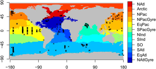
FIGURE 1. Biogeochemical provinces with station locations of sediment trap observations overlain. Locations are shown for profiles with more than two observations at a profile location at a particular time.

Statistical Modeling

We first describe the analysis and estimation of an individual profile which constitutes the base level of analysis. We then describe methods for aggregating profiles at the regional and global scale, starting with simple data aggregation at the biome level, then parameter aggregation of individually estimated profiles, then onto simultaneous estimation of a global hierarchical Bayesian model.

Model for a Single Organic Carbon Flux Profile

Individual profiles are modeled by a power-law curve known in oceanography as the Martin curve (Martin et al., 1987), which describes the steady state organic carbon flux attenuation with depth. The flux of organic carbon in moles per area per time at depth z takes the form

where $z_0$ is a reference depth taken as the base of the euphotic layer (where sufficient light is available for phytoplankton to perform photosynthesis and take up dissolved inorganic carbon). We approximate $z_0$ using satellite chlorophyll data (Lee et al., 2007). $F_0=F\left(z_0\right)$ is the flux at the reference depth and the exponent b controls the carbon flux attenuation with depth. This curve is obtained from the steady state solution of the following one-dimensional partial differential equation

where κ is the rate of organic carbon remineralization, $u\left(z\right)$ is the depth-dependence particle sinking rate with $u\left(z\right)=c_0+cz$ (Kriest and Oschlies, 2008). The attenuation coefficient in Eq. 1 is then defined as $b=\kappa /c$. In the ocean we expect the profile parameters b and $F_0$ to vary in time and space. We assume b will be non-positive because particulate organic carbon cannot be produced below the euphotic zone and will only attenuate with depth. This assumption implies constraints on the priors of the Bayesian analysis, explained below.

We estimate the parameters $F_0$ and b for a profile at a particular location given vertical measurements of $F\left(z\right)$. Taking the logarithm of Eq. 1 gives

where $a=\log \left(F_0\right)$. Equation 3 allows the estimation of a and b via simple linear regression, where b is the slope and a is the intercept.

Data Aggregation

Our first method of analysis directly aggregates the data to the group structure of interest. We aggregate the data into biomes and fit a single profile to the biome-level data. We report the fitted a and b parameters for each of the eight biomes and their associated uncertainties.

Parameter Aggregation

We perform a second analysis where we preserve profiles and fit individual a and b parameters to individually observed profiles. We perform a meta-analysis of the individual profiles by averaging the a and b parameters by biome post-hoc. We use inverse-variance weighted averaging, where parameters are averaged at the biome level according to the inverse of their respective uncertainties. The weighted averages take the form

where ${\overline{b}}_w\left(j\right)$ and ${\overline{a}}_w\left(j\right)$ are the average slope and intercept, respectively, for a particular biome j. In the above sums, the index i runs over the individual profiles within the jth biome, i.e. $b\left(i,j\right)$ and $a\left(i,j\right)$ are the individually estimated slopes and intercepts. We take $w_a\left(i,j\right)\propto {\sigma }_a^{-2}\left(i,j\right)$ and $w_b\left(i,j\right)\propto {\sigma }_b^{-2}\left(i,j\right)$, where ${\sigma }_a^2\left(i,j\right)$ and ${\sigma }_b^2\left(i,j\right)$ are the variances of the individually estimated parameters, with ${\displaystyle \sum _i{w}_a\left(i,j\right)}={\displaystyle \sum _i{w}_b\left(i,j\right)}=1$.

The biome-level weighted variances are

for the intercept and slope, respectively.

Bayesian Hierarchical Model

Our third approach involves fitting a single, global-scale hierarchical Bayesian model that captures variance due to biome, within-biome location, and timestamp in a single statistical framework. We follow Primeau (2006) who first proposed a hierarchical model for organic carbon flux observations based on a more limited dataset. In general, hierarchical Bayesian models can be represented as a directed acyclic graph (DAG) with successive conditional probabilities flowing from a priori assumptions on the base level of model parameters. The basic structure of the DAG for our model is shown in Figure 2.

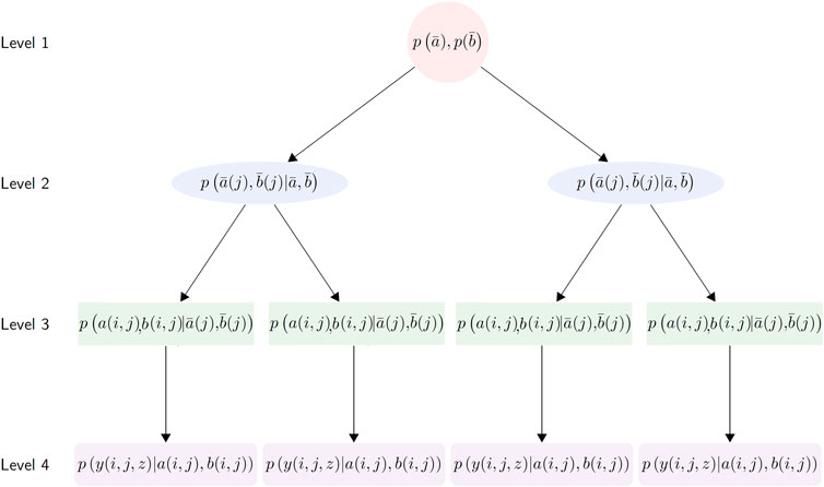
FIGURE 2. The directed acyclic graph (DAG) structure of the Bayesian hierarchical model. At level (1), the global-level parameters describe the mean profile across all biomes and stations. At level (2), the biome-level parameters are sampled conditional on the global level parameters in level (1). Level (3) samples parameters at the station-level of analysis from the biome-level distribution. Level (4) is the data-level of analysis, which constitutes the likelihood function of the observations, where the probability of the individual observations is evaluated conditional on the hierarchical network of parameters sampled previously.

At the top level of the model, we assume the mean global Martin curve profile is described by the parameters $\overline{a}$ and $\overline{b}$. For the particle flux to attenuate with increasing depth, we impose the constraint that all b parameters must be non-positive via truncated non-positive Gaussian probability distributions. At the biome-level of the model, the mean profile parameters differ from the global mean profile according to normal distributions, conditional on the global parameters. Specifically, the biome-specific mean parameters for biome j, denoted $\overline{a}\left(j\right)$ and $\overline{b}\left(j\right)$, have distributions

where the global variables $\overline{a}$ and $\overline{b}$ are used as inputs to the second level of the model. Parameters ϕ_a and ϕ_b are the variances of a and b, respectively. The truncated non-positive normal distribution is denoted with ${\mathcal{N}}^{\ast }$. The notation for conditional distributions given as $x|y$ is shorthand for $p\left(x|y\right)$.

For the station-level, we add an additional level to the model, conditional on the prior two. The station-level parameters, $a\left(i,j\right)$ and $b\left(i,j\right)$, have distributions

where ${\varphi }_a\left(j\right)$ and ${\varphi }_b\left(j\right)$ are the variances of the station-level parameters within a particular biome. We specify uniform priors for the biome and station-level parameter variances and estimate their posterior distribution from the data simultaneously with the as and bs. We tested for sensitivity to the uniform prior by also fitting a model where $p\left(\varphi \right)\propto {\varphi }^{-1}$, known as a Jeffrey’s prior, and found no appreciable statistical difference in the results under the two priors. This is consistent with the relatively large n of this study, in which case the data overwhelm differences in priors, provided the posterior is not close to an absolute bound. For smaller samples sizes, we note that hierarchical models can be sensitive to the choice of prior on the hierarchical variances (Gelman and Hill, 2006).

Finally, the data-level of the analysis assumes errors on individual flux measurements follow

where $y\left(i,j,z\right)$ is the log of the observed flux at station i in biome j at depth z, and ${\varphi }_y$ is the error variance of individual measurements. The conditional probabilities are written out semi-explicitly to demonstrate the sequential conditional probability distributions characteristic of hierarchical Bayesian models. The variance parameters were assumed implicitly in the description above. We note that the above model structure assumes that lower level probability distributions can be evaluated as conditionally independent, given values defined at upper levels, also referred to as exchangability. In the environmental realm, this assumption is rarely satisfied precisely due to inherent spatial and temporal correlations at many scales of environmental variability. However, our choice of biome definition follows from previous work demonstrating distinct ocean biogeochemical provinces (DeVries, 2014; Teng et al., 2014) where carbon flux processes follow more similar patterns within biomes than across biomes. Below we examine the model residuals across biomes to assess this assumption.

The hierarchical Bayesian model is fit via Markov Chain Monte Carlo (MCMC) sampling. MCMC repeatedly draws correlated random samples from the prior distribution of model parameters and runs them through the graph of conditional probabilities. MCMC sampling provides samples from the posterior distribution which characterizes the distribution of the model parameters after the data are taken into account. Sampling is required because no closed form solution is available for the hierarchical Bayesian regression with unknown variances and truncated normal distributions. We note that analytical forms for hierarchical model posteriors are available under particular statistical assumptions (Gelman and Hill, 2006); however, the MCMC approach applied here is fast and flexible and will yield robust inferences on a wider class of models. The high-level model interface provided by brms makes the model easy to implement and modify (Burkner, 2017). The brms implementation uses the general-purpose MCMC software package “Stan” to perform the sampling (Carpenter et al., 2017) which applies an advanced Hamiltonian Monte Carlo algorithm which has proven to be considerably faster than previously available MCMC software (Monnahan et al., 2016; Betancourt, 2017). The R, brms, and Stan code to fit the model is provided on GitHub (https://github.com/gregbritten/Britten_et_al_Frontiers_2019).

3 Results

Comparing data-aggregation to parameter-aggregation methods, we find that the data-aggregation method yields $\overline{a}\left(j\right)$ and $\overline{b}\left(j\right)$ parameters of larger magnitude and smaller uncertainty than parameter-aggregation across all biomes (Figure 3; Table 1). Averaging across biomes, the $\overline{a}\left(j\right)$ parameters estimated via data-aggregation were 15% more positive than those estimated via parameter aggregation, while the $\overline{b}\left(j\right)$ parameters were 39% more negative. Uncertainty intervals, on the other hand, were much larger in width for parameter aggregation. Uncertainty intervals for $\overline{a}\left(j\right)$via parameter aggregation were over 10 times wider than for data aggregation, while intervals for $\overline{b}\left(j\right)$ estimates were 7.5 times wider, on average.

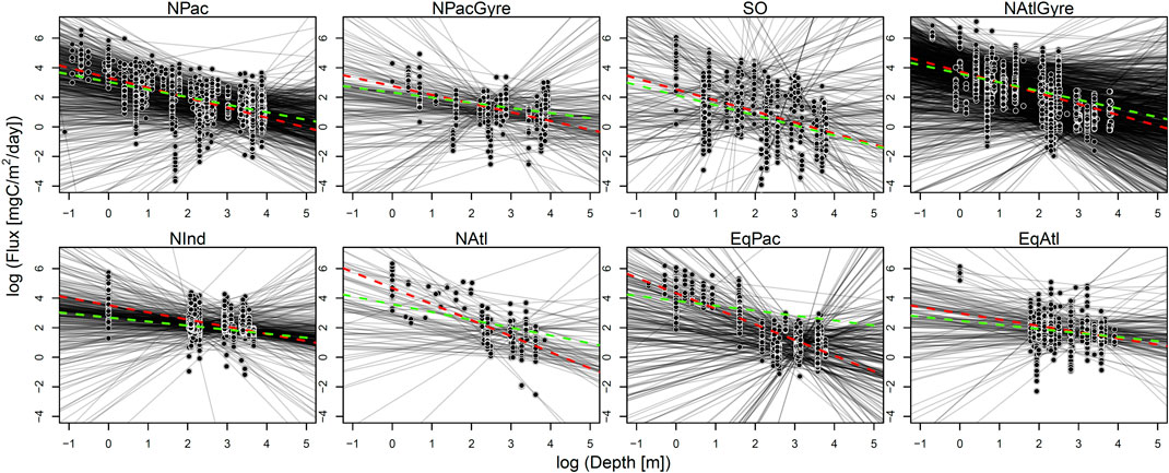
FIGURE 3. Results from data-aggregation and parameter-aggregation fits. For each biome, an individually fitted profile is shown in shaded black lines. The green dotted line is the parameter-aggregation fit (i.e., the uncertainty-weighted average of individual lines). The red dotted line is the fit for the data-aggregation method.

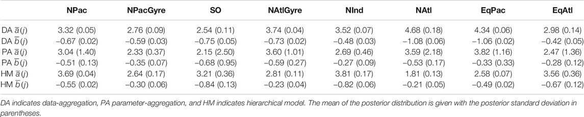
TABLE 1. Estimates for biome-level profile parameters across the three methods.

Uncertainty intervals for the hierarchical analysis were wider to that of the data-aggregation method, while both the hierarchical analysis and data-aggregation method both showed several-fold narrower uncertainty than parameter aggregation. The smaller uncertainty of the hierarchical and data aggregation methods reflects the greater power in using a larger number of observations to estimate parameters relative to parameter aggregation (Figure 4; Table 1). In contrast to parameter-aggregation and data-aggregation, we saw no consistent positive or negative directional difference in the hierarchical estimates relative to the others. For example, $\overline{a}\left(j\right)$ and $\overline{b}\left(j\right)$ parameters were both greater in magnitude for the Northern Indian Ocean (NInd) biome region using the hierarchical estimate, while $\overline{a}$ and $\overline{b}\left(j\right)$ were both smaller in magnitude for the North Atlantic (NAtl) using the hierarchical approach.

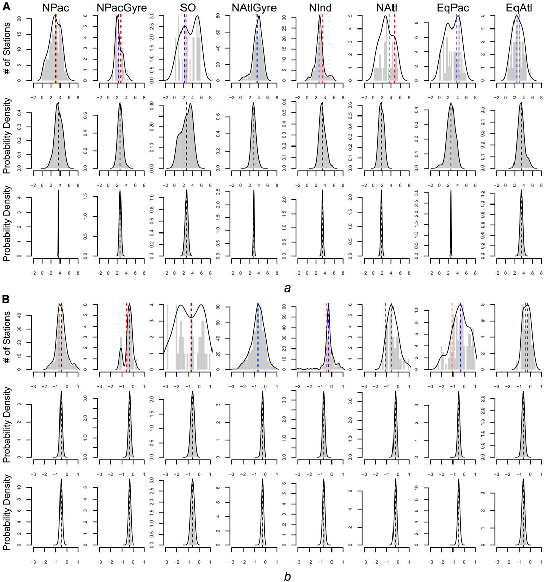
FIGURE 4. Estimates of a (panel set (A) and b (panel set (B) for all three methods. Top rows of a and b give the frequency distribution of parameters based on individual (non-hierarchical) estimates. Blue dashed line is the parameter-aggregation estimate for the biome-level mean (i.e., the uncertainty weighted average of the distribution). The red dashed line is the biome-level estimate via data aggregation. The middle rows give the distribution of station-level parameters for the hierarchical fit. Bottom rows give the distribution for the biome-level parameters for the hierarchical fit.

From a hypothesis-testing perspective, we evaluated the evidence for biome-level differences in profile parameters by comparing the overlap between posterior probability intervals for the biome-level a and b parameters (Table 1). Due to the large uncertainties yielded via parameter aggregation, we find only weak statistical evidence for biome-level differences for a and b. With the exception of NPacGyre and NInd, the 2σ uncertainty in a and b was on the order of 50%, or greater, relative to the mean, indicating that parameter aggregation can only detect the largest underlying biome-level differences. In contrast, uncertainty estimates for a and b via data aggregation and the hierarchical model were less than 15% of the mean, on average, indicating much stronger statistical separation. Importantly, however, hypothesis-tests (performed by evaluating the degree of overlap in the posterior probability distributions) from data aggregation vs. the hierarchical model result in different conclusions; for example, a test comparing $\overline{b}\left(j\right)$ for NInd vs. EqPac at the biome level would indicate strong statistical support for a larger $\overline{b}\left(j\right)$ in EqPac relative to NInd based on data aggregation, while the full hierarchical model supports the opposite, thus demonstrating the importance of treating group structure in estimating and interpreting model parameters.

Beyond the biome-level mean parameters, we find that the hierarchical model exhibits the expected shrinkage of parameter estimates where the variance of the station-level parameters within biomes, $a\left(i,j\right)$ and $b\left(i,j\right)$, are reduced in the hierarchical model (Figure 5). We quantify shrinkage by the reduction in variance seen in the station-level mean parameters fitted in the hierarchical context, relative to fitting individual profiles. We find that variance in station-level $a\left(i,j\right)$ parameters was reduced by between 73% and 95% across biomes with a mean of 87% when fitting the hierarchical model relative to fitting individually. Variance was reduced by more than 95% across all biomes for station-level $b\left(i,j\right)$ parameters.

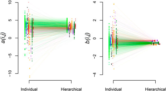
FIGURE 5. Shrinkage of station estimates toward the biome-level values. Results are shown for a (left panel) and b (right panel). Within panels, mean station-level parameter estimates are shown for the individual and hierarchical analysis. Biome groups have distinct colors and are horizontally offset relative to one another for visualization. Lines connect individual stations estimated with both approaches.

The effects of informative prior distributions are shown in Figure 6 where we compare our estimates of the distribution of $b\left(i,j\right)$ to fits without imposing a non-positive b. Without the constraint, all the posterior distributions contain a fraction of positive $b\left(i,j\right)$. This fraction was less than 1/1,000 for five out of eight biomes (NPac, SO, NInd, EqPac, and EqAtl). For the remaining NPacGyre, NAtlGyre, and NAtl biomes, the fraction was 3.7, 7.1, and 13.2%, respectively, indicating that the scientifically motivated prior distributions were required to constrain $b\left(i,j\right)$ into realistic non-positive values for these regions. This result reflects the importance of using scientifically informed prior distributions for constraining sampling noise in the observations.

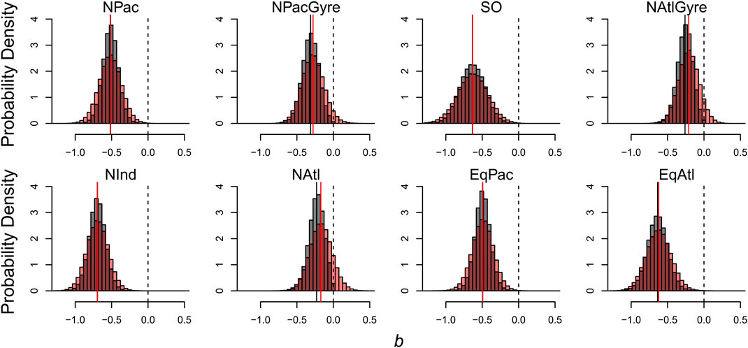
FIGURE 6. Effects of informative prior distributions on posterior model parameters. Shown are posterior distributions for b based on two forms of the model: gray histograms show posteriors for the model with the prior constraint that b is non-positive; red histograms show posteriors without the prior constraint.

Residuals of the data-aggregation and hierarchical model fit are shown in Figure 7. (Note that hierarchical model residuals are evaluated relative to the mean of the posterior predictions for individual observations.) In both models, the error distribution of individual observations within biomes are assumed to be independent draws from a Gaussian distribution. Residuals from data-aggregation method, however (Figure 7A), show obvious deviations from Gaussianity, with bimodal and skewed structure, while the hierarchical residual show more central symmetry, despite some evidence for heavier tails than would be expected from a normal distribution (e.g., the North Pacific). This poor residual structure for the data-aggregation method suggests the Gaussian assumptions are poorly met without taking into account the station-level variability within biomes. This is important since the data-aggregation showed lower uncertainty for several parameter estimates at the biome-level (Figure 4; Table 1), yet apparently did so via less appropriate statistical assumptions on the distribution of within-biome measurements. The hierarchical model explicitly captures this variability via explicit distributional assumptions on within-biome parameter variability, while simultaneously providing profile- and global-level inference.

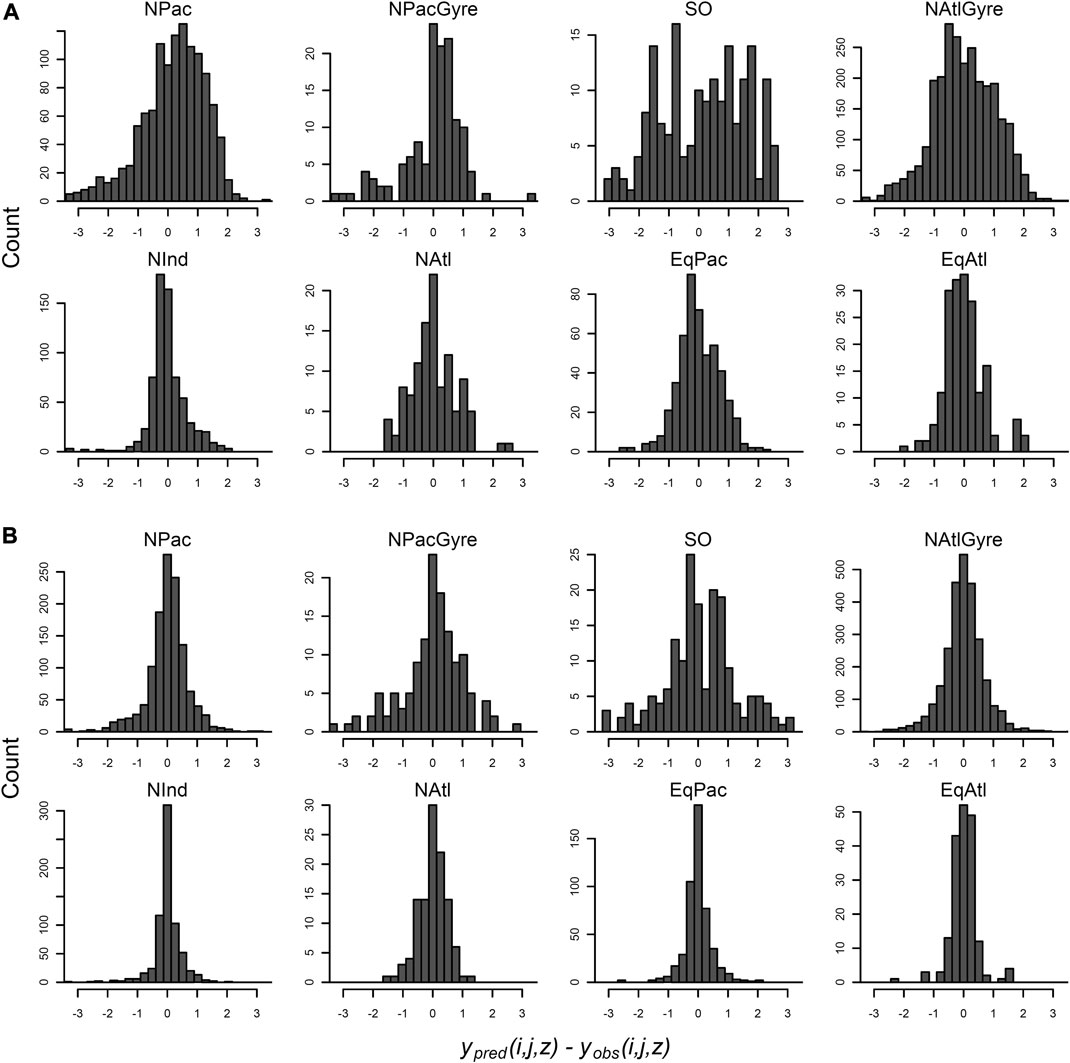
FIGURE 7. Distribution of data-level residuals for the data-aggregation method (A) and the hierarchical analysis (B). Residuals are evaluated at each latitude, longitude, depth combination, organized by biome-group. Residuals are for the hierarchical analysis are evaluated as the posterior mean prediction minus the observation.

4 Discussion

The growing public availability of environmental data compilations has highlighted the importance of modeling statistical heterogeneities that arise across environmental datasets for analytical or contextual reasons. Bayesian hierarchical modeling is well-suited for this purpose, however its benefits over simpler methods have been rarely quantified in applied settings. This study explicitly quantified these benefits point-by-point using a representative dataset, thus aiding researchers in their choice of the appropriate method for aggregated analysis of heterogeneous environmental data compilations.

The tendency for individual profiles to borrow information in the hierarchical model is determined by the distributional assumptions made about the parameters and their hierarchical structure. We adopted Gaussian assumptions for the parameter distributions and for the distributions of errors on the log-transformed organic flux observations. The former assumption is supported by an examination of the distribution of individual (non-hierarchical) estimates (Figure 4). The latter assumption is supported by our oceanographic understanding of marine biomes cited previously (Teng et al., 2014; Bisson et al., 2018; Cael et al., 2018), including previous statistical analysis of carbon flux observations (Bisson et al., 2018; Cael et al., 2018). The biome-level assumption is further supported by the examination of model residuals (Figure 7). However, more sophisticated hierarchical structures and distributions may also be appropriate for the data; for example, finer scale spatial aggregation may be appropriate, or alternative distributional assumptions on the slopes and intercepts. We note that both data-aggregation and the hierarchical analysis have the advantage of simultaneously using a greater number of observations in estimating the biome-level profiles. However, the data-aggregation method achieves low uncertainty via overly restrictive assumptions on the distribution of individual observations (Figure 7). The Bayesian hierarchical analysis achieves its level of confidence while appropriately treating group-level and within-group structure within the model hierarchy.

While hierarchical models can be fit via frequentist inference, the Bayesian approach allowed us to naturally incorporate chemically realistic non-positivity constraints on b via prior distributions on model parameters. The $b<0$ constraint was motivated by the expected attenuation of the flux with depth, as particulate organic carbon is continuously remineralized (and no longer produced) as it sinks toward the ocean floor. Implementing the constraint was straightforward in this framework where positive values are given zero prior probability at the appropriate levels in the hierarchy of parameters, which is propagated forward via Bayes’ theorem in the MCMC. This constraint reduced the posterior uncertainty in model parameters and excluded nonphysical values from the estimation. The simplicity contrasts with the frequentist approach to hierarchical model estimation (Zuur et al., 2009; Bates et al., 2013; Faraway, 2016; Pinheiro et al., 2019) where the $b<0$ constraint would be more challenging to implement and where distributional assumptions are highly constrained. Another benefit of Bayesian analysis is the direct interpretation of the posterior distributions as probabilities which can be propagated into subsequent calculations with the model parameters; for example in generating carbon flux predictions at a particular location. The increasing variety of advanced software technology makes Bayesian analysis increasingly attractive for use across the environmental sciences. Programmatically simple interfaces are easy to use, even for those with limited programming experience (Burkner, 2017; Carpenter et al., 2017).

It is important to note that some complexities in the data are not accounted for in this particular hierarchical model. A common bias in oceanography occurs via non-random sampling, where field campaigns target areas or events of specific interest, such as regions of high biological productivity (Briggs et al., 2011; Rembauville et al., 2015). This gives rise to systematic biases in observed carbon flux magnitude at the base of the euphotic zone; for example, due to the established positive correlation between primary productivity and sinking flux (Britten and Primeau, 2016). The model could be extended to capture this bias by introducing additional parameters; for example, with a model of the form $\log \left[F\left(z\right)\right]=a+b\log \left(\frac{z}{z_0}\right)+dP$, where P is the primary production estimated from satellite observations, that may help correct a bias on the intercept arising from over-sampling of highly productive regions. A more comprehensive model may also attempt to capture effects due to temperature (Marsay et al., 2015), seasonality (Briggs et al., 2011), mineral ballasting (Britten et al., 2017), among others. We encourage these extensions (work that is in progress by the authors), while reiterating that our purpose here was to assess the utility of the hierarchical Bayesian model for performing aggregated analysis, relative to simpler analytical approaches.

In terms of oceanographic results, we note differences in the biome-level parameters estimated here relative to those estimated via a biogeochemical inverse models (Teng et al., 2014). The largest relative differences appear to occur in low productivity areas; for eample in NAtlGyre and NPacGyre where we estimated $b=-0.23$ and $b=-0.30$, while (Teng et al., 2014) estimated $b=-0.64$ and $b=-0.51$, respectively. The cause of these differences is not clear and may be partly due to the biases mentioned above, issues related to hydrodynamic undersampling of sinking flux by sediment traps (Buesseler et al., 2007), or errors in the oceanographic inverse model. The oceanographic model in (Teng et al., 2014) resolves the mean annual carbon flux in each biome region, thus the biome aggregation allows a more direct comparison of flux parameters estimated from the model to those estimated from observations. Discrepancies between model-based and observational parameters at this scale provide the opportunity to better understand errors in the model or observations. Other spatial aggregations can be used to elucidate relationships at other spatial-temporal scales. A process-based study systematically comparing the biome-level parameters estimated via model-based and statistical methods is outside the scope of this paper, which would require testing additional statistical parameterizations of the model. We hope this paper helps pave the way for those efforts.

5 Conclusion

In summary, our case study has quantified the practical utility of hierarchical Bayesian analysis for performing aggregated analysis on environmental data compilations that contain statistical heterogeneities due to sample size, sampling methodology, time, space, and other potential sources of variation. These heterogeneities are common in environmental datasets and will be an increasing challenge as the publication of compiled datasets continues to increase in popularity. We argue that hierarchical Bayesian analysis is well-suited to handle these heterogeneities in accounting for group-level correlation while allowing the incorporation of a priori knowledge on the model parameters. Easy-to-use software tools are now readily available to implement hierarchical Bayesian analysis without expertise in computational statistics. We hope this case study provides a reference for environmental researchers faced with a choice of methods for analyzing heterogeneous compiled datasets.

Data Availability Statement

Publicly available datasets were analyzed in this study. This data can be found here: doi: 10.1594/PANGAEA.855600.

Author Contributions

GB, FP designed the research. GB, YM, LP, MA, CG, WW, BP, BC, FP contributed methods and/or data. GB, YM, LP, MA, CG, WW, BP, FP analyzed data and performed research. GB, YM, LP, MA, CG, WW, BP, BC, FP wrote the paper.

Funding

GB was supported by the Simons Collaboration on Computational Biogeochemical Modeling of Marine Ecosystems CBIOMES (Grant # 549931) and the Simons Foundation Postdoctoral Fellowship in Marine Microbial Ecology. BP was supported through funding from the United States Department of Energy grant DE-SC0016539 and the National Science Foundation grant 1658380.

Conflict of Interest

The authors declare that the research was conducted in the absence of any commercial or financial relationships that could be construed as a potential conflict of interest.

Acknowledgments

We acknowledge all the individual ocean scientists that contributed to the data that was compiled in Mouw et al. (2016), and to the authors of Mouw et al. (2016) who made this compilation available. We thank three reviewers who strengthened the manuscript and attendees of the Simons Foundation CBIOMES Annual Meeting who provided feedback on this paper.

References

Bates, D. M., Maechler, M., Bolker, B., and Walker, S. (2013). lme4: linear mixed-effects models using Eigen and S4. R package version 67. doi:10.18637/jss.v067.i01
Betancourt, M. (2017). A conceptual introduction to Hamiltonian Monte Carlo.Preprint: arXiv:170102424.
Bianchi, D., Dunne, J. P., Sarmiento, J. L., and Galbraith, E. D. (2012). Data-based estimates of suboxia, denitrification, and N2O production in the ocean and their sensitivities to dissolved O2. Glob. Biogeochem. Cycles 26, 1–13. doi:10.1029/2011gb004209
Bisson, K. M., Siegel, D. A., DeVries, T., Cael, B. B., and Buesseler, K. O. (2018). How data set characteristics influence ocean carbon export models. Glob. Biogeochem. Cycles 32, 1–17. doi:10.1029/2018gb005934
Blyth, C. R. (1972). On simpson’s paradox and the sure-thing principle. J. Am. Stat. Assoc. 67, 364–366. doi:10.1080/01621459.1972.10482387
Briggs, N., Perry, M. J., Cetinic, I., Lee, C., D’Asaro, E., Gray, A. M., et al. (2011). High resolution observations of aggregate flux during a sub polar North Atlantic spring bloom. Deep Sea Res. Part I: Oceanogr. Res. Pap. 58, 1031–1039. doi:10.1016/j.dsr.2011.07.007
Britten, G. L., and Primeau, F. W. (2016). Biome‐specific scaling of ocean productivity, temperature, and carbon export efficiency. Geophys. Res. Lett. 43, 5210–5216. doi:10.1002/2016gl068778
Britten, G. L., Wakamatsu, L., and Primeau, F. W. (2017). The temperature-ballast hypothesis explains carbon export efficiency observations in the Southern Ocean. Geophys. Res. Lett. 44, 1831–1838. doi:10.1002/2016gl072378
Brockwell, S. E., and Gordon, I. R. (2001). A comparison of statistical methods for meta-analysis. Stat. Med. 20, 825–840. doi:10.1002/sim.650 |
Buesseler, K. O. (1991). Do upper-ocean sediment traps provide an accurate record of particle flux?. Nature 353, 420–423. doi:10.1038/353420a0
Buesseler, K. O., Antia, A. N., Chen, M., Fowler, S. W., Gardner, W. D., Gustafsson, O., et al. (2007). An assessment of the use of sediment traps for estimating upper ocean particle fluxes. J Mar. Res. 65, 345–416. doi:10.1357/002224007781567621
Bürkner, P.-C. (2017). Brms: an R package for bayesian multilevel models using stan. J. Stat. Soft. 80. doi:10.18637/jss.v080.i01
Cael, B. B., Bisson, K., and Follett, C. L. (2018). Can rates of ocean primary production and biological carbon export Be related through their probability distributions?. Global Biogeochem Cycles 32, 954–970. doi:10.1029/2017GB005797
Carpenter, B., Gelman, A., Hoffman, M., Lee, D., Goodrich, B., Betancourt, M., et al. (2017). Journal of statistical software stan : a probabilistic programming language. J. Stat. Softw. 76, 1–32. doi:10.18637/jss.v076.i01
Clark, J. S. (2004). Why environmental scientists are becoming Bayesians. Ecol. Lett. 8, 2–14. doi:10.1111/j.1461-0248.2004.00702.x
Clark, J. S., and Gelfand, A. E. (2006). A future for models and data in environmental science. Trends Ecol. Evol. 21, 375–380. doi:10.1016/j.tree.2006.03.016 |
DeVries, T. (2014). The oceanic anthropogenic CO2sink: storage, air-sea fluxes, and transports over the industrial era. Glob. Biogeochem. Cycles 28, 631–647. doi:10.1002/2013GB004739
DeVries, T., and Primeau, F. (2011). Dynamically and observationally constrained estimates of water-mass distributions and ages in the global ocean. J. Phys. Oceanography 41, 2381–2401. doi:10.1175/jpo-d-10-05011.1
Draper, D. (1995). Inference and hierarchical modeling in the social sciences. J. Educ. Behav. Stat. 20, 115–147. doi:10.2307/1165353
Faraway, J. J. (2016). Extending the linear model with R. London, United Kingdom: Chapman and Hall/CRC.
Gelman, A., Carlin, J. B., Stern, H. S., Dunson, D. B., Vehtari, A., and Rubin, D. B. (2013). Bayesian data analysis. London, United Kingdom: Chapman and Hall/CRC.
Gelman, A., and Hill, J. (2006). Data analysis using regression and multilevel/hierarchical models. Cambridge, United Kingdom: Cambridge University Press.
Jonsen, I. D., Myers, R. A., and Flemming, J. M. (2003). Meta-analysis of animal movement using state-space models. Ecology 84, 3055–3063. doi:10.1890/02-0670
Kriest, I., and Oschlies, A. (2008). On the treatment of particulate organic matter sinking in large-scale models of marine biogeochemical cycles. Biogeosciences 5, 55–72. doi:10.5194/bg-5-55-2008
Lee, Z. P., Weidemann, A., Kindle, J., Arnone, R., Carder, K. L., and Davis, C. (2007). Euphotic zone depth: its derivation and implication to ocean-color remote sensing. J. Geophys. Res. Oceans 112. doi:10.1029/2006jc003802
Marsay, C. M., Sanders, R. J., Henson, S. A., Pabortsava, K., Achterberg, E. P., and Lampitt, R. S. (2015). Attenuation of sinking particulate organic carbon flux through the mesopelagic ocean. Proc. Natl. Acad. Sci. USA 112, 1089–1094. doi:10.1073/pnas.1415311112 |
Martin, J. H., Knauer, G. a., Karl, D. M., and Broenkow, W. W. (1987). VERTEX: carbon cycling in the northeast Pacific. Deep Sea Res. A, Oceanogr. Res. Pap. 34, 267–285. doi:10.1016/0198-0149(87)90086-0
Monnahan, C. C., Thorson, J. T., and Branch, T. A. (2016). Faster estimation of bayesian models in ecology using hamiltonian monte carlo. Methods Ecol. Evol. 1, 1–10. doi:10.1111/2041-210X.12681
Mouw, C. B., Barnett, A., Mckinley, G. A., Gloege, L., and Pilcher, D. (2016). Global ocean particulate organic carbon flux merged with satellite parameters. Earth Syst. Sci. Data 8, 531–541. doi:10.5194/essd-8-531-2016
Pearl, J. (2014). Comment: understanding simpson’s paradox. Am. Stat. 68, 8–13. doi:10.1080/00031305.2014.876829
Pinheiro, J., Bates, D., DebRoy, S., and Sarkar, D. (2019). nlme: linear and nonlinear mixed effects models. R. Package Version 3, 111.
Primeau, F. (2006). On the variability of the exponent in the power law depth dependence of POC flux estimated from sediment traps. Deep Sea Res. Oceanog. Res. Pap. 53, 1335–1343. doi:10.1016/j.dsr.2006.06.003
Primeau, F. W., Holzer, M., and DeVries, T. (2013). Southern Ocean nutrient trapping and the efficiency of the biological pump. J. Geophys. Res. Oceans 118, 2547–2564. doi:10.1002/jgrc.20181
Rembauville, M., Blain, S., Armand, L., Quéguiner, B., and Salter, I. (2015). Export fluxes in a naturally iron-fertilized area of the Southern Ocean - Part 2: importance of diatom resting spores and faecal pellets for export. Biogeosciences 12, 3171–3195. doi:10.5194/bg-12-3171-2015
Sereno, M. (2016). A Bayesian approach to linear regression in astronomy. Mon. Not. R. Astron. Soc. 455, 2149–2162. doi:10.1093/mnras/stv2374
Sharkey, P., and Winter, H. (2019). A Bayesian spatial hierarchical model for extreme precipitation in Great Britain. Environmetrics 30. doi:10.1002/env.2529
Sharma, S. (2017). Markov chain Monte Carlo methods for Bayesian data analysis in astronomy. Annu. Rev. Astron. Astrophys. 55, 213–259. doi:10.1146/annurev-astro-082214-122339
Sivia, D., and Skilling, J. (2006). Data analysis: a bayesian tutorial. Oxford, United Kingdom: Oxford University Press.
Teng, Y.-C., Primeau, F. W., Moore, J. K., Lomas, M. W., and Martiny, A. C. (2014). Global-scale variations of the ratios of carbon to phosphorus in exported marine organic matter. Nat. Geosci. 7, 895–898. doi:10.1038/ngeo2303
Thorson, J. T., Cope, J. M., Kleisner, K. M., Samhouri, J. F., Shelton, A. O., and Ward, E. J. (2015). Giants’ shoulders 15 years later: lessons, challenges and guidelines in fisheries meta-analysis. Fish Fish. 16, 342–361. doi:10.1111/faf.12061
Keywords: data compilation, hierarchical model, bayesian, meta-analysis, shrinkage, prior
Citation: Britten GL, Mohajerani Y, Primeau L, Aydin M, Garcia C, Wang W-L, Pasquier B, Cael BB and Primeau FW (2021) Evaluating the Benefits of Bayesian Hierarchical Methods for Analyzing Heterogeneous Environmental Datasets: A Case Study of Marine Organic Carbon Fluxes. Front. Environ. Sci. 9:491636. doi: 10.3389/fenvs.2021.491636
Received: 14 August 2019; Accepted: 22 January 2021;
Published: 09 March 2021.
Edited by:
Juergen Pilz, University of Klagenfurt, AustriaReviewed by:
Gunter Spöck, University of Klagenfurt, AustriaTianhai Cheng, Institute of Remote Sensing and Digital Earth, China
Gregor Laaha, University of Natural Resources and Life Sciences Vienna, Austria
Copyright © 2021 Britten, Mohajerani, Primeau, Aydin, Garcia, Wang, Pasquier, Cael and Primeau. This is an open-access article distributed under the terms of the Creative Commons Attribution License (CC BY). The use, distribution or reproduction in other forums is permitted, provided the original author(s) and the copyright owner(s) are credited and that the original publication in this journal is cited, in accordance with accepted academic practice. No use, distribution or reproduction is permitted which does not comply with these terms.
*Correspondence: Gregory L. Britten, gbritten@mit.edu