Prey fear of a specialist predator in a tri-trophic food web can eliminate the superpredator

Fakhry, Nabaa Hassain; Naji, Raid Kamel; Smith?, Stacey R.; Haque, Mainul

doi:10.3389/fams.2022.963991

ORIGINAL RESEARCH article

Front. Appl. Math. Stat., 03 November 2022
Sec. Mathematical Biology
Volume 8 - 2022 | https://doi.org/10.3389/fams.2022.963991

Prey fear of a specialist predator in a tri-trophic food web can eliminate the superpredator

Nabaa Hassain Fakhry¹

Raid Kamel Naji¹

Stacey R. Smith?²

Mainul Haque³^*

¹Department of Mathematics, College of Science, University of Baghdad, Baghdad, Iraq
²Department of Mathematics and Faculty of Medicine, The University of Ottawa, Ottawa, ON, Canada
³School of Mathematical Science, The University of Nottingham Ningbo China, Ningbo, China

We propose an intraguild predation ecological system consisting of a tri-trophic food web with a fear response for the basal prey and a Lotka–Volterra functional response for predation by both a specialist predator (intraguild prey) and a generalist predator (intraguild predator), which we call the superpredator. We prove the positivity, existence, uniqueness, and boundedness of solutions, determine all equilibrium points, prove global stability, determine local bifurcations, and illustrate our results with numerical simulations. An unexpected outcome of the prey's fear of its specialist predator is the potential eradication of the superpredator.

Introduction

A functioning ecosystem depends on the framework of food webs that it supports [1]. Food webs involve many types of predator–prey interactions, which are fundamental interactions for sustaining species [2]. Interaction between the prey and the predator can be affected by factors such as refuge, disease, stage structure, competition, and fear [3–7]. Intraguild predation (IGP), on the other hand, is described as predator–prey interactions among consumers who may be fighting for limited resources. In natural communities, there is a growing body of literature emphasizing the relevance of intraguild predation [8, 9]. Three species are involved in the simplest intraguild predation model: a superpredator (IG predator), a specialist predator (IG prey), and a basal prey. Bai et al. recently suggested a three-species IGP food web model with the IG predator, IG prey, and basal prey, in which the basal prey grows logistically with a large Allee effect [10]. They looked into the model's local and global dynamics, focusing on the impact of the Allee effect and discovered that the intraguild predation food web model has rich and complicated dynamic behavior and that a large Allee effect in the basal prey raises the danger of extinction for not only the basal prey but also the IG prey or/and IG predator.

Many predators in food webs are superpredators, who may not restrict their diets to a specific prey species but feed also on other predators [11]. Therefore, superpredators are expected to compete not only with other predators for food and space but in many cases also through intraguild predation [5, 12, 13]. Predators induce indirect effects such as fear in prey that can change the prey's behavior [14]. Fear takes the form of sustained psychological stress on the prey, as prey species are always wary of possible attack [15]. Suraci et al. experimentally showed that fear of large carnivores reduces mesocarnivore foraging, which benefits the mesocarnivore's prey [16].

A handful of mathematical models have studied the effect of fear on food webs. Panday et al. investigated the impact of fear in a tri-trophic food chain model, with prey fear in response to both predators [15], from the middle predator to the generalist predator [17] and with delays [18]. Cong et al. introduced a fear-adjusted birth rate to a three-species food web [19]. Hossain et al. limited the growth of the prey due to fear in an intraguild predation model [20]. Mukerjee incorporated interspecific competition and fear affecting the death rate of the prey [21]. Ibrahim et al. limited prey growth due to fear of the generalist predator and showed that fear could have a stabilizing effect on the system [22]. Mondal et al. showed that the prey's fear of predators was responsible for the increase in intraspecific competition among the prey species [23]. Roy et al. showed that fear could play a destablizing role if it caused a reduction in the birth rate of susceptible prey, whereas the levels of fear responsible for the increase in the intraspecies competition of susceptible prey and eradication of the disease prevalence could stabilize an otherwise unstable system [24]. Maity et al. considered time-varying fear effects, showing that periodic solutions could arise [25]. Hossain et al. showed that perceived fear of predators could reduce the prey birth rate [26]. Tiwari et al. showed that seasonal variations in the level of prey fear generated higher-order periodic solutions [27].

Here, we examine the impact of fear on the dynamical behavior of an IGP food web system in which the prey responds with fear to the specialist predator but not the superpredator; because the superpredator has alternative food sources, it will be less dangerous to the basal prey compared to the IG prey. To the best of our knowledge, this is the first model to examine this effect.

Food-web model formulation

Our food web consists of a prey at the first level, a specialist predator at the second level, and a superpredator at the third level. Let x(t), y(t), and z(t) be the population densities at time t for the prey, specialist predator, and superpredator, respectively. The prey grows logistically in the absence of predators, while it has a fear property of predation in the presence of the specialist predator. Hence, the intrinsic growth rate of prey becomes $\frac{r}{1 + k y}$ , which is a monotonic decreasing function of both k and y, where k represents the fear rate [28]. The food transport attack rates are given by the parameters a₁, a₂, and a₃, with conversion rates e₁, e₂, and e₃. Finally, the predators face natural death rates d₁ and d₂ for the specialist predator and superpredator, respectively. The dynamics of the food web with fear can be represented mathematically by the following set of differential equations:

\begin{array}{l} \begin{array}{l} \frac{d x}{d t} = r x (1 - x) (\frac{1}{1 + k y}) - a_{1} x y - a_{2} x z = x f_{1} (x, y, z), \\ \frac{d y}{d t} = e_{1} a_{1} x y - a_{3} y z - d_{1} y = y f_{2} (x, y, z), \\ \frac{d z}{d t} = e_{2} a_{2} x z + e_{3} a_{3} y z - d_{2} z = z f_{3} (x, y, z) . \end{array} & (1) \end{array}

Initial conditions satisfy x(t) ≥ 0, y(t) ≥ 0, and z(t) ≥ 0, and all parameters are assumed to be positive.

The interaction functions f_i (i = 1, 2, 3) are continuous and have continuous partial derivatives and are thus Lipschitzian, so system (1) has a unique solution. Furthermore, for any initial condition in $ℝ_{+}^{3}$ , the solution of system (1) is positive and uniformly bounded as shown in the following theorem. Hence, system (1) will be a dissipative system.

Theorem (1): The domain of system (1), $ℝ_{+}^{3}$ , is positively invariant, and all solutions of system (1) starting in $ℝ_{+}^{3}$ are uniformly bounded.

Proof. Let x(t), y(t), and z(t) be any solution of system (1). Since the solution (x(t), y(t), z(t)) of the system (1) with initial condition in $ℝ_{+}^{3}$ exists and is unique on [0 , δ), where 0 < δ ≤ +∞, we have:

\begin{array}{l} x (t) = x (0) e^{\int_{0}^{t} [r (1 - x (s)) (\frac{1}{1 + k y (s)}) - a_{1} y (s) - a_{2} z (s)] d s} \geq 0 \end{array}

\begin{array}{l} y (t) = y (0) e^{\int_{0}^{t} [e_{1} a_{1} x (s) - a_{3} z (s) - d_{1}] d s} \geq 0 \end{array}

\begin{array}{l} z (t) = z (0) e^{\int_{0}^{t} [e_{2} a_{2} x (s) + e_{3} a_{3} y (s) - d_{2}] d s} \geq 0 . \end{array}

From the first equation of system (1):

\begin{array}{l} \frac{d x}{d t} \leq r x (1 - x) . \end{array}

Then, it is easy to verify that $x (t) \leq \frac{r}{4}$ for all t.

Let = x + y + z. Then, since e_i ∈ (0, 1); i = 1, 2, 3, we have

$\frac{d W}{d t} \leq \frac{r}{4} - M [x + y + z]$ ,

where M = min{1, d₁, d₂}. Solving the following linear differential inequality

\begin{array}{l} \frac{d W}{d t} + M W \leq \frac{r}{4}, \end{array}

we obtain that, as t → ∞,

\begin{array}{l} W (t) \leq \frac{r}{4 M} . \end{array}

Existence of equilibrium points

System (1) has at most five nonnegative biologically feasible equilibrium points. The trivial equilibrium E₀ = (0, 0, 0) always exists. The axial equilibrium E₁ = (1, 0, 0) always exists on the boundary of the first octant. The specialist-free equilibrium point, $E_{2} = (\bar{x}, 0, \bar{z})$ , where

\begin{array}{l} \bar{x} = \frac{d_{2}}{e_{2} a_{2}} and \bar{z} = \frac{r (1 - \bar{x})}{a_{2}}, & (2a) \end{array}

exists provided that

\begin{array}{l} d_{2} < e_{2} a_{2} . & (2b) \end{array}

The superpredator-free equilibrium point, $E_{3} = (\hat{x}, \hat{y}, 0)$ , where

\begin{array}{l} \hat{x} = \frac{d_{1}}{e_{1} a_{1}} and \hat{y} = - \frac{1}{2 k} + \frac{1}{2 a_{1} k} \sqrt{a_{1}^{2} + 4 k r \frac{(e_{1} a_{1} - d_{1})}{e_{1}}}, & (3a) \end{array}

exists, provided that

\begin{array}{l} d_{1} < e_{1} a_{1} . & (3b) \end{array}

There is also an interior equilibrium point, $E_{4} = (x^{*}, y^{*}, z^{*})$ , where

\begin{array}{l} y^{^{*}} = \frac{d_{2} - e_{2} a_{2} x^{^{*}}}{e_{3} a_{3}} and z^{^{*}} = \frac{e_{1} a_{1} x^{^{*}} - d_{1}}{a_{3}}, & (4a) \end{array}

with x^* a positive root of the following second-order polynomial equation:

\begin{array}{l} β_{1} x^{2} + β_{2} x + β_{3} = 0, & (4b) \end{array}

where

\begin{array}{l} β_{1} = e_{2} a_{1} {a_{2}}^{2} k [e_{1} e_{3} - e_{2}], \end{array}

\begin{array}{l} \begin{matrix} β_{2} = e_{2} e_{3} a_{1} a_{2} a_{3} - r {e_{3}}^{2} {a_{3}}^{2} + 2 e_{2} a_{1} a_{2} k d_{2} - e_{1} e_{3} a_{1} a_{2} {a_{3}}^{2} \\ - e_{1} e_{3} a_{1} a_{2} k d_{2} - e_{2} e_{3} {a_{2}}^{2} k d_{1}, \end{matrix} \end{array}

\begin{array}{l} β_{3} = r {e_{3}}^{2} {a_{3}}^{2} - e_{3} a_{1} a_{3} d_{2} - a_{1} k {d_{2}}^{2} + e_{3} a_{2} {a_{3}}^{2} d_{1} + e_{3} a_{2} k d_{1} d_{2} . \end{array}

Therefore, there is a unique interior equilibrium point in the interior of $ℝ_{+}^{3}$ provided that the following conditions hold:

\begin{array}{l} \frac{d_{1}}{e_{1} a_{1}} < x^{^{*}} < \frac{d_{2}}{e_{2} a_{2}} & (4c) \end{array}

\begin{array}{l} \begin{matrix} β_{1} > 0; β_{3} < 0 \\ O R \\ β_{1} < 0; β_{3} > 0 \end{matrix}} . & (4d) \end{array}

Persistence

Next, we determine the requirements that ensure persistence in the system (1). Because the types of attractors available in the boundary planes affect the creation of our IGP food web model's persistence conditions, an analysis of the dynamics in the boundary planes of the IGP food web system is conducted. System (1) has two subsystems: the first occurs in the absence of the superpredator (IG predator) and the second occurs in the absence of the specialist predator (IG prey). The first subsystem is

\begin{array}{l} \begin{array}{l} \frac{d x}{d t} = x [\frac{r (1 - x)}{1 + k y} - a_{1} y] = x f_{1} (x, y) \\ \frac{d y}{d t} = y [e_{1} a_{1} x - d_{1}] = y g_{1} (x, y) . \end{array} & (5) \end{array}

The second subsystem can be written as follows:

\begin{array}{l} \begin{array}{l} \frac{d x}{d t} = x [r (1 - x) - a_{2} z] = x f_{2} (x, z) \\ \frac{d z}{d t} = z [e_{2} a_{2} x - d_{2}] = z g_{2} (x, z) . \end{array} & (6) \end{array}

Subsystem (5) has a unique positive equilibrium point in the interior of xy-plane given by $(\hat{x}, \hat{y}) \equiv E_{3}$ , while subsystem (6) has a unique positive equilibrium point in the interior of xz-plane given by $(\bar{x}, \bar{z}) \equiv E_{2}$ . The interior equilibrium point of subsystem (5) corresponds to system (1)'s superpredator-free equilibrium point; similarly, the interior equilibrium point of subsystem (6) corresponds to system (1)'s specialist-predator-free equilibrium point. The dynamics around these equilibrium points can be described in the following theorem.

Theorem (2): There are no periodic dynamics in the interior of xy-plane or the xz-plane.

Proof. Define a continuously differential function $B (x, y) = \frac{1}{x y}$ . Then, we have:

\begin{array}{l} Δ = \frac{\partial (B f_{1})}{\partial x} + \frac{\partial (B g_{1})}{\partial y} = - \frac{r}{y (1 + k y)} . \end{array}

Clearly, Δ has the same sign and does not equal zero almost everywhere in a simply connected region of the xy-plane. By the Dulac–Bendixson criterion, system (1) has no periodic solutions lying entirely in the interior of xy−plane. The second part follows by using the Dulac function $C (x, z) = \frac{1}{x z}$ .

Theorem (3): System (1) is uniformly persistent in the interior of $ℝ_{+}^{3},$ provided that

\begin{array}{l} e_{1} a_{1} > d_{1}, & (7a) \end{array}

\begin{array}{l} e_{2} a_{2} > d_{2}, & (7b) \end{array}

\begin{array}{l} e_{1} a_{1} \bar{x} > a_{3} \bar{z} + d_{1}, & (7c) \end{array}

\begin{array}{l} e_{2} a_{2} \hat{x} + e_{3} a_{3} \hat{y} > d_{2} . & (7d) \end{array}

Proof. Consider the function $(x, y, z) = x^{b_{1}} y^{b_{2}} z^{b_{3}}$ , where b_i, i = 1, 2, 3, are positive constants and U(x, y, z) is a C¹ nonnegative function in the interior of $ℝ_{+}^{3}$ . Hence, we have

$\frac{d U}{d t} = \frac{\partial U}{\partial x} \frac{d x}{d t} + \frac{\partial U}{\partial y} \frac{d y}{d t} + \frac{\partial U}{\partial z} \frac{d z}{d t}$ ,

with

\begin{array}{l} \frac{\partial U}{\partial x} = b_{1} x^{(b_{1} - 1)} y^{b_{2}} z^{b_{3}}, \end{array}

\begin{array}{l} \frac{\partial U}{\partial y} = b_{2} x^{b_{1}} y^{(b_{2} - 1)} z^{b_{3}}, \end{array}

\begin{array}{l} \frac{\partial U}{\partial z} = b_{3} x^{b_{1}} y^{b_{2}} z^{(b_{3} - 1)} . \end{array}

Therefore,

\begin{array}{l} \begin{array}{l} Ψ (x, y, z) = \frac{(\frac{d U}{d t})}{U (x, y, z)} = \frac{b_{1}}{x} \frac{d x}{d t} + \frac{b_{2}}{y} \frac{d y}{d t} + \frac{b_{3}}{z} \frac{d z}{d t}, \\ = b_{1} [r (1 - x) (\frac{1}{1 + k y}) - a_{1} y - a_{2} z] \\ + b_{2} [e_{1} a_{1} x - a_{3} z - d_{1}] + b_{3} [e_{2} a_{2} x + e_{3} a_{3} y - d_{2}] . \end{array} \end{array}

Since there are no periodic solutions in the boundary planes of the system (1), it follows that system (1) is uniformly persistent provided that Ψ(E_i) > 0 for each i = 1, 2, 3. We have

\begin{array}{l} Ψ (E_{1}) = b_{2} [e_{1} a_{1} - d_{1}] + b_{3} [e_{2} a_{2} - d_{2}], \end{array}

\begin{array}{l} Ψ (E_{2}) = b_{2} [e_{1} a_{1} \bar{x} - a_{3} \bar{z} - d_{1}], \end{array}

\begin{array}{l} Ψ (E_{3}) = b_{3} [e_{2} a_{2} \hat{x} + e_{3} a_{3} \hat{y} - d_{2}] . \end{array}

Consequently, conditions (7a)–(7d) satisfy Ψ(E_i) > 0 for each i = 1, 2, 3.

Global stability analysis

Here, we use Lyapunov functions to investigate the global stability of equilibria.

Theorem (4): The axial equilibrium point E₁ = (1, 0, 0) is globally asymptotically stable provided that the following sufficient condition holds:

\begin{array}{l} e_{2} < e_{1} e_{3} < \frac{d_{2}}{a_{2}} . & (8) \end{array}

Proof. Consider the following positive-definite, real-valued function around E₁:

\begin{array}{l} V_{1} = c_{1} [x - 1 - ln x] + c_{2} y + c_{3} z . \end{array}

Then, we have:

\begin{array}{l} \begin{array}{l} \frac{d V_{1}}{d t} = - \frac{c_{1} r}{1 + k y} {(x - 1)}^{2} - (c_{1} - c_{2} e_{1}) a_{1} x y - (c_{1} - c_{3} e_{2}) a_{2} x z \\ - (c_{2} - c_{3} e_{3}) a_{3} y z - (c_{2} d_{1} - c_{1} a_{1}) y - (c_{3} d_{2} - c_{1} a_{2}) z . \end{array} \end{array}

Then, by choosing c₁ = e₁, c₂ = 1 and $c_{3} = \frac{1}{e_{3}}$ , we obtain

\begin{array}{l} \frac{d V_{1}}{d t} = - \frac{e_{1} r}{1 + k y} {(x - 1)}^{2} - (e_{1} - \frac{e_{2}}{e_{3}}) a_{2} x z - (d_{1} - e_{1} a_{1}) y \\ - (\frac{d_{2}}{e_{3}} - e_{1} a_{2}) z . \end{array}

Clearly, under condition (8), $\frac{d V_{1}}{d t}$ is negative definite. Moreover, since V₁ is radially unbounded, the axial equilibrium point E₁ = (1, 0, 0) is globally asymptotically stable.

Theorem (5): The specialist-free equilibrium point $E_{2} = (\bar{x}, 0, \bar{z})$ is globally asymptotically stable provided that the following sufficient conditions hold:

\begin{array}{l} a_{1} \bar{x} < \frac{d_{1}}{e_{1}} + \frac{e_{3} a_{3}}{e_{2}} \bar{z}, & (9a) \end{array}

\begin{array}{l} e_{1} e_{3} < e_{2} . & (9b) \end{array}

Proof. Consider the following positive-definite, real-valued function around E₂:

\begin{array}{l} V_{2} = c_{1} [x - \bar{x} - \bar{x} ln \frac{x}{\bar{x}}] + c_{2} y + c_{3} [z - \bar{z} - \bar{z} ln \frac{z}{\bar{z}}] . \end{array}

Then, we have:

\begin{array}{l} \begin{array}{l} \frac{d V_{2}}{d t} = - c_{1} r {(x - \bar{x})}^{2} - a_{2} [c_{1} - c_{3} e_{2}] (x - \bar{x}) (z - \bar{z}) \\ - (c_{1} - c_{2} e_{1}) a_{1} x y \\ - (c_{2} d_{1} - c_{1} a_{1} \bar{x} + c_{3} e_{3} a_{3} \bar{z}) y - (c_{2} - c_{3} e_{3}) a_{3} y z . \end{array} \end{array}

Then, by choosing c₁ = 1, $c_{2} = \frac{1}{e_{1}}$ and $c_{3} = \frac{1}{e_{2}}$ , we have:

\begin{array}{l} \frac{d V_{2}}{d t} = - r {(x - \bar{x})}^{2} - (\frac{d_{1}}{e_{1}} + \frac{e_{3} a_{3}}{e_{2}} \bar{z} - a_{1} \bar{x}) y \\ - (\frac{1}{e_{1}} - \frac{e_{3}}{e_{2}}) a_{3} y z . \end{array}

Obviously, under conditions (9a)–(9b), $\frac{d V_{2}}{d t}$ is negative definite. Moreover, since V₂ is radially unbounded, the specialist-free equilibrium point $E_{2} = (\bar{x}, 0, \bar{z})$ is globally asymptotically stable.

Theorem (6): The superpredator-free equilibrium point $E_{3} = (\hat{x}, \hat{y}, 0)$ is globally asymptotically stable, provided that, in addition to condition (9b), the following sufficient conditions hold:

\begin{array}{l} a_{2} \hat{x} + \frac{a_{3}}{e_{1}} \hat{y} < \frac{d_{2}}{e_{2}}, & (10a) \end{array}

\begin{array}{l} (x - \hat{x}) (y - \hat{y}) > 0 . & (10b) \end{array}

Proof. Consider the following positive-definite, real-valued function around E₃:

\begin{array}{l} V_{3} = c_{1} [x - \hat{x} - \hat{x} ln \frac{x}{\hat{x}}] + c_{2} [y - \hat{y} - \hat{y} ln \frac{y}{\hat{y}}] + c_{3} z . \end{array}

Then, we have

\begin{array}{l} \begin{array}{l} \frac{d V_{3}}{d t} = - \frac{c_{1} r {(x - \hat{x})}^{2}}{R} - \frac{c_{1} r k (1 - \hat{x}) (x - \hat{x}) (y - \hat{y})}{R \hat{R}} \\ - (c_{1} - c_{2} e_{1}) a_{1} (x - \hat{x}) (y - \hat{y}) - (c_{1} - c_{3} e_{2}) a_{2} x z \\ - (c_{2} - c_{3} e_{3}) a_{3} y z - (c_{3} d_{2} - c_{1} a_{2} \hat{x} - c_{2} a_{3} \hat{y}) z, \end{array} \end{array}

where R = (1 + ky) and $\hat{R} = (1 + k \hat{y})$ . Then, by choosing c₁ = 1, $c_{2} = \frac{1}{e_{1}}$ and $c_{3} = \frac{1}{e_{2}}$ , we obtain:

\begin{array}{l} \frac{d V_{3}}{d t} \leq - \frac{r {(x - \hat{x})}^{2}}{R} - \frac{r k (1 - \hat{x}) (x - \hat{x}) (y - \hat{y})}{R \hat{R}} \\ - (\frac{1}{e_{1}} - \frac{e_{3}}{e_{2}}) a_{3} y z - (\frac{d_{2}}{e_{2}} - a_{2} \hat{x} - \frac{a_{3}}{e_{1}} \hat{y}) z . \end{array}

Under conditions (10a)–(10b), $\frac{d V_{3}}{d t}$ is negative definite. Since V₃ is radially unbounded, the superpredator-free equilibrium point $E_{3} = (\hat{x}, \hat{y}, 0)$ is globally asymptotically stable.

Theorem (7): The coexistence equilibrium point $E_{4} = (x^{*}, y^{*}, z^{*})$ is globally asymptotically stable provided that, in addition to condition (9b), the following sufficient condition holds:

\begin{array}{l} (x - x^{^{*}}) (y - y^{^{*}}) > 0 . & (11) \end{array}

Proof. Consider the following positive-definite, real-valued function around E₄:

\begin{array}{l} V_{4} = c_{1} [x - x^{^{*}} - x^{^{*}} ln \frac{x}{x^{^{*}}}] + c_{2} [y - y^{^{*}} - y^{^{*}} ln \frac{y}{y^{^{*}}}] \\ + c_{3} [z - z^{^{*}} - z^{^{*}} ln \frac{z}{z^{^{*}}}] . \end{array}

Then, we have:

\begin{array}{l} \begin{array}{l} \frac{d V_{4}}{d t} = - \frac{c_{1} r {(x - x^{^{*}})}^{2}}{R} - \frac{c_{1} r k (1 - x^{^{*}}) (x - x^{^{*}}) (y - y^{^{*}})}{R R^{^{*}}} \\ \begin{matrix} - (c_{1} - c_{2} e_{1}) a_{1} (x - x^{^{*}}) (y - y^{^{*}}) \\ - (c_{2} - c_{3} e_{3}) a_{3} (y - y^{^{*}}) (z - z^{^{*}}) \\ - (c_{1} - c_{3} e_{2}) a_{2} (x - x^{^{*}}) (z - z^{^{*}}), \end{matrix} \end{array} \end{array}

where R^* = 1 + ky^*. Then, by choosing c₁ = e₂, c₂ = e₃, and c₃ = 1, we have

\begin{array}{l} \frac{d V_{4}}{d t} = - \frac{e_{2} r {(x - x^{^{*}})}^{2}}{R} - \frac{e_{2} r k (1 - x^{^{*}}) (x - x^{^{*}}) (y - y^{^{*}})}{R R^{^{*}}} \\ - (e_{2} - e_{1} e_{3}) a_{1} (x - x^{^{*}}) (y - y^{^{*}}) . \end{array}

Then, under condition (11) with (9b), $\frac{d V_{4}}{d t}$ is negative definite. Since V₄ is radially unbounded, the coexistence equilibrium point $E_{4} (x^{*}, y^{*}, z^{*})$ is globally asymptotically stable.

Bifurcation analysis

In this section, we investigate the effect of varying parameter values on the dynamics of the system (1) using local bifurcation analysis and the Sotomayor theorem [29]. First, we rewrite system (1) in the vector form as follows:

\begin{array}{l} \frac{d X}{d t} = F (X), X = {(x, y, z)}^{T} and F = {(x f_{1}, y f_{2}, z f_{3})}^{T} . \end{array}

The second derivative of F with respect to X can be written as:

\begin{array}{l} D^{2} F (U, U) = \\ (\begin{matrix} - \frac{2 r {u_{1}}^{2}}{1 + k y} - \frac{2 k r (1 - 2 x) u_{1} u_{2}}{{(1 + k y)}^{2}} - 2 a_{1} u_{1} u_{2} - 2 a_{2} u_{1} u_{3} + \frac{2 k^{2} r x (1 - x) {u_{2}}^{2}}{{(1 + k y)}^{3}} \\ 2 e_{1} a_{1} u_{1} u_{2} - 2 a_{3} u_{2} u_{3} \\ 2 e_{2} a_{2} u_{1} u_{3} + 2 e_{3} a_{3} u_{2} u_{3} \end{matrix}), & (12) \end{array}

where $U = {(u_{1}, u_{2}, u_{3})}^{T}$ is a general vector.

Theorem (8): Assume that $d_{2} = e_{2} a_{2} (\equiv {d_{2}}^{*})$ . Then system (1) undergoes a transcritical bifurcation at the axial equilibrium point E₁, but neither a saddle node nor a pitchfork bifurcation can occur if

\begin{array}{l} e_{1} a_{1} < d_{1} . & (13) \end{array}

Proof. The Jacobian matrix of system (1) at the axial equilibrium point E₁ with $d_{2} = e_{2} a_{2} (\equiv {d_{2}}^{*})$ can be written as:

\begin{array}{l} J_{1} = J (E_{1}, {d_{2}}^{*}) = [\begin{matrix} - r - a_{1} - a_{2} \\ 0 e_{1} a_{1} - d_{1} 0 \\ 0 0 0 \end{matrix}] . \end{array}

J₁ has eigenvalues ${λ_{11}}^{*} = - r < 0$ , ${λ_{12}}^{*} = e_{1} a_{1} - d_{1} < 0$ under condition (13), and ${λ_{13}}^{*} = 0$ . Hence, the necessary but not sufficient condition for a bifurcation is satisfied, and E₁ is a non-hyperbolic point.

Let $Φ_{1} = {(v_{11}, v_{12}, v_{13})}^{T}$ be the eigenvector of J₁ corresponding to the eigenvalue ${λ_{13}}^{*} = 0$ . Straightforward computation gives $Φ_{1} = {(β_{1} v_{13}, 0, v_{13})}^{T}$ , where v₁₃ represents any nonzero real number and $β_{1} = - \frac{a_{2}}{r} < 0$ .

Let $Ψ_{1} = {(ψ_{11}, ψ_{12}, ψ_{13})}^{T}$ be the eigenvector of ${J_{1}}^{T}$ corresponding to the eigenvalue ${λ_{13}}^{*} = 0$ . Direct calculation shows that $Ψ_{1} = {(0, 0, ψ_{13})}^{T}$ , where ψ₁₃ is any nonzero real number. Because $\frac{\partial F}{\partial d_{2}} = F_{d_{2}} = {(0, 0, - z)}^{T}$ , we obtain that $F_{d_{2}} (E_{1}, {d_{2}}^{*}) = {(0, 0, 0)}^{T}$ , which yields:

\begin{array}{l} {Ψ_{1}}^{T} [F_{d_{2}} (E_{1}, {d_{2}}^{^{*}})] = 0 . \end{array}

By Sotomayor's theorem, system (1) at E₁ with $d_{2} = {d_{2}}^{*}$ does not experience a saddle-node bifurcation. Moreover, we have

\begin{array}{l} {Ψ_{1}}^{T} [D F_{d_{2}} (E_{1}, {d_{2}}^{^{*}}) Φ_{1}] = - v_{13} Ψ_{13} \neq 0, \end{array}

where DF_d₂ represents the derivative of F_d₂ with respect to X. Applying equation (12) at $(E_{1}, {d_{2}}^{*})$ with the eigenvector Φ₁, we obtain that

\begin{array}{l} {Ψ_{1}}^{T} [D^{2} F (E_{1}, {d_{2}}^{^{*}}) (Φ_{1}, Φ_{1})] = 2 e_{2} a_{2} β_{1} {v_{13}}^{2} ψ_{13} \neq 0 . \end{array}

By Sotomayor's theorem, system (1) near the equilibrium point E₁ with $d_{2} = {d_{2}}^{*}$ undergoes a transcritical bifurcation, but a pitchfork bifurcation cannot occur.

Theorem (9): System (1) at the specialist-free equilibrium point E₂ undergoes a transcritical bifurcation when $d_{1} = e_{1} a_{1} \bar{x} + a_{3} \bar{z} (\equiv {d_{1}}^{*})$ , but neither a saddle-node nor a pitchfork bifurcation can occur, provided

\begin{array}{l} {e_{1} e_{3} a_{1} a}_{2} + r e_{3} a_{3} \neq e_{2} a_{2} [k r (1 - \bar{x}) + a_{1}] . & (14) \end{array}

Proof. The Jacobian matrix of system (1) at the specialist-free equilibrium point E₂ with $d_{1} = {d_{1}}^{*}$ takes the form:

\begin{array}{l} J_{2} = J (E_{2}, {d_{1}}^{^{*}}) = [\begin{matrix} - r \bar{x} & - k r \bar{x} (1 - \bar{x}) - a_{1} \bar{x} & - a_{2} \bar{x} \\ 0 & 0 & 0 \\ e_{2} a_{2} \bar{z} & e_{3} a_{3} \bar{z} & 0 \end{matrix}] . \end{array}

J₂ has eigenvalues

\begin{array}{l} {λ_{21}}^{^{*}} = - \frac{r \bar{x}}{2} + \frac{1}{2} \sqrt{{(r \bar{x})}^{2} - 4 e_{2} {a_{2}}^{2} \bar{x} \bar{z}}, \\ {λ_{23}}^{^{*}} = - \frac{r \bar{x}}{2} - \frac{1}{2} \sqrt{{(r \bar{x})}^{2} - 4 e_{2} {a_{2}}^{2} \bar{x} \bar{z}}, \end{array}

while ${λ_{22}}^{*} = 0$ ; hence, the necessary but not sufficient condition for a bifurcation is satisfied, and E₂ is a non-hyperbolic point.

Let $Φ_{2} = {(v_{21}, v_{22}, v_{23})}^{T}$ be the eigenvector of J₂ corresponding to the zero eigenvalue. Straightforward computation gives $Φ_{2} = {(α_{1} v_{22}, v_{22}, α_{2} v_{22})}^{T}$ , where v₂₂ represents any nonzero real number, with

\begin{array}{l} α_{1} = - \frac{e_{3} a_{3}}{e_{2} a_{2}} and α_{2} = \frac{r e_{3} a_{3} - [k r (1 - \bar{x}) + a_{1}] e_{2} a_{2}}{e_{2} {a_{2}}^{2}} . \end{array}

Let $Ψ_{2} = {(ψ_{21}, ψ_{22}, ψ_{23})}^{T}$ be the eigenvector of ${J_{2}}^{T}$ corresponding to the zero eigenvalue. Direct calculation shows that $Ψ_{2} = {(0, ψ_{22}, 0)}^{T}$ , where ψ₂₂ is any nonzero real number. Because $\frac{\partial F}{\partial d_{1}} = F_{d_{1}} = {(0, - y, 0)}^{T}$ , we obtain that $F_{d_{1}} (E_{2}, {d_{1}}^{*}) = {(0, 0, 0)}^{T}$ , which yields

\begin{array}{l} {Ψ_{2}}^{T} [F_{d_{1}} (E_{2}, {d_{1}}^{^{*}})] = 0 . \end{array}

Thus, by Sotomayor's theorem, system (1) at E₂ with $d_{1} = {d_{1}}^{*}$ does not experience a saddle-node bifurcation. Moreover, we have:

\begin{array}{l} {Ψ_{2}}^{T} [D F_{d_{1}} (E_{2}, {d_{1}}^{^{*}}) Φ_{2}] = - v_{22} ψ_{22} \neq 0, \end{array}

where DF_d₁ represents the derivative of F_d₁ with respect to X. Using equation (12) at $(E_{2}, {d_{1}}^{*})$ with the eigenvector Φ₂, we obtain that

\begin{array}{l} {Ψ_{2}}^{T} [D^{2} F (E_{2}, {d_{1}}^{^{*}}) (Φ_{2}, Φ_{2})] = (2 e_{1} a_{1} α_{1} - 2 a_{3} α_{2}) {v_{22}}^{2} ψ_{22} . \end{array}

It is easy to verify that ${Ψ_{2}}^{T} [D^{2} F (E_{2}, {d_{1}}^{*}) (Φ_{2}, Φ_{2})] \neq 0$ due to condition (14). Hence, by Sotomayor's theorem, system (1) near the equilibrium point E₂ with $d_{1} = {d_{1}}^{*}$ undergoes a transcritical bifurcation but a pitchfork bifurcation cannot occur.

Theorem (10): At the superpredator-free equilibrium point E₃, system (1) undergoes a transcritical bifurcation when $d_{2} = e_{2} a_{2} \hat{x} + e_{3} a_{3} \hat{y} (\equiv {d_{2}}^{*})$ , but neither a saddle-node nor a pitchfork bifurcation can occur, provided

\begin{array}{l} e_{2} a_{2} [k r (1 - \hat{x}) + a_{1} {(1 + k \hat{y})}^{2}] \neq \\ e_{3} (1 + k \hat{y}) [a_{3} r + e_{1} a_{1} a_{2} (1 + k \hat{y})] . & (15) \end{array}

Proof. The Jacobian matrix of system (1) at the superpredator-free equilibrium point E₃ with $d_{2} = {d_{2}}^{*}$ is

\begin{array}{l} J_{3} = J (E_{3}, {d_{2}}^{^{*}}) = [\begin{matrix} - \frac{r \hat{x}}{1 + k \hat{y}} & - \frac{k r \hat{x} (1 - \hat{x})}{{(1 + k \hat{y})}^{2}} - a_{1} \hat{x} & - a_{2} \hat{x} \\ e_{1} a_{1} \hat{y} & 0 & - a_{3} \hat{y} \\ 0 & 0 & 0 \end{matrix}] . \end{array}

J₃ has eigenvalues

\begin{array}{l} {λ_{31}}^{^{*}} = - \frac{r \hat{x}}{2 (1 + k \hat{y})} \\ + \frac{1}{2} \sqrt{{(\frac{r \hat{x}}{1 + k \hat{y}})}^{2} - 4 e_{1} a_{1} \hat{y} (\frac{k r \hat{x} (1 - \hat{x})}{{(1 + k \hat{y})}^{2}} + a_{1} \hat{x})}, \end{array}

\begin{array}{l} {λ_{32}}^{^{*}} = - \frac{r \hat{x}}{2 (1 + k \hat{y})} \\ - \frac{1}{2} \sqrt{{(\frac{r \hat{x}}{1 + k \hat{y}})}^{2} - 4 e_{1} a_{1} \hat{y} (\frac{k r \hat{x} (1 - \hat{x})}{{(1 + k \hat{y})}^{2}} + a_{1} \hat{x})}, \end{array}

while ${λ_{33}}^{*} = 0$ ; hence, the necessary but not sufficient condition for bifurcation is satisfied, and E₃ is a non-hyperbolic point.

Let $Φ_{3} = {(v_{31}, v_{32}, v_{33})}^{T}$ be the eigenvector of J₃ corresponding to the zero eigenvalue. Straightforward computation gives $Φ_{3} = {(s_{1} v_{33}, s_{2} v_{33}, v_{33})}^{T}$ , where v₃₃ represents any nonzero real number, while

\begin{array}{l} s_{1} = \frac{a_{3}}{e_{1} a_{1}} and s_{2} = - [\frac{r a_{3} (1 + k \hat{y}) + e_{1} a_{1} a_{2} {(1 + k \hat{y})}^{2}}{e_{1} a_{1} [k r (1 - \hat{x}) + a_{1} {(1 + k \hat{y})}^{2}]}] . \end{array}

Let $Ψ_{3} = {(ψ_{31}, ψ_{32}, ψ_{33})}^{T}$ be the eigenvector of ${J_{3}}^{T}$ corresponding to the zero eigenvalue. Direct calculation shows that $Ψ_{3} = {(0, 0, ψ_{33})}^{T}$ , where ψ₃₃ is any nonzero real number. Because $\frac{\partial F}{\partial d_{2}} = F_{d_{2}} = {(0, 0, - z)}^{T}$ , we obtain $F_{d_{2}} (E_{3}, {d_{2}}^{*}) = {(0, 0, 0)}^{T}$ , which yields

\begin{array}{l} {Ψ_{3}}^{T} [F_{d_{2}} (E_{3}, {d_{2}}^{^{*}})] = 0 . \end{array}

Thus, by Sotomayor's theorem, system (1) at E₃ with $d_{2} = {d_{2}}^{*}$ does not experience a saddle-node bifurcation. Moreover, we have:

\begin{array}{l} {Ψ_{3}}^{T} [D F_{d_{2}} (E_{3}, d_{2}) Φ_{3}] = - v_{33} ψ_{33} \neq 0, \end{array}

where DF_d₂ represents the derivative of F_d₂ with respect to X. By using equation (12) at $(E_{3}, {d_{2}}^{*})$ with the eigenvector Φ₃, we obtain that:

\begin{array}{l} {Ψ_{3}}^{T} [D^{2} F (E_{3}, {d_{2}}^{^{*}}) (Φ_{3}, Φ_{3})] = (2 e_{2} a_{2} s_{1} + 2 e_{3} a_{3} s_{2}) {v_{33}}^{2} ψ_{33} . \end{array}

Straightforward computation shows that ${Ψ_{3}}^{T} [D^{2} F (E_{3}, {d_{2}}^{*}) (Φ_{3}, Φ_{3})] \neq 0$ due to condition (15). Thus, by Sotomayor's theorem, system (1) near the equilibrium point E₃ with $d_{2} = {d_{2}}^{*}$ undergoes a transcritical bifurcation, but a pitchfork bifurcation cannot occur.

Theorem (11): System (1) undergoes a saddle-node bifurcation at the coexistence equilibrium point E₄, but neither a transcritical nor a pitchfork bifurcation can occur when e₃ passes through the value ${e_{3}}^{*} = \frac{b_{12} b_{23} b_{31}}{(b_{11} b_{23} - b_{13} b_{21}) a_{3} z^{*}}$ , provided the following conditions hold:

\begin{array}{l} (\frac{k r x^{^{*}} (1 - x^{^{*}})}{{(1 + k y^{^{*}})}^{2}} + a_{1} x^{^{*}}) e_{2} a_{2} > (\frac{r x^{^{*}}}{1 + k y^{^{*}}}) {e_{3}}^{^{*}} a_{3}, & (16a) \end{array}

\begin{array}{l} \frac{a_{1} a_{2}}{a_{3}} (\frac{e_{2}}{{e_{3}}^{^{*}}} - e_{1}) - \frac{r}{(1 + k y^{^{*}})} \times \\ [1 - \frac{k (1 - 2 x^{^{*}}) e_{2} a_{2}}{(1 + k y^{^{*}}) {e_{3}}^{^{*}} a_{3}} - \frac{k^{2} x^{^{*}} (1 - x^{^{*}}) {(e_{1} a_{1})}^{2}}{{(1 + k y^{^{*}})}^{2} {a_{3}}^{2}}] \neq 0 . & (16b) \end{array}

Proof. Direct computation shows that system (1) at the coexistence equilibrium point and ${e_{3} = e_{3}}^{*}$ has Jacobian matrix

\begin{array}{r} J_{4} = J (E_{4}, {e_{3}}^{*}) = [\begin{matrix} - \frac{r x^{^{*}}}{1 + k y^{*}} & - \frac{k r x^{*} (1 - x^{*})}{{(1 + k y^{*})}^{2}} - a_{1} x^{*} & - a_{2} x^{*} \\ e_{1} a_{1} y^{*} & 0 & - a_{3} y^{*} \\ e_{2} a_{2} z^{*} & {e_{3}}^{*} a_{3} z^{*} & 0 \end{matrix}] \\ = {[b_{i j}]}_{3 \times 3} . \end{array}

Straightforward computation shows that |J₄| = 0, under condition (16a). Hence, J₄ has two eigenvalues with negative real parts, and the third one is λ^* = 0. It follows that E₄ becomes a non-hyperbolic equilibrium point.

Let $Φ_{4} = {(v_{41}, v_{42}, v_{43})}^{T}$ be the eigenvector of J₄ corresponding to the eigenvalue λ^* = 0. Straightforward computation gives $Φ_{4} = {(v_{41}, δ_{1} v_{41}, δ_{2} v_{41})}^{T}$ , where v₄₁ represents any nonzero real number, $δ_{1} = - \frac{b_{31}}{{b_{32}}^{*}} < 0$ and $δ_{2} = - \frac{b_{21}}{b_{23}} > 0$ .

Let $Ψ_{4} = {(ψ_{41}, ψ_{42}, ψ_{43})}^{T}$ be the eigenvector of ${J_{4}}^{T}$ corresponding to the eigenvalue λ^* = 0. Direct calculation shows that $Ψ_{4} = {(ψ_{41}, μ_{1} ψ_{41}, μ_{2} ψ_{41})}^{T}$ , where ψ₃₃ is any nonzero real number, with $μ_{1} = - \frac{b_{13}}{b_{23}} < 0$ and $μ_{2} = - \frac{b_{12}}{b_{32}} > 0$ .

Since $\frac{\partial F}{\partial e_{3}} = F_{e_{3}} = {(0, 0, a_{3} y z)}^{T}$ , we have $F_{e_{3}} (E_{4}, {e_{3}}^{*}) = {(0, 0, a_{3} y^{*} z^{*})}^{T}$ , which yields

\begin{array}{l} {Ψ_{4}}^{T} [F_{e_{3}} (E_{4}, {e_{3}}^{^{*}})] = a_{3} μ_{2} y^{^{*}} z^{^{*}} ψ_{41} \neq 0 . \end{array}

By Sotomayor's theorem, transcritical and pitchfork bifurcations cannot occur while the first condition of the saddle-node bifurcation is satisfied. Moreover, from equation (12) with $E_{4}, {e_{3}}^{*}$ and Φ₄, we obtain that:

\begin{array}{l} \begin{matrix} D^{2} F (E_{4}, {e_{3}}^{^{*}}) (Φ_{4}, Φ_{4}) = {2 v_{41}}^{2} \times \\ (\begin{matrix} - \frac{r}{1 + k y^{^{*}}} - \frac{k r (1 - 2 x^{^{*}}) δ_{1}}{{(1 + k y^{^{*}})}^{2}} - a_{1} δ_{1} - a_{2} δ_{2} + \frac{k^{2} r x^{^{*}} (1 - x^{^{*}}) {δ_{2}}^{2}}{{(1 + k y^{^{*}})}^{3}} \\ e_{1} a_{1} δ_{1} - a_{3} δ_{1} δ_{2} \\ e_{2} a_{2} δ_{2} + {e_{3}}^{^{*}} a_{3} δ_{1} δ_{2} \end{matrix}) . \end{matrix} \end{array}

Hence,

\begin{array}{l} \begin{matrix} Ψ_{4}^{T} [D^{2} F (E_{4}, {e_{3}}^{^{*}}) (Φ_{4}, Φ_{4})] = {2 v_{41}}^{2} ψ_{41} \times \\ [- \frac{r}{1 + k y^{^{*}}} - \frac{k r (1 - 2 x^{^{*}}) δ_{1}}{{(1 + k y^{^{*}})}^{2}} - a_{1} δ_{1} - a_{2} δ_{2} \\ + \frac{k^{2} r x^{^{*}} (1 - x^{^{*}}) {δ_{2}}^{2}}{{(1 + k y^{^{*}})}^{3}} + e_{1} a_{1} δ_{1} μ_{1} - a_{3} δ_{1} δ_{2} μ_{1} + e_{2} a_{2} δ_{2} μ_{2} \\ + {e_{3}}^{^{*}} a_{3} δ_{1} δ_{2} μ_{2}] . \end{matrix} \end{array}

Further computation shows that

\begin{array}{l} \begin{array}{l} {Ψ_{4}}^{T} [D^{2} F (E_{4}, {e_{3}}^{^{*}}) (Φ_{4}, Φ_{4})] = {2 v_{41}}^{2} ψ_{41} [\frac{a_{1} a_{2}}{a_{3}} (\frac{e_{2}}{{e_{3}}^{^{*}}} - e_{1}) \\ - \frac{r}{(1 + k y^{^{*}})} [1 - \frac{k (1 - 2 x^{^{*}}) e_{2} a_{2}}{(1 + k y^{^{*}}) {e_{3}}^{^{*}} a_{3}} - \frac{k^{2} x^{^{*}} (1 - x^{^{*}}) {(e_{1} a_{1})}^{2}}{{(1 + k y^{^{*}})}^{2} {a_{3}}^{2}}]] . \end{array} \end{array}

Using condition (16b), we have ${Ψ_{4}}^{T} [D^{2} F (E_{4}, {e_{3}}^{*}) (Φ_{4}, Φ_{4})] \neq 0$ . Hence, system (1) has a saddle-node bifurcation at E₄ when $e_{3} = {e_{3}}^{*}$ .

Theorem (12): System (2) undergoes a Hopf bifurcation around E₄ when $e_{3} = {e_{3}}^{* *}$ , if and only if the following conditions hold:

\begin{array}{l} (\frac{k r x^{*} (1 - x^{*})}{{(1 + k y^{*})}^{2}} + a_{1} x^{*}) e_{2} a_{2} < (\frac{r x^{*}}{1 + k y^{*}}) e_{3} a_{3}, & (17a) \end{array}

\begin{array}{l} {[A ({e_{3}}^{^{* *}}) B ({e_{3}}^{^{* *}})]}^{^{'}} < C^{^{'}} ({e_{3}}^{^{* *}}), & (17b) \end{array}

where

\begin{array}{l} A = - b_{11} > 0, \end{array}

\begin{array}{l} B = - b_{12} b_{21} - b_{13} b_{31} - b_{23} b_{32}^{*} > 0, \end{array}

\begin{array}{l} C = b_{23} (b_{11} b_{32}^{*} - b_{12} b_{31}) - b_{13} b_{21} b_{32}^{*}, \end{array}

with $b_{32}^{*} = {e_{3}}^{* *} a_{3} z^{*}$ and,

\begin{array}{r} {e_{3}}^{* *} = \frac{1}{e_{1} a_{1} a_{2} a_{3} y^{^{*}} z^{*}} [[\frac{k r (1 - x^{*})}{{(1 + k y^{*})}^{2}} - a_{1}] \times \\ (e_{1} a_{1} y^{*} (\frac{r x^{*}}{1 + k y^{*}}) + e_{2} a_{2} a_{3} y^{*} z^{*}) + e_{2} {a_{2}}^{2} z^{*} (\frac{r x^{*}}{1 + k y^{*}})] . \end{array}

Proof. Consider the Jacobian matrix J₄ given in Theorem (11), where $e_{3} = {e_{3}}^{* *}$ . It is simple to determine that the characteristic equation is

\begin{array}{l} λ^{3} + A λ^{2} + B λ + C = 0 . & (18) \end{array}

Obviously, condition (17a) guarantees that C > 0. A straightforward computation shows that AB = C when $e_{3} = {e_{3}}^{* *}$ . Hence, the characteristic equation (18) becomes

\begin{array}{l} (λ^{2} + B) (λ + A) = 0 . & (19) \end{array}

Consequently, we obtain that λ₁ = −A and $λ_{2, 3} = \pm i \sqrt{B} = \pm i δ_{2} ({e_{3}}^{* *})$ . Therefore, the Jacobian matrix has one negative real eigenvalue and two pure imaginary complex conjugates when $e_{3} = {e_{3}}^{* *}$ . As a result, the first criterion for having a Hopf bifurcation is met.

Moreover, where e₃ belongs to the neighborhood of ${e_{3}}^{* *}$ , the eigenvalues become λ_2,3 = δ₁(e₃) ± iδ₂(e₃).

Next, we substitute δ₁(e₃) + iδ₂(e₃) into equation (18) and take the derivative of the resulting equation with respect to e₃. Equating their real and imaginary parts, we obtain that

\begin{array}{l} \begin{array}{l} H_{1} (e_{3}) δ_{1}^{^{'}} (e_{3}) - H_{2} (e_{3}) δ_{2}^{^{'}} (e_{3}) = - H_{3} (e_{3}), \\ H_{2} (e_{3}) δ_{1}^{^{'}} (e_{3}) + H_{1} (e_{3}) δ_{2}^{^{'}} (e_{3}) = - H_{4} (e_{3}), \end{array} & (20) \end{array}

where

\begin{array}{l} H_{1} (e_{3}) = 3 {[δ_{1} (e_{3})]}^{2} + 2 A (e_{3}) δ_{1} (e_{3}) - 3 {[δ_{2} (e_{3})]}^{2} + B (e_{3}) . \end{array}

\begin{array}{l} H_{2} (e_{3}) = 6 δ_{1} (e_{3}) δ_{2} (e_{3}) + 2 A (e_{3}) δ_{2} (e_{3}) . \end{array}

\begin{array}{r} H_{3} (e_{3}) = A^{^{'}} {(e_{3}) [δ_{1} (e_{3})]}^{2} - A^{^{'}} {(e_{3}) [δ_{2} (e_{3})]}^{2} + B^{^{'}} (e_{3}) δ_{1} (e_{3}) \\ + C^{^{'}} (e_{3}) . \end{array}

\begin{array}{l} H_{4} (e_{3}) = 2 A^{^{'}} (e_{3}) {δ_{1} (e_{3}) δ}_{2} (e_{3}) + B^{^{'}} (e_{3}) δ_{2} (e_{3}) . \end{array}

Solving system (20) for $δ_{1}^{^{'}} (e_{3})$ gives

\begin{array}{l} δ_{1}^{^{'}} (e_{3}) = - \frac{H_{1} (e_{3}) H_{3} (e_{3}) + H_{2} (e_{3}) H_{4} (e_{3})}{{[H_{2} (e_{3})]}^{2} + {(e_{3}) [H_{2} (e_{3})]}^{2}} . \end{array}

The result follows if and only if $δ_{1}^{^{'}} (e_{3}) \neq 0$ or, equivalently, H₁(e₃)H₃(e₃) + H₂(e₃)H₄(e₃) ≠ 0 when $e_{3} = {e_{3}}^{* *}$ . Note that we have the following:

\begin{array}{l} δ_{1} ({e_{3}}^{^{* *}}) = 0 and δ_{2} ({e_{3}}^{^{* *}}) = \sqrt{B ({e_{3}}^{^{* *}})} . \end{array}

\begin{array}{l} H_{1} ({e_{3}}^{^{* *}}) = - 2 B ({e_{3}}^{^{* *}}) . \end{array}

\begin{array}{l} H_{2} ({e_{3}}^{^{* *}}) = 2 A ({e_{3}}^{^{* *}}) \sqrt{B ({e_{3}}^{^{* *}})} . \end{array}

\begin{array}{l} H_{3} ({e_{3}}^{^{* *}}) = - A^{^{'}} ({e_{3}}^{^{* *}}) [B ({e_{3}}^{^{* *}})] + C^{^{'}} ({e_{3}}^{^{* *}}) . \end{array}

\begin{array}{l} H_{4} ({e_{3}}^{^{* *}}) = B^{^{'}} ({e_{3}}^{^{* *}}) \sqrt{B ({e_{3}}^{^{* *}})} . \end{array}

Consequently,

\begin{array}{l} \begin{array}{l} H_{1} ({e_{3}}^{^{* *}}) H_{3} ({e_{3}}^{^{* *}}) + H_{2} ({e_{3}}^{^{* *}}) H_{4} ({e_{3}}^{^{* *}}) \\ = 2 A^{^{'}} ({e_{3}}^{^{* *}}) B^{2} ({e_{3}}^{^{* *}}) - 2 B ({e_{3}}^{^{* *}}) \\ C^{^{'}} ({e_{3}}^{^{* *}}) + 2 A ({e_{3}}^{^{* *}}) B^{^{'}} ({e_{3}}^{^{* *}}) B ({e_{3}}^{^{* *}}) \\ = - 2 B ({e_{3}}^{^{* *}}) [C^{^{'}} ({e_{3}}^{^{* *}}) - (A^{^{'}} ({e_{3}}^{^{* *}}) \\ B ({e_{3}}^{^{* *}}) + A ({e_{3}}^{^{* *}}) B^{^{'}} ({e_{3}}^{^{* *}})] . \end{array} \end{array}

Condition (17b) ensures that $H_{1} ({e_{3}}^{* *}) H_{3} ({e_{3}}^{* *}) + H_{2} ({e_{3}}^{* *}) H_{4} ({e_{3}}^{* *}) \neq 0$ .

Hence, the system has a Hopf bifurcation because $δ_{1}^{^{'}} (e_{3}) > 0$ under the conditions (17a)–(17b).

Numerical simulations

To illustrate the global dynamics of the system and confirm our analytical findings, we numerically simulated a hypothetical set of parameter values. Consider the following set of parameters:

\begin{array}{l} \begin{array}{l} r = 1, k = 1, a_{1} = 1, a_{2} = 0.5, a_{3} = 0.75, e_{1} = 0.75 \\ e_{2} = 0.25, e_{3} = 0.25, d_{1} = 0.05, d_{2} = 0.1 . \end{array} & (21) \end{array}

Using these data, system (1) asymptotically approaches the coexistence equilibrium point E₄ = (0.5, 0.2, 0.43), as shown in Figure 1.

FIGURE 1

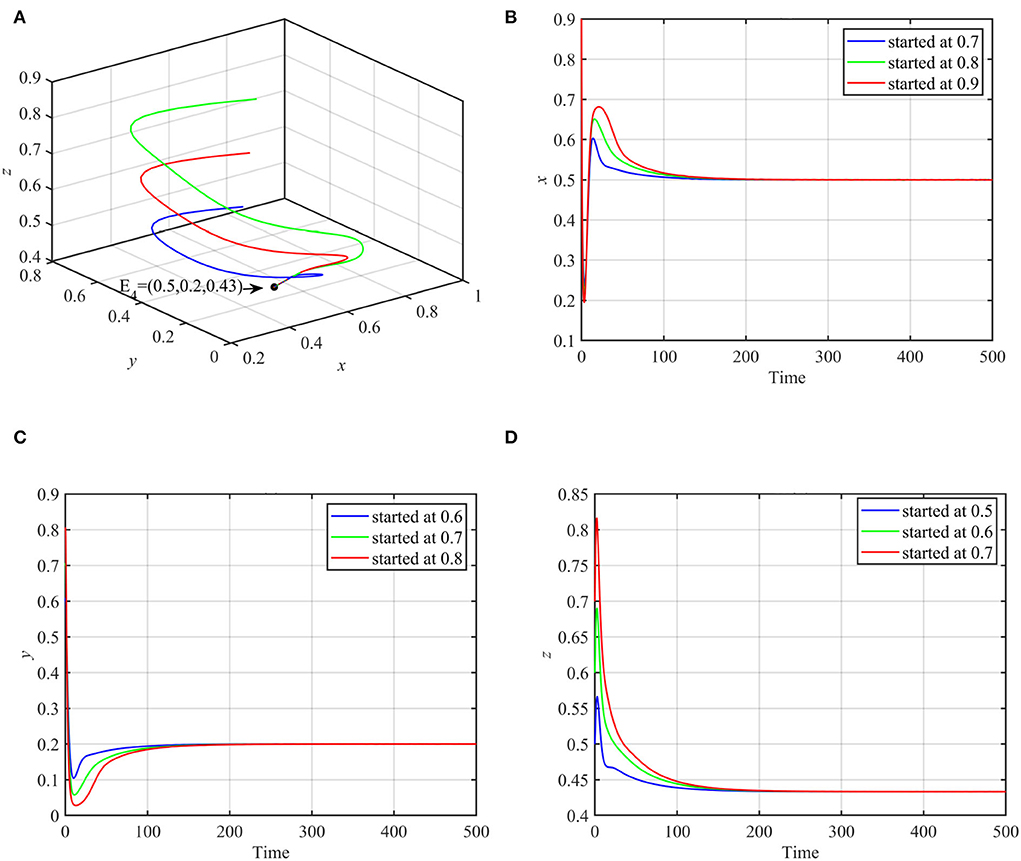
Figure 1. Globally asymptotically stable coexistence equilibrium point using data (17) and multiple initial conditions. (A) 3D-Phase portrait of the system (1). (B) Time series for trajectories of x. (C) Time series for trajectories of y. (D) Time series for trajectories of z.

Next, we varied specific parameters to understand the effect of that parameter on the dynamical behavior of the system. For the values of the parameter r satisfying r ≥ 1.84 and other parameters as in equation (17), system (1) approaches the specialist-free equilibrium point, as shown in Figure 2A for the typical value r = 2. For r ≤ 0.76 and other parameters as in equation (17), system (1) asymptotically approaches the superpredator-free equilibrium point, as shown in Figure 2B.

FIGURE 2

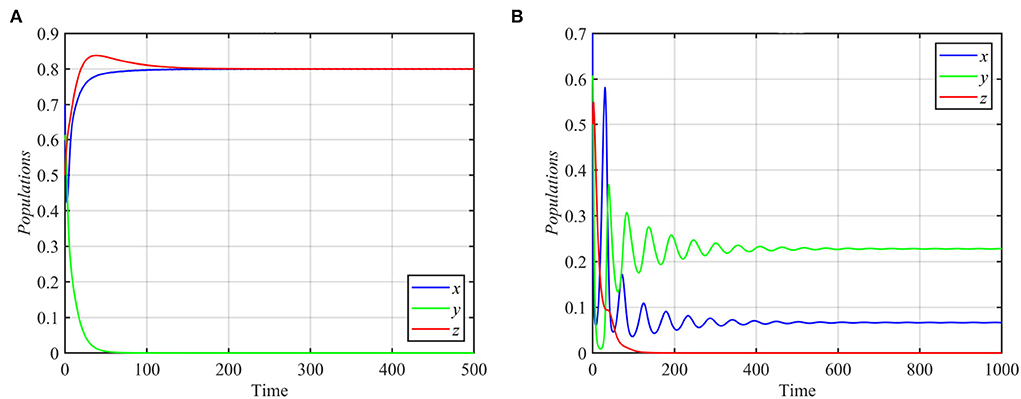
Figure 2. Trajectories of system (1) for different values of r, with other parameters as in equation (17). (A) Time series for trajectories of x, y, and z for r = 2, which approach E₂ = (0.8, 0, 0.8). (B) Time series for trajectories of x, y, and z for r = 0.3, which approach E₃ = (0.06, 0.22, 0).

For different values of the fear rate k with the rest of the data as given in equation (17), system (1) is solved numerically and illustrated in Figure 3.

FIGURE 3

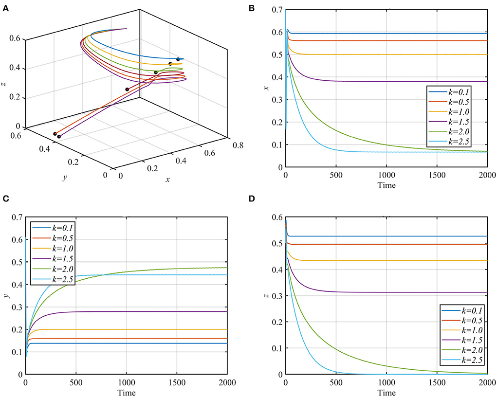
Figure 3. Trajectories of system (1) using data given in equation (17) with different values of k. (A) 3D-Phase portrait of system (1) for different values of k. (B) Time series for the trajectory of x, in which x decreases but remains positive as k increases. (C) Time series for the trajectory of y, in which y increases as k increases. (D) Time series for the trajectory of z, in which z decreases as k increases and approaches zero for k > 2.

As shown in Figure 2, the superpredator decreases as k increases, with extinction for k > 2. We also varied the parameter a₁ with other parameters still fixed as in equation (17). For the range a₁ ≥ 1.3, system (1) asymptotically approaches the superpredator-free equilibrium, as shown in Figure 4A for the typical value a₁ = 1.75. Conversely, system (1) approaches asymptotically to the specialist-free equilibrium point, as shown in Figure 4B for the typical value a₁ = 0.4.

FIGURE 4

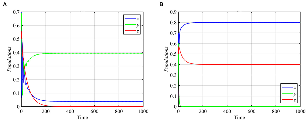
Figure 4. Trajectories of system (1) for different values of a₁ and other parameters as in equation (17). (A) Time series for trajectories of x, y, and z for a₁ = 1.75, which approach E₃ = (0.03, 0.39, 0). (B) Time series for trajectories of x, y, and z for a₁ = 0.4, which approach E₂ = (0.8, 0, 0.4).

System (1) still asymptotically approaches the coexistence equilibrium point for the data given in equation (17), when e₁ or e₃ increases or when e₂ decreases. However, for e₁ ≤ 0.44, system (1) asymptotically approaches the specialist-free equilibrium point E₂ = (0.8, 0, 0.4), as shown in Figure 4B. For e₂ ≥ 0.3 or e₃ ≤ 0.2 and the other parameters as in equation (17), the trajectories of system (1) asymptotically approach the specialist-free equilibrium point or the superpredator-free equilibrium point as shown in Figure 5.

FIGURE 5

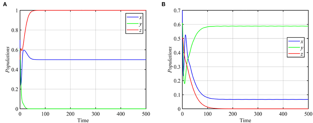
Figure 5. Trajectories of system (1) for different values of e₂ and e₃, with other parameters as in equation (17). (A) Time series for trajectories of x, y, and z for e₂ = 0.4, which approach E₂ = (0.5, 0, 1). (B) Time series for trajectories of x, y, and z for e₃ = 0.1, which approach E₃ = (0.06, 0.58, 0).

Further investigation for the effect of varying parameters a₂ and a₃ while keeping the rest of the parameters as in equation (17) shows that the parameter a₂ has similar effects as the parameter e₂ with a bifurcation point at a₂ = 0.63. However, parameter a₃ has similar effects as parameter r, with two bifurcation points: a₃ = 1.38 and a₃ = 0.62.

Finally, for d₁ ≥ 0.31 and the rest of the parameters as in equation (17), the trajectories of system (1) asymptotically approach the specialist-free equilibrium point, as shown in Figure 6A for the typical value d₁ = 0.4. However, system (1) approaches the coexistence equilibrium point otherwise. On the other hand, for d₂ ≥ 0.12 or d₂ ≤ 0.08 and the other parameters as in equation (17), trajectories of system (1) asymptotically approach either the superpredator-free equilibrium point or the specialist-free equilibrium point, as shown in Figures 6B,C for the typical values d₂ = 0.15 and d₂ = 0.08, respectively.

FIGURE 6

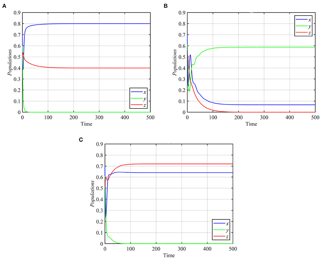
Figure 6. Trajectories of system (1) for different values of d₁ and d₂, with other parameters as in equation (17). (A) Time series for trajectories of x, y, and z for d₁ = 0.4, which approach E₂ = (0.8, 0, 0.4). (B) Time series for trajectories of x, y, and z for d₂ = 0.15, which approach E₃ = (0.06, 0.58, 0). (C) Time series for trajectories of x, y, and z for d₂ = 0.08, which approach E₂ = (0.64, 0, 0.72).

Varying parameters d₁ and d₂ together so that they satisfy conditions (7a) and (7b) while keeping other parameters as in equation (17) makes the trajectories of system (1) asymptotically approach the axial equilibrium point E₁ = (1, 0, 0) as shown in Figure 7.

FIGURE 7

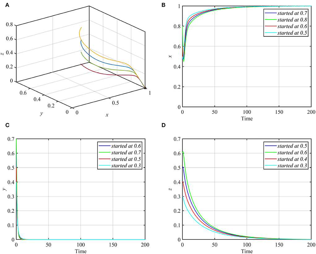
Figure 7. Globally asymptotically stable axial equilibrium point for d₁ = 0.8, d₂ = 0.15 and other parameters as in equation (17). (A) 3D-Phase portrait. (B) Time series for trajectories of x. (C) Time series for trajectories of y. (D) Time series for trajectories of z.

Discussion

Classical intraguild predation food web models have been extensively studied, but relatively little work has been done on the effect of fear on the prey. To the best of our knowledge, this is the first model considering prey fear of only the specialist predator. We determined the equilibria and global stability properties of the model, found bifurcations, and illustrated the theoretical behavior with numerical simulations.

Many previous studies have found that three-species intraguild predation models, in which a superpredator (IG predator) both attacks and competes with a specialist predator (IG prey), are often unstable, either because one consumer is excluded or because long feedback loops produce sustained oscillations [30]. Despite this, many natural IGP systems continue to thrive. Many empirical intraguild predation systems are entrenched in communities with alternative prey species, and standard models of intraguild predation simplify actual systems in significant ways that could affect persistence. Holt and Huxel [30] presented results of theoretical explorations of how alternative prey can influence the persistence and stability of a focal intraguild predation interaction. They reviewed the key conclusions of standard three-species IGP theory and then presented results of theoretical explorations of how alternative prey can influence the persistence and stability of a focal intraguild predation interaction. Conversely, Bai et al. [10] indicated that the intraguild predation food web model has rich and complicated dynamic behavior, and a large Allee effect in the basal prey raises the extinction risk of not only the basal prey but also the IG prey or/and IG predator.

Hossain et al. investigated fear in an intraguild predation model, in which the growth rate of a specialist predator (IG prey) is reduced due to the cost of fear of a superpredator (IG predator), and the growth rate of a basal prey is suppressed due to the cost of fear of both the IG prey and the IG predator [20]. In a three-species food chain system, they found that omnivory can cause chaos in the absence of fear. Fear, on the other hand, can help to keep the chaos under control. They also discovered that the system exhibits bistability between the IG prey-free and IG predator-free equilibrium, as well as bistability between IG prey-free and interior equilibria. Furthermore, they showed that the system can display numerous stable limit cycles for a given set of parameter values.

However, in our study, instilling the fear of a specialist predator (IG prey) in the presence of a superpredator (IG predator) had the unintended consequence of eradicating the superpredator. This demonstrates the often-surprising complexity of food-chain dynamics and has not been observed in previous articles dedicated to the study of fear [23–27]. In contrast, if the prey's intrinsic growth rate is sufficiently high, the IG prey can be eradicated, while the IG predator can be removed if the prey's intrinsic growth rate is sufficiently low. Coexistence or the eradication of both predators are other possibilities. As a result, system (1) has rich dynamical behavior, is sensitive to parameter changes, and at least one bifurcation point exists for each of the parameters. This result is comparable to decreasing the productivity of a resource (comparable to a higher fear effect in the prey in this manuscript) resulting in a reduction in the density of the highest trophic level [31].

The most important parameters that influenced the outcome were, in order, the growth rate r, the fear effect k, predation upon the prey by the specialist predator a₁, the conversion factor between the prey and the superpredator e₂, the conversion factor between the specialist predator and the superpredator e₃, the death rate of the specialist predator d₁, and the natural death rate of the superpredator d₂.

Our model contains several limitations, which should be acknowledged. We only looked at the prey's fear of the specialized predator, not of the superpredator, and we ignored the specialist predator's fear of the superpredator. Our interpretation of such a case is that the pressure of the superpredator on the basal prey is much lower than that of a specialist predator due to the existence of alternative food sources. Mass-action kinetics and a conversion factor are used to model each predator's attack rates, which is a simplification of the genuine dynamics. Finally, the predators were completely reliant on a single food source, which is not always the case.

As a result, the dynamics of a food web in which the prey is afraid of one predator but not the other can produce unexpected results. In the absence of other fear effects, future research will consider the prey's fear of the superpredator but not the specialized predator; the specialist predator's fear of the superpredator could also be incorporated.

Data availability statement

The original contributions presented in the study are included in the article/supplementary files, further inquiries can be directed to the corresponding author.

Author contributions

NF developed the model, wrote the initial draft, conducted analysis, and performed numerical simulations. RN conducted analysis and performed numerical simulations. MH designed the study. SS? rewrote and edited and manuscript. All authors contributed to the article and approved the submitted version.

Funding

SS? is supported by an NSERC Discovery Grant. For citation purposes, please note that the question mark is part of her name.

Conflict of interest

The authors declare that the research was conducted in the absence of any commercial or financial relationships that could be construed as a potential conflict of interest.

Publisher's note

All claims expressed in this article are solely those of the authors and do not necessarily represent those of their affiliated organizations, or those of the publisher, the editors and the reviewers. Any product that may be evaluated in this article, or claim that may be made by its manufacturer, is not guaranteed or endorsed by the publisher.

References

1. Thompson RM, Brose U, Dunne JA, Hall RO, Hladyz S, Kitching RL, et al. Food webs: reconciling the structure and function of biodiversity. Trends Ecol Evolut. (2012) 27:689–697. doi: 10.1016/j.tree.2012.08.005

PubMed Abstract | CrossRef Full Text | Google Scholar

2. Allesina S, Tang S. Stability criteria for complex ecosystems. Nature. (2012) 483:205–08. doi: 10.1038/nature10832

PubMed Abstract | CrossRef Full Text | Google Scholar

3. Aziz-Alaoui MA. Study of a leslie gower type tri-trophic population model. Chaos Solitons Fractals. (2002) 14:1275–1293. doi: 10.1016/S0960-0779(02)00079-6

CrossRef Full Text | Google Scholar

4. Gakkhar S, Singh B, Naji RK. Dynamical behavior of two predators competing over a single prey. BioSystem. (2007) 90:808–817. doi: 10.1016/j.biosystems.2007.04.003

PubMed Abstract | CrossRef Full Text | Google Scholar

5. Gakkhar S, Naji RK. On a food web consisting of a specialist and generalist predator. J Biol Syst. (2003) 11:365–376. doi: 10.1142/S0218339003000956

CrossRef Full Text | Google Scholar

6. Gakkhar S, Naji RK. Order and chaos in a food web consisting of a predator and two independent preys. Commun Nonlinear Sci Numer Simulat. (2005) 10:105–120. doi: 10.1016/S1007-5704(03)00120-5

CrossRef Full Text | Google Scholar

7. Klebanoff A, Hastings A. Chaos in one predator two prey model: general results from bifurcation theory. Math. Biosciences. (1994) 122:221–223. doi: 10.1016/0025-5564(94)90059-0

PubMed Abstract | CrossRef Full Text | Google Scholar

8. Holt RD, Polis GA. A theoretical framework for intraguild predation. Am Natur. (1997) 149:745–764. doi: 10.1086/286018

CrossRef Full Text | Google Scholar

9. Tanabe K, Namba T. Omnivory creates chaos in simple food web models. Ecology. (2005) 86:3411–3414. doi: 10.1890/05-0720

CrossRef Full Text | Google Scholar

10. Bai YK, Ruan S, Wang L. Dynamics of an intraguild predation food web model with strong Allee effect in the basal prey. Nonlinear Anal Real World Appl. (2021) 58:103206. doi: 10.1016/j.nonrwa.2020.103206

CrossRef Full Text | Google Scholar

11. Sabelis MW. Predatory arthropods. In: Natural enemies, the population biology of predators, parasites and diseases, eds M. J. Crawley (Oxford: Blackwell Scientific) (1992). p. 225–264. doi: 10.1002/9781444314076.ch10

CrossRef Full Text | Google Scholar

12. Crowder DW, Snyder WE. Eating their way to the top? Mechanisms underlying the 456 success of invasive generalist predators. Biol Invas. (2010) 12:2857–2876. doi: 10.1007/s10530-010-9733-8

CrossRef Full Text | Google Scholar

13. Schreiber SJ. Generalist and specialist predators that mediate permanence in ecological communities. J. Math. Biol. (1997) 36:133–148 doi: 10.1007/s002850050094

CrossRef Full Text | Google Scholar

14. Lima S, Dill LM. Behavioral decisions made under the risk of predation: a review and prospectus. Can. J. Zool. (1990) 68:619–640. doi: 10.1139/z90-092

CrossRef Full Text | Google Scholar

15. Panday P, Pal N, Samanta S, Chattopadhyay J. Stability and bifurcation analysis of a three-species food chain model with fear. Int J Bifurcation Chaos. (2018) 28:1850009. doi: 10.1142/S0218127418500098

CrossRef Full Text | Google Scholar

16. Clinchy LMDi, Roberts D, Zanette LY. Fear of large carnivores causes a trophic cascade. Nat Commun. (2016) 7:10698. doi: 10.1038/ncomms10698

PubMed Abstract | CrossRef Full Text | Google Scholar

17. Panday NP, Samanta S, Chattopadhyay J. A three species food chain model with fear induced trophic cascade. Int J Appl Comput Math. (2019) 5:1–26. doi: 10.1007/s40819-019-0688-x

CrossRef Full Text | Google Scholar

18. Panday P, Samanta S, Pal N, Chattopadhyay J. Delay induced multiple stability switch and chaos in a predator–prey model with fear effect. Math Comput Simulat. (2020) 172:134–58. doi: 10.1016/j.matcom.2019.12.015

CrossRef Full Text | Google Scholar

19. Cong MF, Zou X. Dynamics of a three-species food chain model with fear effect. Commun Nonlinear Sci Numer Simulat. (2021) 99:105809. doi: 10.1016/j.cnsns.2021.105809

CrossRef Full Text | Google Scholar

20. Hossain NP, Samanta S, Chattopadhyay J. Fear induced stabilization in an intraguild predation model international. J Bifurcation Chaos. (2020) 30:2050053. doi: 10.1142/S0218127420500534

CrossRef Full Text | Google Scholar

21. Mukherjee D. Role of fear in predator–prey system with intraspecific competition. Math Comput Simulat. (2020) 177: 263–275. doi: 10.1016/j.matcom.2020.04.025

CrossRef Full Text | Google Scholar

22. Ibrahim HA, Naji RK. Chaos in beddington–deangelis food chain model with fear. J Phys Conf Ser. (2020) 1591:012082. doi: 10.1088/1742-6596/1591/1/012082

CrossRef Full Text | Google Scholar

23. Mondal B, Roy S, Ghosh U, Tiwari PK. A systematic study of autonomous and nonautonomous predator–prey models for the combined effects of fear, refuge, cooperation and harvesting. Eur Phys J Plus. (2022) 137:724. doi: 10.1140/epjp/s13360-022-02915-0

PubMed Abstract | CrossRef Full Text | Google Scholar

24. Roy S, Tiwari PK, Nayak H, Martcheva M. Effects of fear, refuge and hunting cooperation in a seasonally forced eco-epidemic model with selective predation. Eur Phys J Plus. (2022) 137:1–31. doi: 10.1140/epjp/s13360-022-02751-2

CrossRef Full Text | Google Scholar

25. Maity PKTi, Pal S. An ecoepidemic seasonally forced model for the combined effects of fear, additional foods and selective predation. J Biol Syst. (2022) 12:1–37. doi: 10.1142/S0218339022500103

CrossRef Full Text | Google Scholar

26. Pal PKTi, Pal N. Bifurcations, chaos, and multistability in a nonautonomous predator–prey model with fear Chaos: an interdisciplinary. J Nonlinear Sci. (2021) 31:123–34. doi: 10.1063/5.0067046

PubMed Abstract | CrossRef Full Text | Google Scholar

27. Tiwari PK, Verma M, Pal S, Kang Y, Misra AK. A delay nonautonomous predator–prey model for the effects of fear, refuge and hunting cooperation. J Biol Syst. (2021) 29:927–69. doi: 10.1142/S0218339021500236

CrossRef Full Text | Google Scholar

28. Wang X, Zanette L, Zou X. Modelling the fear effect in predator–prey interactions. J Math Biol. (2016) 73:1179–1204. doi: 10.1007/s00285-016-0989-1

PubMed Abstract | CrossRef Full Text | Google Scholar

29. Perko L. Differential Equations and Dynamical Systems, Volume 7. New York: Springer (1996). doi: 10.1007/978-1-4684-0249-0

CrossRef Full Text | Google Scholar

30. Holt RD, Huxel GR. Alternative prey and the dynamics of intraguild predation: theoretical perspectives. Ecology. (2007) 88:2706–2712. doi: 10.1890/06-1525.1

PubMed Abstract | CrossRef Full Text | Google Scholar

31. Gurney W, Nisbet RM. Ecological Dynamics. Oxford: Oxford University Press. (1998).

Google Scholar

Keywords: intraguild predation, food web, fear effect, stability, specialist predator

Citation: Fakhry NH, Naji RK, Smith? SR and Haque M (2022) Prey fear of a specialist predator in a tri-trophic food web can eliminate the superpredator. Front. Appl. Math. Stat. 8:963991. doi: 10.3389/fams.2022.963991

Received: 08 June 2022; Accepted: 05 October 2022;
Published: 03 November 2022.

Edited by:

Aurelio A. de los Reyes V, University of the Philippines Diliman, Philippines

Reviewed by:

Pankaj Tiwari, University of Kalyani, India
Abdelalim A. Elsadany, Suez Canal University, Egypt

Copyright © 2022 Fakhry, Naji, Smith? and Haque. This is an open-access article distributed under the terms of the Creative Commons Attribution License (CC BY). The use, distribution or reproduction in other forums is permitted, provided the original author(s) and the copyright owner(s) are credited and that the original publication in this journal is cited, in accordance with accepted academic practice. No use, distribution or reproduction is permitted which does not comply with these terms.

*Correspondence: Mainul Haque, Mainul.Haque@nottingham.edu.cn

ORIGINAL RESEARCH article

Prey fear of a specialist predator in a tri-trophic food web can eliminate the superpredator

Introduction

Food-web model formulation

Existence of equilibrium points

Persistence

Global stability analysis

Bifurcation analysis

Numerical simulations

Discussion

Data availability statement

Author contributions

Funding

Conflict of interest

Publisher's note

References

This article is part of the Research Topic

People also looked at