Application of Copulas to Improve the Modeling of Housing Tenure and Affordability
 Emmanuel Kabundu
 Brink Botha2
 - 1Department of Building and Human Settlements Development, Nelson Mandela University, Port Elizabeth, South Africa
- 2Department of Construction Management, Nelson Mandela University, Port Elizabeth, South Africa
- 3Department of Building and Human Settlements Development, Nelson Mandela University, Port Elizabeth, South Africa
- 4Department of Quantity Surveying, Nelson Mandela University, Port Elizabeth, South Africa
The tenure statuses made by households (renter-occupancy or owner-occupancy) are influenced by a multitude of factors, some of which cannot be directly measured. However, economists are still interested in knowing the relative severity and patterns of influence these factors have on housing tenure status. The purpose of this research was to determine the effect of assuming joint dependency between housing tenure and affordability on the model results. The effect of model-mis-specification on severity and relative importance of the explanatory variables was also assessed. Joint bivariate binary regression was applied to multi-year cross-sectional General Household Survey (GHS) data from Statistics South Africa (STATSA). An assumption of a univariate model when modeling both housing affordability and tenure led to model mis-specification, because most of the coefficients between the univariate and bivariate joint models were significantly different. Model mis-specification also led to significant differences in rankings of the levels of influence of the explanatory variables. Bivariate joint modeling with appropriate error-model copulas improved the model results. Older households that were above 49 years were consistently more likely to be owner-occupiers, and the household head age variable for older households was the most influential factor for housing owner-occupancy and affordability.
Introduction
The housing tenure statuses by households (renting or owner-occupancy) are influenced by a multitude of factors, some of which cannot be directly measured [1]. Though it is neither possible nor practical to measure and include all the explanatory variables that influence housing tenure and affordability, economists are still interested in studying the patterns and levels of influence of any available measurable explanatory variables (for example [2–5]).
Several studies have modeled housing tenure based on univariate modeling. Some of these studies preferred to use probit models, where the underlying distribution is considered a normal distribution. However, the assumption of normality is not based on proper justification. Therefore, some studies have opted to use other binary link functions such as the logit function, which assumes a more flexible logistic distribution. However, the methods used in these studies do not allow for joint modeling, where dependence is assumed to exist between the binary responses [4, 6–8]. Other studies (such as [2, 5]) which have assumed existence of joint dependence (with one of the responses being housing tenure), have employed a 2 or 3-stage least squares method (that uses structural equation modeling) to model the responses. The least-squares method is, however, not good for modeling in scenarios where the binary response variables are involved [9]. Furthermore, the least squares method is only applicable where linear relationships are assumed and the estimates made are possible only about the mean [10, 11].
This paper sets out to determine whether the assumption of reverse causality between housing tenure and affordability is justified during modeling. The study will determine if the use of a bivariate binary joint model (with endogenous treatment) is better than a univariate binary model for housing tenure and affordability [12]. The most influential variables and corresponding patterns of influence, will be determined. This kind of modeling allows for dealing with unobserved confounding and non-Gaussian dependencies between treatment and outcome [12]. This paper adds value to current research in that, in contrast to previous studies, it approaches the modeling of housing tenure and affordability by assuming possible joint dependency between the two responses, and possible presence of non-Gaussian copula error models. The resulting model if justified would be a significant model improvement compared to previous models.
The paper is divided into the following sections: Section (ii) will deal with the housing tenure and affordability context in South Africa. It will also explore various factors that have been identified to influence housing tenure and affordability from previous studies. Section (iii) will discuss the methodology. Section (iv) will present the results while section (v) will deal with the discussion of the results. Finally, section (vi) will summarize the contribution of the paper to existing knowledge and propose future areas for further research.
Background
Factors That Influence Housing Affordability and Tenure
Housing affordability: Studies that identify factors that influence housing affordability are mostly not based on regression modeling methodology or are based on the univariate modeling regression methodology. However among the factors that influence housing affordability include housing-tenure, demographic factors, migration, location, race, time, planning and zoning, living conditions, income inequalities, ownership of land, rents, government policy, income, race, education, and household size [13, 14].
Housing tenure: Various factors have been identified as relevant for inclusion in modeling housing tenure and affordability. Research done using multi-level logistic regression in China used age, marital status, education level of household head, household income, household size, number of workers in the household, building price, nature of job held and locational factors as the variables influencing tenure. Both market mechanisms and institutional factors affected housing tenure in urban areas of China. Social-economic factors such as age, household size and income and house price had similar effects as in the western countries. The factors related to education and some factors related to employment were the ones that did not turn out to be significant at the 5% level [6]. On the other hand, Liao and Zhang [15] also carried out research in China and used various models, including ordinary least squares, two-stage least squares, probit and bivariate probit models. The level of significance was again 5%. The locational factors, age, marital status, years of education, household income, and employment in the government sector were used. All factors were significant for all the models except the government employment factor concerning the two-stage least squares model and one of the ordinary least squares models.
Tandoh and Tewari [7] used the logistic regression to model tenure in Ghana by using income, house price index, household size, marital status, gender, employment status of household head, value to rent ratio and urban locational status of the household. The value to rent ratio, highest education at university and highest education at secondary school were all not significant at 5% level. The rest of the factors were significant.
In his research in the United States of America (USA), Carter [2] emphasized the need to control for endogeneity when modeling housing tenure-of-choice with respect to the second household income. The methodology used involved use of the 2-Stage least squares method (2SLS). The results showed that the probability of homeownership was increased by 4–6% when modeling is not controlled for endogeneity. When endogeneity was controlled for (using least squares and probit regression in two stages), all variables were significant at the 5% level except the Metropolitan Statistical Area median rent values. The variables included the wife's income, permanent income, the number of children, the wife's age, the combined tax rate of the couple, the house price index and locational factors.
Spalkova and Spalek [4] also researched to find out the factors that influence housing tenure-of-choice in the Czech Republic using the logit model. The data consisted of an annual cross-sectional survey for 5 years. The variables included income, proportion of household members in various age categories, locational factors, floor area per person, gender, marital status, employment status, work status, age, and educational status of the household head. All variables were significant at the 5% level except a few variables related to the proportions of household members in certain age categories for some years. The study indicated that apart from income, tenure is also significantly influenced by household size and location in Prague, the capital of the Czech Republic. The study indicated that Prague households are more likely to be renters than owner-occupiers.
Bazyl [3] also investigates the factors influencing housing tenure in other European countries. The study indicated that marriage was generally a significant determinant of switching from renting to owner-occupancy. Other factors that were significant in some countries but not in others included the nationality, income, and age of the household head.
Summary: The above studies indicate that most factors that influence housing affordability also influence housing tenure. Careful examination of the studies also reveals that housing affordability seems to influence housing tenure. On the other hand, housing tenure also influences housing affordability.
South Africa
Historical context of tenure: Land tenure consists of the terms and conditions under which land is held, used and transacted and is a major determinant in both the management of resources and distribution of benefits [16]. From 1913 up to 1991, the South African history of ownership of property rights was shaped by a series of Acts of Parliament that encouraged territorial segregation based on race, and prohibited natives from occupancy or acquisition of land in some designated areas. Urban areas are typical examples where these restrictions once applied. But the restrictions also extended into other areas such as rural and farming areas. The Natives Land Act 27 of 1913, for example reserved only <10% of South African land for Blacks. The Native Trust and Land Act 18 of 1936, had an aim of abolishing individual land ownership by Black natives and introduced trust tenure through the South African Development Trust. This Government body would acquire land only in specially “released areas” for settlement by native Black South Africans [17–19].
The Group Areas Act 41 of 1950 and the Group Areas Act 36 of 1966 are other instruments that were introduced by the then existing Government, that ultimately established group areas according to race (Native Black, Colored, Asian, and White areas) and prohibited both land acquisition and land occupation by any race in any area which was not allotted to that particular race. It enforced residential and commercial segregation in urban areas. These Acts led to forced evictions of about 3.5 million people between 1960 and 1983 [17, 20, 21]. The segregation therefore negatively affected Natives, Coloreds and Asians with respect to freedom of acquisition of property rights, occupation and ability to conduct business.
It was against this backdrop of almost 80 years of restricted occupancy and property ownership which was heavily biased against Black, Asian and Colored South Africans, that it was necessary to introduce the “Abolition of Racially Based Land Measures Act 108 of 1991”. This Act both abolished the previous four (4) Acts and phased out the South African Development Trust [22]. The new Government in 1994 was faced with the problem of high incidence of poverty among most of the South African households because of the iniquities related to property ownership that had been in place for almost 80 years. A direct consequence of this is that, while urban real estate is one of the major assets in which wealth is vested within South Africa, 90–95% of South African wealth is owned by just 10% of the population, majority of whom are white population that were not negatively affected by segregationist policies. As a result, there are persistent severe high income inequalities in South Africa [17, 23].
It was therefore necessary to introduce extensive housing subsidy programs that would help to alleviate poverty and, to an extent, improve the quality of life for as many of the previously marginalized communities as possible. One such a program was the Reconstruction for Development Program (RDP) that was aimed at providing housing subsidies through provision of complete housing units to such households. The program in its improved format ensures that the location of the homes are in economically strategic areas, through an integrated human settlements approach [24, 25].
Major forms of tenure: Land tenure systems in South Africa can be broadly categorized into Privately owned land (72% of total), State owned land (14% of total) and Customary owned land (14% of total) systems [16]. If permanent improvements are taken into consideration, the various classification of individual forms of housing tenure include the freeholds, time shares, permission to occupy (PTO), Leaseholds (short and long term leases), block shares and sectional titles [26]. Freehold involves perpetual ownership of land and buildings, whereby the ownership rights are registrable at the Deeds Registry (end result is a registered title deed). A freehold owner possesses the most comprehensive rights in property, subject to the laws and regulations from the respective Government. In a sectional title form of ownership, the land and some permanent improvements that are shared by all occupants (such as parking areas, walkways and lifts) are taken to be under common ownership while most of the permanent improvements on the land mostly consist of individually owned sections. Ownership of each section and the corresponding undivided share in common property, whose size depends upon the participation quota, is registrable under a title deed [26, 27].
A leasehold grants the lessee almost the same benefits of a freehold owner, but only for a limited time. While leaseholds do not confer ownership to lessees, long term leases (>10 years) need to be registered in South Africa. In a share block, a single company may own a given property and an individual is allowed to buy the rights to use a specific unit by buying shares in the company. There is no title granted to an owner of a share block, but he only obtains a creditor's right against the share block company to use a certain part of the building, as specified in the Share Blocks Control Act 59 of 1980. According to the South African Time Shares control Act 75 of 1983, a time share provides the holder of the time share unit the right to use such a unit for a given period annually. The holder of a time share could be such by virtue of co-ownership of the accommodation or could be a lessee under a time-share developer [28]. A time share holder, therefore, may or may not hold a title deed over the time share property under consideration. On the other hand, the permission to occupy (PTO) is a right granted by Government to certain types of rural and unsurveyed land, but may be revoked by the Government after consultation with tribal authorities. Since the holder is given the right to live on the land, he can erect permanent improvements such as a house on that land, but cannot obtain a title deed against such a property. While such a right is registrable in some departments in South Africa, it is not registrable in the Deeds Registry, and appears insecure. Currently, tribal authorities are, instead, expected to provide more secure forms of tenure with a formal title deed. Alternatively, some existing PTO's have been converted to long term leases [26, 29, 30].
In 2017, while 94% of all land in South Africa was registered in the Deeds Registry, 6% was not registered but was in the process of being surveyed, registered and given to individual and community owners. On the other hand, while urban land accounted for 3% of the total land area of the Country, the number of parcels in urban areas comprised of 94% of all land parcels in South Africa and were owned by 93% of all land owners [31]. This highlights the significantly higher economic utility and locational rent possessed by urban land, in comparison with non-urban land in South Africa.
For data collection purposes with respect to their surveys, the major forms of tenure in South Africa, as indicated by STATSA [32], however, include housing units rented from private individuals, housing units that are owned but not fully paid off to financial institutions, housing units that are rented from the municipalities or social housing institutions, housing units that are owned but not fully paid off to a private lender, housing units that are owned but fully paid off, and housing units that are occupied, but rent-free. The households staying in housing units which they owned, irrespective of whether they have fully paid them off or not, will be classified here as owner-occupiers. The households that are renting housing units (irrespective of the type of landlord) or are occupying housing units that are not theirs, but without paying rent permanently or temporarily will be classified as renter-occupiers.
Housing market: The housing market, however, can be broadly categorized into private sponsored housing and government-sponsored housing. Each of these two (2) forms of housing can be further categorized into owner-occupied and rent-occupied housing. Government-sponsored housing based on subsidies (finance-linked and non-finance-linked) is usually targeted from low-income groups up to lower-middle-income groups. There are sixteen (16) National Housing Programmes that benefit from the housing subsidies [24]. Prominent among these 16 is the Individual Subsidy Programme (ISP), which provides access to funding of individual house ownership in the form of either a credit-linked (finance linked) or non-credit linked subsidies [24]. The demand for owner-occupied housing (both government-sponsored and privately sponsored) has historically outstripped the housing supply in South Africa, resulting in an ever-increasing housing backlog, especially since 2010 [33]. It has been exacerbated by the effects of the global COVID pandemic and its associated lockdown phases that have negatively impacted the South African economy. According to estimates, the South African economy contracted by about 7.0% in 2020, mainly owing to Covid-19-related lockdown measures [34]. This has also meant limited household access to funds from both the government housing subsidies and the private sector.
Trends: Before 2020, the historical data related to owner-occupancy and renting in south Africa already was showing a steadily increasing proportion of renter-occupiers in South Africa. However, the housing market was still biased toward owner-occupancy. This trend was evident across all provinces, with Gauteng province (Gauteng is the most urbanized province, followed by the Western Cape) which consistently had the highest proportions of renters, increasing from 30.2% in 2009 to 36.2 % in 2018. The corresponding figures for Western Cape were 24.4% in 2009 and 31.8% in 2018 [32, 35]. This indicates a steady decline in the affordability of owner-occupancy, with the eventual alternative being renter-occupancy.
Though accurate data for 2020 and 2021 is not available, a poor performing economy during this period may have shifted the housing market still further toward renter-occupancy. At any rate, evidence strongly indicates that renting is becoming ever more important to the South African household across all provinces.
Methods
Housing Affordability and Tenure Modeling
Housing affordability is that which is concerned with securing some given standard of housing (or different standards) at a price or a rent which does not impose (in the eyes of some third party; usually, but not always the government) an unreasonable burden on household incomes [36]. Housing affordability can be measured based on ratios of housing expenses to income as applied in percentage-of-income method [37]. Therefore, housing affordability can be considered equivalent to the ratio of monthly mortgage or rent payments to the monthly household income. The following formulas apply:
Where:
• Gm represents the monthly mortgage
• Tm represents the monthly rent
• Cm represents the monthly income
• fown represents the affordability ratio for owner occupancy
• frent represents the affordability ratio for renter occupancy
These housing affordability ratios can be transformed into binary formats since financial institutions in South Africa consider households that have ratios equal to or below 0.3 or thirty per cent (30%) not to have affordability problems (These ratios are assigned a value of one), while households with ratios above thirty per cent (30%) have affordability problems (these are assigned a value of zero). The explanatory variables can be factors such as household incomes, household head age category, dummy variables, household size, provincial location dummy variables, the household metro location dummy, household head age, gender, the household subsidy status, house values and the household head race [32, 35, 38–40]. The housing tenure response variable can also be assigned binary values in such a way that if a household was an owner-occupier, then it would be assigned a value of one (1). If the household were renter-occupiers, it would be assigned a value of zero (0).
Binary regression modeling (probit, logit, or cloglog modeling) would be the best form of modeling in a case where both housing tenure and affordability are expressed as binary variables. Probit models are a form of binary choice models used when the dependent variable in a mathematical model is binary in nature, and the errors for the log linearized model are normally distributed. If the errors follow a standard extreme value distribution or double exponential distribution, then the appropriate mathematical model for use would be a complementary log- log or the cloglog model. On the other hand, if the errors follow a standard logistic distribution, then the appropriate mathematical model for use is a logit model [41]. Thus, by assigning the outcome of owner occupancy to be one (1) and renter occupancy to be zero (0), it is possible to construct a probit, logit, or cloglog model and conduct housing tenure and affordability-based analysis on appropriate household data.
The Bivariate Binary Joint Regression Model
A joint Bivariate binary regression model was proposed for use. The first equation, which corresponds to housing affordability as the response variable, is the endogenous treatment equation. The second equation that corresponds to housing tenure is the outcome equation that receives the treatment. It is assumed that yai and yti are a pair of binary random variables for housing affordability and tenure, respectively. We shall also assume that i=1 to n, whereby n is the sample size from which yai and yti are drawn. The corresponding linear predictors for housing affordability and tenure are denoted as ηai and ηti. It follows that yai = 1 when ηai > 0 and yti = 1 when ηti > 0.
The linear predictor corresponding to the endogenous treatment equation (affordability) is given in Equation (3) below.
The linear predictor for the outcome equation (tenure) is given in Equation (4) below.
The term φ is a measure of the effect of the treatment (affordability) on the outcome (housing tenure) based on the scale of the linear predictor. The term Zai is a vector that contains parameters (such as intercept, dummy, and categorical variables). The term βa is a vector that contains the coefficients to the parameters in Zai [42]. Therefore, there are 2 forms of endogeneity that are of interest. The first form is due to the omitted or non-included terms in each of the equations. The second form is due to the association or interdependency (reverse causality) between each of the response variables. The model that best suits this kind of assumption is the bivariate binary regression model with endogenous treatment as represented in Equations (3) and (4).
The model is completed by including a linear predictor (ηci) for the association parameter. Equation (5) represents the equation for this linear predictor.
Where ηci is the additive predictor for the copula representing the bivariate error model. Because of the introduction of the copula model equation, the error terms εwi and εti become part of the copula model equation.
The Degree of Association (Association Parameter and Kendall's Tau)
One of the outputs of the joint modeling is an association parameter (theta or θ), whose magnitude of departure from zero (0) is a measure of the strength between housing affordability and housing tenure [43, 44]. A high association parameter is an indicator of a high dependence between housing affordability and housing tenure. From Equation (5), the association parameter θ = mηci, where m is a scaling factor that is applied to ensure that θ falls within the required range [12]. The association parameter can be transformed into Kendall's Tau for easier interpretation. The transformation varies according to the selected copula and the binary pair link function being used [45]. The interpretation of Kendall's Tau is as follows:
• If Tau is less or equal to 0.10, the association is very weak.
• If Tau is >0.10 but less than or equal to 0.19, the association is weak.
• If Tau is >0.19 but less than or equal to 0.29, the association is moderate.
• If Tau is >0.29, the association is strong.
Design
Pseudo-panel secondary data from field surveys conducted by STATSA was used for 2015, 2016, 2017, and 2018. These datasets included both housing subsidy beneficiaries and housing subsidy non-beneficiaries. Conditions for beneficiaries are specified under the Reconstruction for Development Programme (RDP) in the National Housing Code [24]. Once the datasets were cleaned, the research set out to accomplish the following tasks:
• Two model equations will be formulated and variance inflation factors will be computed to test for multicollinearity. The Akaike information criteria (AIC) will be used to test for the best bivariate error model.
• The datasets will be transformed (scaled), and scaled models will be computed. The mean of the coefficients will then be evaluated a comparison of their relative influence on the response variables (housing affordability and housing tenure) will be made.
• The rankings of the relative importance of the scaled coefficients will be made for both the univariate and bivariate models in order to evaluate how severely the model mis-specification affects the relative importance of the explanatory variables.
• Statistical tests will be done to test for the significance of the differences between the values of the univariate model coefficients and the values of the bivariate model coefficients.
Sampling
Statistics South Africa did a multi-stage sampling. It was based on a stratified design, with the stratification being based on the primary unit sizes, the geography, and the characteristics of the population [32, 38–40]. The population consisted of all the households in South Africa. The sample sizes for the data used correspond to the General Household Survey sample sizes for the respective years (2018, 2017, 2016, and 2015).
Instrument Design and Data Collection
The questionnaire was developed and administered by Statistics South Africa. Therefore, the data collected was secondary data (General Household Survey data) from Statistics South Africa. Field staff members were trained by Statistics South Africa on how to administer the questionnaires. The metadata files for the General Household Surveys have the detailed descriptions of the fields for the questionnaire used for each respective survey. It was ensured that the trained staff members were on hand to assist householders to fill in the questionnaires [32, 38–40].
Parameter Interpretation and the Equations
Table 1 presents the parameter (variable) interpretation for all the parameters used in the binary joint regression modeling equations.
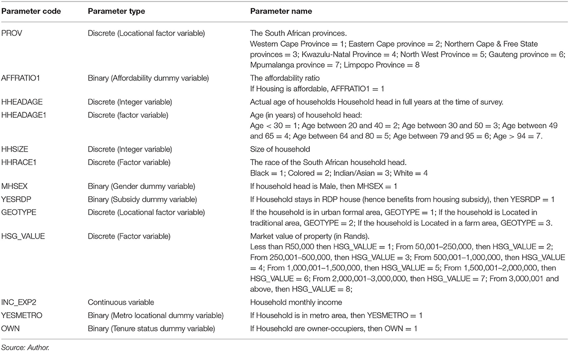
Table 1. Variable interpretation.
The implications of housing affordability influencing housing tenure and vice versa (reverse causality) are that if housing tenure is a response variable, then housing affordability must be one of its corresponding explanatory or anteceding variables. Alternatively, if housing affordability is a response variable, then most of the explanatories corresponding to housing tenure must also be the corresponding explanatory or anteceding variables for housing affordability. The solution to this kind of problem would be a bivariate binary joint regression model, with endogenous treatment being received by housing tenure from housing affordability [12]. This modeling is implemented in the Generalized Joint regression modeling (GJRM) package [44, 46]. The following Equations (6) and (7) were used for the bivariate binary joint modeling.
Equation (6) is the implementation of Equation (3) using GJRM package in R. Equation (7) is the implementation of Equation (4) using the GJRM package in R. The second Equation (7) describes the binary outcome of housing tenure or “OWN” as a function of the binary treatment or housing affordability. The first Equation (6) determines whether the endogenous treatment is received. The parameter vector estimate is obtained by using the penalized maximum likelihood method. Other covariates were also included in the model. It was assumed that the latent errors of the two equations followed a bivariate joint distribution (according to Equation 5) having an association parameter called theta (θ). The evaluation of the association parameter is preceded by the selection of an appropriate copula for the bivariate binary error model (based on AIC), as described earlier [12].
Data Analysis
Summary statistics for each dataset corresponding to each year were computed, and missing data analysis was first carried out with the help of the finalfit package of R, followed by a computation of reliability measures [47–49]. For categorical or dichotomous data, polychoric correlations were used rather than Pearson's correlations [50]. The copula methods inherent in GJRM are, however, very effective in dealing with datasets that have missing not at random (MNAR) data, with tolerances of up to 50% of missing data [51]. Precautions were taken not to include explanatory variables that are strongly correlated together on the same side of the regression equations during the formulation of the regression formulae. Variance inflation factors (VIF) were evaluated to detect this phenomenon of multicollinearity. For interpretation purposes, the following information was used.
• If VIF was equal to 1, then there was no correlation.
• If VIF was between 1 and 5 then the correlation was moderate.
• If VIF was 5 and above, then there was a high correlation. A higher VIF value indicates a higher corresponding multicollinearity with respect to the independent variable.
The Akaike information criteria (AIC) are then used to determine the best bivariate error model. The binary regression models were then generated, using the bivariate error model with the lowest AIC value for each dataset [44].
Scaling the Coefficients
To perform an analysis of the relative importance of the factors that influence housing tenure and affordability, it was necessary to scale the datasets, and hence use the scaled coefficients. Gelman [52] proposed scaling that involves subtracting the mean and dividing by twice the standard deviation of the data field elements in question. Equation (8) illustrates this:
Where:
“Xs” is the scaled version of the observation corresponding to observation “X”.
“m” is the mean of the variable representing the X-values.
“sd” is the standard deviation of the variable representing the X-values.
Logistic Coefficients and Their Interpretation: Conditional Odds Ratio
The exponents of the logit coefficients provide conditional odds ratios for the occurrence of homeownership. In this case the conditional odds ratio is the ratio of occurrence of homeownership to the non-occurrence of homeownership, given that the occurrence is caused by a unit increase in the explanatory variable in question [change of affordability ratio from a value less or equal to thirty per cent (30%) to a value greater than thirty per cent (30%)], assuming the other explanatory variables other than the explanatory variable under consideration are constant. The conditional probabilities for the occurrence of homeownership can be derived from the conditional odds ratios. The equation for their derivation is shown as Equation (9):
where “pc” is the conditional probability of homeownership, and “ORc” is the conditional odds ratio. The results for the logit-logit link pair with respect to both housing tenure and affordability modeling were then tabulated [44].
Significance of Differences in Coefficients Between the Univariate and Bivariate Models
In order to evaluate how the differences in modeling housing tenure and affordability will affect the individual coefficients (excluding the constant term), z-scores will be computed to test if the respective coefficients in each of the models are equal. Equation (10) was used to generate the z-score [53].
The values β are coefficients for variable “i.” The values s are the standard errors of the coefficients for variable “i.” The symbols b and u represent the bivariate joint binary model and the univariate binary model, respectively. The value z represents the z-statistic. Using the z-statistic, the p-values for each coefficient are computed and compares to the 5% level of significance. The null hypothesis (H0) is that the value of a given coefficient in the bivariate joint binary model is equal to the value of its corresponding coefficient in the univariate binary model. The alternative hypothesis (HA) is that these two values are not equal. A two-tailed test is then carried out. If the p-value is <5% the null hypothesis is rejected in favor of the alternative hypothesis, and vice versa.
Ethical Considerations
The identity of the participants or households in the publicly available general household survey datasets was hidden, and the data collected was used only for the research for which it was intended. This agreed with recommended ethical principles [35, 54]. Therefore, the likely damage to the households due to the re-use of the data as secondary data was non-existent. The research was also in compliance with relevant South African data protection and access policies.
Results
All initial datasets were large (sample sizes 20,908 for 2018; 21,225 for 2017; 21,218 for 2016 and 21,601 for 2015) and were appropriate to be used for regression despite instances of missing data. The percentages of missing data after cleaning the datasets were 8.9% for 2018, 14.9% for 2017, 8.3% for 2016, and 7.8% for 2015. This corresponded to final sample sizes of 19,042 for 2018; 18,060 for 2017; 19,466 for 2016, and 199,24 for 2015. Therefore, the highest instance of missing data was 14.9% in 2017. On the other hand, the GJRM copula routines have been tested and can tolerate missing data of up to 50% [51]. Although a missing data analysis was carried out, there was no necessity to present its results because the worst scenario dataset had about 14.9% missing data, which was within the tolerance limits of the GJRM. The omega total values were classified as “good.” The values for omega-total were 0.81, 0.88, 0.90, 0.90, and 0.97 for the years 2015–2018, respectively. Table 2 shows the AIC values for the bivariate error models based on the logit-logit pair link function. The best bivariate error model for 2018, 2017, and 2015 was the Student-T copula model. The best bivariate error model for 2016 was the Joe copila model.
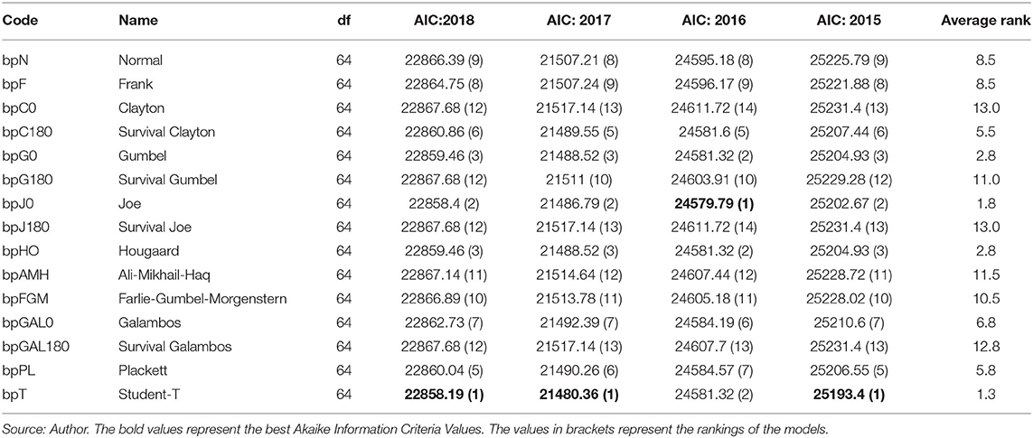
Table 2. Ranking of bivariate error models based on AIC.
Variance Inflation Factors for Multicollinearity (VIF)
Table 3 shows the mean, maximum, minimum and standard deviations of the VIF factors evaluated for each dataset with respect to housing affordability and tenure as responses. All the VIF values were consistently below 5. Therefore, there was moderate or low correlation.
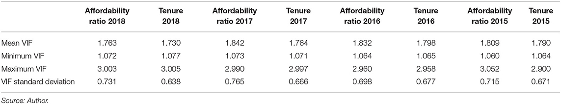
Table 3. Summaries of VIF factors generated for each of the explanatory variables.
Since all the VIF factors were below 5, there would be no significant multicollinearity even for scenarios involving univariate models.
Association Parameters and Kendal's Tau
Table 4 shows these values together with their 95% confidence intervals in brackets. The association parameters between housing tenure and affordability, together with their 95% confidence intervals (in brackets), were all well above zero. This implies presence of significant endogeneity due to reverse causality between housing tenure and affordability for all the datasets under consideration. The lowest boundary value of the association parameter for the 95% confidence interval was 0.611 for the 2018 dataset. All association parameter values were significantly above zero (0).
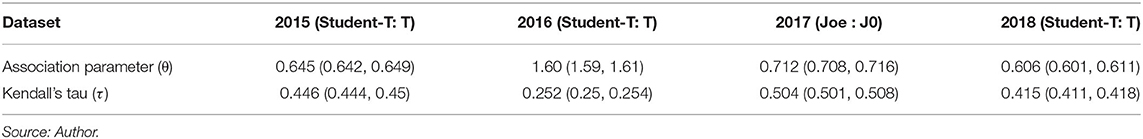
Table 4. Association parameters as confirmation of the presence of significant dependence.
The confirmation of the consistent presence of endogeneity due to reverse causality between affordability and housing tenure justifies the use of the joint binary regression modeling between housing tenure and housing affordability. The corresponding Kendall's tau results indicate that the association between housing tenure and affordability was strong for the 2018, 2017, and 2015 datasets, except for the 2016 dataset where the association was moderate.
The results above show that modeling housing affordability and housing tenure should always consider possible existence of joint dependency between the two variables. By applying the bivariate binary joint modeling in the presence on unobserved confounders (using appropriate copulas to model the errors), more errors are accounted for, and the final models produced are more reliable, as a basis for decision making.
The Coefficients
Tables A1–A4 in the Appendix A present the joint bivariate binary models with scaled coefficients. Apart from the household head age range above 95 years (for all the four datasets) and the Kazulu-Natal provincial variable for the 2016 dataset with respect to affordability, the rest of the parameters were significant at the 5% level for all datasets. The R-square values were not computed for the bivariate binary joint models because they do not hold any meaning for these non-linear bivariate joint binary (logit) models. The corresponding results for the univariate models were also generated and are in Tables B1A–B4B (Appendix B).
Factors That Most Significantly Influence Affordability and Home Ownership
The datasets were first scaled (using Equation 8) in order to obtain the coefficients in Tables A1–A4 (Appendix A). The research used the outcome equation (for housing tenure) instead of the treatment equation (for housing affordability) when comparing the rankings and when testing for the significance of differences between the coefficient values of both models (univariate and bivariate models).
Differences in Relative Influence of the Coefficients
The absolute values of the scaled coefficients for the bivariate joint models were then derived from the models and they were ranked according to their magnitude for each dataset. The procedure was also repeated and the absolute values of scaled coefficients for the univariate models were also generated. Table 5 shows the rankings representing the relative importance of the coefficients for both the bivariate joint binary model and the univariate model. The table also shows the differences in rankings and the mean rankings for all the four datasets. The smaller rank values indicate higher influence of a particular coefficient on the outcome (housing tenure):
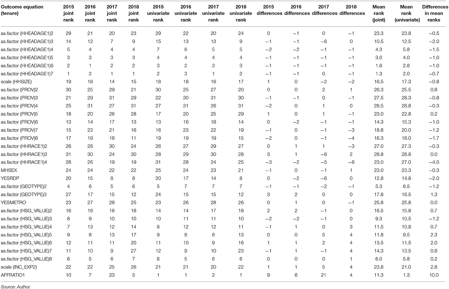
Table 5. Rankings for relative influence (severity) of the coefficients.
Differences in coefficient rankings between models: Because of the difference in nature of modeling between the joint bivariate binary model and the corresponding univariate model, there were significant differences between these models in the relative importance of the explanatory variables (with respect to housing tenure as the outcome). In this case, differences were highest in the affordability ratio (“AFFRATIO”), the household race [“(HHRACE1)4”], household income (“INC_EXP2”), house values between R 1,000,001 and 1,500,000, house values between R 1,500,001 and 2,000,000, subsidy beneficiary status (“YESRDP”), and household head age range from 40 to 49 years [“(HHEADAGE1)3”] in that order. The failure to take inter-dependency or reverse causality between housing affordability and housing tenure would mis-represent the relative importance of the housing affordability variable by an average of 10 ranking points for the 2015–2018 datasets (from the column of differences in mean ranks). However, further details show that the highest mis-representation of affordability was 21 ranking points in 2017 (2017 differences), while the lowest mis-representation was 4 ranking points in 2018 (2018 differences). Similar conclusions can be drawn for other variables.
Significance of Differences in the Coefficients
Equation (10) was used to evaluate the z-scores. Hypothesis testing was done for each coefficient with respect to each dataset. Table 6 shows the results. The symbol “E” indicates that there was significant evidence showing that the coefficient under consideration was the same for both models (Null hypothesis is true). The symbol “NE” indicates that the corresponding coefficient values in the two models were significantly not equal (Null hypothesis is false).
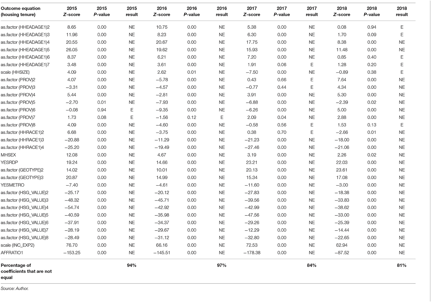
Table 6. Significance of the differences between the corresponding coefficient values.
The table shows further that the values of 94% of the coefficients used in the bivariate joint binary model for the 2015 dataset were significantly different from their corresponding values in the univariate model for the same dataset. The values for the 2016, 2017, and 2018 datasets were 97, 84, and 81%, respectively. The significant difference in most of the model coefficients shows that the severity of the influence of most of these coefficients would either be over-estimated or under-estimated, if a univariate model were to be used.
Other Observable Patterns of Influence
The odds ratios and probabilities discussed under this sub-section are conditional in nature. Table 5 shows that higher household head age ranges (above 49 years) exerted most influence on tenure. The higher age of a household head positively increased the probability of owner-occupancy, when the age was above 49 years. Other factors that exerted more influence on tenure were occupation of houses whose values were above R 3 million, location in a traditional geographical area, occupation of houses whose values were between R 250,001 and 500,000 (2015 and 2016 datasets), affordability ratio (2015, 2016, 2018 datasets), occupation of houses whose values were between R 500,001 and 1,000,000 (2015 dataset), occupation of houses whose values were between R 1,000,001 and 1,500,000 (2015 and 2016 datasets) and occupation of houses whose values were between R 2,000,001 and 3,000,000 (2016 and 2017 datasets). Other more detailed observable patterns in the 2018 dataset are shown in Table 7. Higher household head age ranges also exerted most influence on housing affordability. If other predictor variables were held constant, households with heads between ages of 49 and 65 years [(HHEADAGE1)4] were about 3.483 times or 248.3% more likely to have affordable housing compared to households whose heads were below 30 years (reference group). Their corresponding relative probability of having affordable housing was about 0.78. The odds ratios and probabilities when tenure was the response variable for the 2018 dataset of the same age category were 4.752 times or 375.2% more likely to be owner-occupiers (with probability of 0.826) compared to the age category below 30 years.
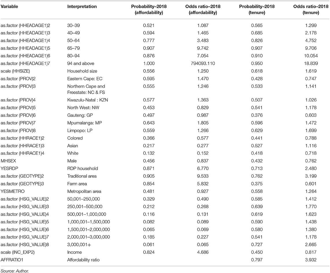
Table 7. Odds ratios and corresponding probabilities for the 2018 dataset.
Household size: Households with higher household sizes tended to have a higher likelihood of being affordable owner-occupiers. This is because the odds ratios for household sizes were greater than one (1) for both tenure and affordability as response variables. However, higher household sizes had a greater impact on tenure compared to affordability. Increasing household size may indicate a married couple or even more than one working adult in the household, which means more household income (as in the case of dual income households). On the other hand, larger household sizes may mean less desire for mobility when the need arises to transfer from one house to another when renting. This may lead such households to try and get a permanent home and avoid mobility inconveniences. The larger households will spend more on monthly rental amounts, due to demand for bigger space. If the rental amounts are significantly higher than the required monthly mortgage payments for home ownership, the households may opt to own their own home. On the other hand, small families which are new, and have just entered the workplace may usually not have the savings (say for down payment) to purchase a home. They may opt to rent while saving for a later purchase of their own residential property.
Provincial variations: The Western Cape province was taken to be the reference. Compared to the western cape province, the probability of owner-occupancy for the rest of the provinces was higher than the probability of renting, except for Gauteng province (probability was 0.376). The same pattern was also applicable when housing affordability was the response variable, with the exceptions being Gauteng (probability was 0.497) and the North-West provinces (probability was 0.453). Therefore, it was more likely for households to be renters and also face affordability problems in Gauteng province. This meant that a household located in Gauteng province was 0.603 times likely (or 39.7% less likely) to be an owner-occupier compared to a similar household in Western Cape.
Race: The black South African population group was taken as the reference. Compared to the black South African headed households, the probabilities of owner-occupancy for Asian, colored and white South African population groups (in that order) were lower than the probabilities for renting for these same groups. This trend also applied to housing affordability, with exception that the magnitude of these relatively lower probabilities was highest with colored, and lowest with white South Africans. This trend could be partly due to a number of reasons. The first reason could be due to effect of housing subsidies (such as RDP subsidies). Compared to other population groups, the black south African households consisted of majority of the South African Households and were the majority beneficiaries of housing subsidies, because of being part of the previously marginalized groups with respect to property rights ownership. Compared to its status when it is not a subsidy beneficiary, a household that was an RDP beneficiary had its likelihood of owner-occupancy increased almost 2.5 times or by 148%. The likelihood of having affordable tenure increased by 6.77 times (or by 577%). The second reason could be due to the effect of location of homes in traditional areas (GEOGTYPE 2). Compared to other population groups, majority of households living in traditional (rural) areas are black headed South African households. Table 7 shows that, other variables remaining constant, location of a household in a traditional area (compared to its location in urban areas) would approximately increase the likelihood of owner-occupancy by 3.2 times (or by 219.9%) and the likelihood of having affordable tenure by 9.5 times (or by 853.3%). Households located in farm areas are also less likely to face affordability problems but are more likely to be renters since the probability of owner-occupancy is >0.5 (probability is 0.375). Several Acts of Parliament have made provisions to improve living conditions, and provide secure and affordable tenure for workers who are farm dwellers (majority of whom are still black South Africans). These include the South African Extension of Security of Tenure Act (No. 62) of 1997 and the South African Housing Act (No. 107) of 1997 [55, 56]. Wherever farm subdivisions and transfer of ownership to workers in not possible, recommendations for renting through institutional subsidy programmes or some form of project-based rental housing development are proposed by the National Housing Code [24].
Property values: There was a tendency for households in South Africa to prefer owner-occupancy across all property price levels, when compared to the reference property price level (< R 50,000 level). The odds ratios were all greater than one (1), which meant there was a relatively higher probability of owner-occupancy compared to renting. However, the households were more likely to face affordability problems since the probabilities of having affordable tenure were all <0.5 across all property value levels. Since the housing affordability reduced as the property values increased, there were greater financial difficulties in acquiring higher priced homes. Higher household incomes, perhaps tended to favor affordable renting more than affordable owner-occupancy because higher-income households were more likely not to face affordability problems (probability of 0.824) but were less likely to be owner-occupiers (probability of 0.452).
Affordability ratios: Assuming other variables remained constant, the effect of the affordability ratio variable changing from zero (0) to one (1) would be to increase the likelihood of owner-occupancy 3.93 times (or by 293.2%). There were other impediments to owner-occupancy that were not captured by the model, such as the saving culture and actual household wealth which contribute toward sufficient household down-payment as a pre-requisite to obtaining a home loans.
Scenario without subsidies: The trend of older households being more likely to become owner-occupiers was true even though the housing RDP subsidies were not taken into consideration. A linear hypothesis analysis was run, having set the “YESRDP” variable to zero (0) instead of one (1), and the analysis was restricted to Eastern Cape province, for black South African household heads. Figure 1 shows the results.
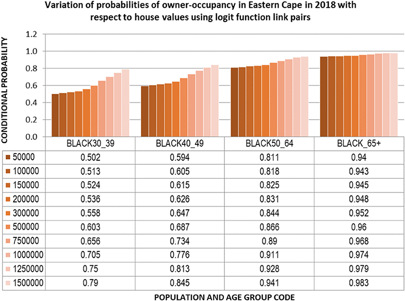
Figure 1. Variation of probabilities of owner-occupancy in Eastern Cape in 2018 (Source: Author).
The probability of owner-occupancy was lower for low-priced homes among younger households. Younger households tended to prefer ownership of residential property whose price was higher (indicating better quality). Thus, they opted to rent lower priced property, probably to save for future better home ownership. Younger households tend to be smaller in size or are even childless. Therefore, the inconvenience of movement from home to home while renting for the younger households may not be as great as the inconvenience experienced by older households, due to renting. The older households may, therefore, prefer staying in their own home, irrespective of its value or quality. This may explain why the graphs for older Black South African households are significantly higher than the rest of the other groups, with respect to lower priced homes. The graphs for these older households are also significantly less steep. This may indicate less motivation or demand to own new higher-priced homes, due to a reluctance to move or change homes. This is in agreement with the findings of Aliu [57], Clark [58], and Huang et al. [59] which show that age of the household and the presence of children in the household plays a significant role in household mobility.
Discussion
The most important finding for this research is that the bivariate joint binary regression modeling in the presence of endogenous treatment due to inter-dependence is more suitable for modeling of housing affordability and housing tenure, when compared to the respective univariate models. A consideration of presence of endogeneity due to reverse causality between housing tenure and housing affordability is therefore necessary when modeling within the South African context. The univariate and bivariate models were also compared. The differences in the modeling method has also revealed significant differences in rankings of the relative importance of some of the explanatory variables. There were also significant differences in most of the corresponding coefficient values when both models were compared. Since there is hardly any previous research that has attempted to jointly model housing affordability and tenure in this way, the significant difference in both the severity of the effects and the relative rankings of the influence of the individual explanatories should be borne in mind as a basis for distinct difference with previous findings, although the patterns with previous studies may appear similar.
This research also showed that higher (or older) household head-age category variables were the most significant in affecting housing affordability and housing tenure. The other variables that had high influence included house values, household location in traditional geographical areas, and affordability ratios. The large influence due to the older age of the household-head could be due to older South Africans having acquired more wealth (and hence having higher incomes) than younger ones. This wealth is a source of income for such people. Studies conducted among older citizens in other countries such as Australia confirm the fact that older citizens hold more income and wealth than younger ones to be true [60]. Owner-occupancy was heavily in favor of black-headed households because the South African black population group was the majority population group (80% of total population) in South Africa. In addition, since the black population group were among the previously marginalized groups, along with coloreds and Asians, they formed the majority of the beneficiaries of Government housing subsidies. Owner-occupancy in South African urban areas was also less likely compared to traditional areas and firms. Although the patterns are similar to some previous studies, the severity of the impact may differ due to differences in modeling techniques used.
Conclusions
This research has shown that there exists dependence between housing tenure and housing affordability. The bivariate binary joint model with endogenous treatment allows for dealing with this kind of problem much better than a univariate model. The research has also highlighted that both income and wealth have consistently been the most significant influencers of housing affordability and housing tenure in South Africa. Other important factors include property or house values, household location in traditional areas, and affordability ratios. Housing policy in South Africa should also be both space and time-specific owing to differing household lifecycle stages and profiles. It is important to investigate if there are significant improvements in the joint modeling of housing tenure and affordability, when non-linear additive predictors are used on individual cross section datasets. This is a further possible area of research.
Data Availability Statement
Publicly available datasets were analyzed in this study. The datasets can be found at: DOI: https://doi.org/10.25828/9tmn-fz97; DOI: https://doi.org/10.25828/6bvj-n342; DOI: https://doi.org/10.25828/ka3w-rg96; DOI: https://doi.org/10.25828/5b12-w270.
Ethics Statement
The studies involving human participants were reviewed and approved by the Faculty of Engineering Built Environment and Information Technology (EBEIT) Research Ethics Committee (Human), Nelson Mandela University. The data used was secondary data from national surveys. However, the patients/participants provided their written informed consent to participate in the national surveys.
Author Contributions
EK participated in writing most of the manuscript and analyzed the data. BB contributed to the concept and design of the work. He was also involved in drafting the work or revising it critically for important intellectual content. SM contributed to the acquisition of data for the work. He was also involved in drafting the work or revising it critically for important intellectual content. GC contributed substantially to the methodology development and execution. He was also involved in drafting this section or revising it critically for important intellectual content. All authors provided approval for publication of the content and agreed to be accountable for all aspects of the work in ensuring that questions related to the accuracy or integrity of any part of the work are appropriately investigated and resolved.
Conflict of Interest
The authors declare that the research was conducted in the absence of any commercial or financial relationships that could be construed as a potential conflict of interest.
Publisher's Note
All claims expressed in this article are solely those of the authors and do not necessarily represent those of their affiliated organizations, or those of the publisher, the editors and the reviewers. Any product that may be evaluated in this article, or claim that may be made by its manufacturer, is not guaranteed or endorsed by the publisher.
Acknowledgments
Acknowledgments go to Statistics South Africa for their support and cooperation and for making available the data on which this research has heavily depended.
Supplementary Material
The Supplementary Material for this article can be found online at: https://www.frontiersin.org/articles/10.3389/fams.2022.805524/full#supplementary-material
References
1. Coolen H, BoelHouwer P, Van Driel K. Values and goals as determinants of intended tenure choice. J Housing Built Environ. (2002) 17:215–36. doi: 10.1023/A:1020212400551
2. Carter S. Housing tenure choice and the dual income household. J Housing Econ. (2011) 20:159–70. doi: 10.1016/j.jhe.2011.06.002
3. Bazyl M. Factors influencing tenure choice in european countries. Central Euro J Econ Model Econ. (2009) 4:371–87.
4. Spalkova D, Spalek J. Housing tenure choice and housing expenditures in Czech republic. Rev Euro Stud. (2013) 6:23. doi: 10.5539/res.v6n1p23
5. Munford LA, Fichera E, Suttom M. Is owning your home good for your health? Evidence from exogenous variations in subsidies in England. Econ Human Biol. (2020) 39:100903. doi: 10.1016/j.ehb.2020.100903
6. Huang Y, Clark WAV. Housing tenure choice in transitional urban China: a multilevel analysis. Urban Stud. (2002) 39:7–32. doi: 10.1080/00420980220099041
7. Tandoh F, Tewari DD. The determinants of housing tenure choice. Evidence from micro data. Mediterranean J Soc Sci. (2013) 4:597. doi: 10.5901/mjss.2013.v4n13p597
8. Painter G. Tenure choice with sample selection: differences among alternative samples. J Hous Econ. (2000) 9:197–213. doi: 10.1006/jhec.2000.0266
9. Marra G, Papageorgiou G, Radice R. Estimation of a semiparametric recursive bivariate probit model with nonparametric mixing. Aust N Z J Stat. (2014) 55:341–2. doi: 10.1111/anzs.12043
10. Hanck C, Arnold M, Gerber A, Scmelzer M. Introduction to Econometrics With R. (2019). Available online at: https://www.econometrics-with-r.org/ITER.pdf (accessed May 20, 2020).
11. Guillermo BS, Maike H, Andreas G, Thomas K. Flexible instrumental variable distributional regression. J R Stat Soc. (2020) 183:1553–74. doi: 10.1111/rssa.12598
12. Marra G, Radice R. A joint regression modeling framework for analyzing bivariate binary data in R. Dependence Model. (2017) 5:268–94. doi: 10.1515/demo-2017-0016
13. Li J. Recent trends on housing affordability research: where are we up to? SSRN Electron J. (2015). doi: 10.2139/ssrn.2555439
14. Sun L. Housing Affordability in Chinese Cities. Working Paper WP20LS1. Lincoln Institute of Land Policy (2020). Available online at: https://www.lincolninst.edu/sites/default/files/pubfiles/sun_wp20ls1.pdf (accessed July 20, 2021).
15. Liao Y, Zhang J. Hukou status, housing tenure choice and wealth accumulation in urban China. China Econ Rev. (2020) 68:101638. doi: 10.1016/j.chieco.2021.101638
16. ECA-SA. Land Tenure Systems and Sustainable Development in Southern Africa. (2003). Available online at: https://sarpn.org/documents/d0000664/P672-ECA_Report.pdf (accessed June 13, 2021).
17. Kloppers HJ, Pienaar GJ. The historical context of land reform in South Africa and early policies. Potchefstroom Electronivc Law J. (2014) 17:676–706. doi: 10.4314/pelj.v17i2.03
18. Natives Land Act. c.27. (1913). Available online at: https://www.sahistory.org.za/archive/natives-land-act-act-no-27-1913 (accessed September 17, 2021).
19. Natives Urban Area Act. c.21. (1923). Available online at: https://disa.ukzn.ac.za/sites/default/files/pdf_files/leg19230614.028.020.021.pdf (accessed September 17, 2021).
20. Group Area Act. c.41. (1950). Available online at: https://blogs.loc.gov/law/files/2014/01/Group-Areas-Act-1950.pdf (accessed October 12, 2021).
21. Higgs B. The Group Areas Act its Effects. (1971). Available online at: http://www.aluka.org/action/showMetadata?doi=10.5555/AL.SFF.DOCUMENT.nuun1971_01 (accessed October 9, 2021).
22. South African Abolition of Racially Based Land Measures Act. c.108. (1991). Available online at: https://www.gov.za/sites/default/files/gcis_document/201409/a1081991.pdf (accessed September 17, 2021).
23. Huchzermeyer M, Harrison P, Charlton S, Klug N, Rubin M, Todes A. Urban land reform in South Africa: pointers for urban policy and planning. Town Regional Plann. (2019) 75:91–103. doi: 10.18820/2415-0495/trp75i1.10
24. DHS. National Housing Code, Vol. 1., Simplified Guide to the National Housing Code 2009. (2009). Pretoria: Government Printers. Available online at: http://www.dhs.gov.za/ (accessed May 12, 2020).
25. Cloete CE, editor. Property Finance in South Africa. 2nd ed. Pretoria: The South African Property Education Trust (2005).
26. Cloete CE, editor. Property Investment in South Africa. 2nd ed. Pretoria: The South African Property Education Trust (2005).
27. South African Sectional Titles Act. c.95. (1986). Available online at: https://www.gov.za/documents/sectional-titles-act-17-sep-1986-0000 (accessed September 17, 2021).
28. South African Time Shares control Act. c.75. (1983). Available online at: https://www.gov.za/sites/default/files/gcis_document/201504/act-75-1983.pdf (accessed September 10, 2021).
29. South African Upgrading of Land Tenure Rights Act. c.112. (1991). Available online at: https://www.gov.za/sites/default/files/gcis_document/201409/a1121991.pdf (accessed September 17, 2021).
30. Department for International Development. Land Issues Scoping Study: Communual Land Tenure Areas. (2003). Available online at: https://sarpn.org/documents/d0000646/P657-DFID.pdf (accessed June 10, 2021).
31. Department of Rural Development and Land Reform. Land Audit Report. Phase II: Private Land Ownership by Race, Gender and Nationality. (2017). Available online at: https://www.gov.za/sites/default/files/gcis_document/201802/landauditreport13feb2018.pdf (accessed September18, 2021).
32. STATSA. General Household Survey. (2018). Pretoria: Government Printers. Available online at: http://www.statssa.gov.za/publications/P0318/P03182018.pdf (accessed June 15, 2019).
33. Chakwizira J. Low-income housing backlogs and deficits “blues” in south africa. What solutions can a lean construction approach proffer? J Settlements Spatial Plann. (2019) 10:71–88. doi: 10.24193/JSSP.2019.2.01
34. STATSA. GDP: Quantifying SA's Economic Performance in 2020. (2021). Available online at: http://www.statssa.gov.za/?p=14074 (accessed March 29, 2021).
35. STATSA. General Household Survey, 2009. (2009). Pretoria: Government Printers. Available online at: http://www.statssa.gov.za/publications/P0318/P03182009.pdf (accessed June15, 2019).
36. Maclennan D, Williams R. Affordable Housing in Britain and America. York: Joseph Rowntree Foundation (1990).
37. Jewkess M, Delgadillo L. Weaknesses of housing affordability indices used by practitioners. J Financial Counsel Plann. (2010) 21:43–52. Available online at: https://ssrn.com/abstract=2222052
38. STATSA. General Household Survey, 2015. (2015). Pretoria: Government Printers. Available online at: http://www.statssa.gov.za/publications/P0318/P03182015.pdf (accessed June 15, 2019).
39. STATSA. General Household Survey, 2016. (2016). Pretoria: Government Printers. Available online at: http://www.statssa.gov.za/publications/P0318/P03182016.pdf (accessed June 15, 2019).
40. STATSA. General Household Survey, 2017. (2017). Pretoria: Government Printers. Available online at: http://www.statssa.gov.za/publications/P0318/P03182017.pdf (accessed June 15, 2019).
41. Dobson AJ, Barnett AG. An Introduction to Generalized Linear Models. 4th ed. Boca Raton, FL: Taylor & Francis Group, LLC (2018).
42. Wood SN. Low rank scale invariant tensor product smooths for generalized additive mixed models. Biometrics. (2006) 62:1025–36. doi: 10.1111/j.1541-0420.2006.00574.x
43. Radice R, Marra G, Wojtys M. Copula regression spline models for binary outcomes. Stat Comput. (2016) 26:981–95. doi: 10.1007/s11222-015-9581-6
44. Marra G. Package “GJRM”. (2021). Available online at: https://cran.r-project.org/web/packages/GJRM/GJRM.pdf (accessed March 12, 2021).
45. Hasebe T. Copula based maximum-likelihood estimation of sample-selection models. Stata J. (2013) 13:547–73. doi: 10.1177/1536867X1301300307
46. Marra G. Package “GJRM”. (2019). Available online at: https://cran.r-project.org/web/packages/GJRM/GJRM.pdf (accessed November 12, 2019).
47. Harrison E, DrakeT Ots R. Finalfit: Quickly Create Elegant Regression Results Tables and Plots When Modelling. R package version 1.0.2 (2020). Available online at: https://CRAN.R-project.org/package=finalfit (accessed November10, 2020).
48. Revelle W. An Introduction to the Psych Package: Part I: Data Entry and Data Description. (2020). Available online at: https://cran.r-project.org/web/packages/psych/vignettes/intro.pdf (accessed March 18, 2020).
49. Revelle W. An Introduction to the Psych Package: Part II: Scale Construction and Psychometrics. (2020). Available online at: https://pbil.univ-lyon1.fr/CRAN/web/packages/psych/vignettes/overview.pdf (accessed March 18, 2020).
50. Revelle W. How to: Part I: Use the Psych Package for Factor Analysis and Data Reduction. (2019). Available online at: https://cran.r-project.org/web/packages/psychTools/vignettes/factor.pdf (accessed March 18, 2020).
51. Gomes M, Radice R, Camarena-Brenes J, Marra G. Copula selection models for non-gaussian outcomes that are missing not at random. Stat Med. (2019) 38:480–96. doi: 10.1002/sim.7988
52. Gelman A. Scaling regression inputs by dividing by 2 standard deviations. Stat Med. (2008) 27:2865–73. doi: 10.1002/sim.3107
53. Clogg CC, Petkova E, Haritou A. Statistical methods for comparing regression coefficients between models. Am J Sociol. (1995) 100:1261–93. doi: 10.1086/230638
54. Tripathy JP. Secondary data analysis: ethical issues and challenges. Iran J Public Health. (2013) 42:1478–79.
55. South African Housing Act. c.107. (1997). Available online at: http://www.dhs.gov.za/sites/default/files/legislation/Housing_Act_107_of_1997.pdf (accessed September 17, 2021).
56. South African Extension of Security of Tenure Act. c.62. (1997). Available online at: https://www.gov.za/sites/default/files/gcis_document/201409/a62-97.pdf (accessed September 17, 2021).
57. Aliu IR. Unpacking the dynamics of intra-urban residential mobility in Nigerian cities: analysis of low-income families in Ojo Lagos. Cities. (2019) 85:63–79. doi: 10.1016/j.cities.2018.12.005
58. Clark WAV. Life course events and residential change: unpacking age effects on the probability of moving. Popul Res. (2013) 30:319–34. doi: 10.1007/s12546-013-9116-y
59. Huang X, Dijs M, Van Weesep J. Rural migrants' residential mobility: housing and locational outcomes of forced moves in China. Housing Theory Soc. (2018) 35:113–36. doi: 10.1080/14036096.2017.1329163
60. Australian Government Productivity Commission. Housing decisions of older Australians. (2015). Available Online at: https://www.pc.gov.au/research/completed/housing-decisions-older-australians/housing-decisions-older-australians.pdf (accessed April 12, 2021).
Keywords: housing affordability, endogeneity, housing tenure-of-choice, multicollinearity, association parameter
Citation: Kabundu E, Botha B, Mbanga S and Crafford G (2022) Application of Copulas to Improve the Modeling of Housing Tenure and Affordability. Front. Appl. Math. Stat. 8:805524. doi: 10.3389/fams.2022.805524
Received: 30 October 2021; Accepted: 11 February 2022;
Published: 15 March 2022.
Edited by:
Hien Duy Nguyen, The University of Queensland, AustraliaReviewed by:
Lochner Marais, University of the Free State, South AfricaBiljana Mileva Boshkoska, Institut Jožef Stefan (IJS), Slovenia
Copyright © 2022 Kabundu, Botha, Mbanga and Crafford. This is an open-access article distributed under the terms of the Creative Commons Attribution License (CC BY). The use, distribution or reproduction in other forums is permitted, provided the original author(s) and the copyright owner(s) are credited and that the original publication in this journal is cited, in accordance with accepted academic practice. No use, distribution or reproduction is permitted which does not comply with these terms.
*Correspondence: Emmanuel Kabundu, kabunduemmanuel@gmail.com