Reliable numerical treatment with Adams and BDF methods for plant virus propagation model by vector with impact of time lag and density
 Nabeela Anwar
 Shafaq Naz1
  Muhammad Shoaib
- 1Department of Mathematics, University of Gujrat, Gujrat, Pakistan
- 2Department of Mathematics, Commission on Science and Technology for Sustainable Development in the South University Islamabad, Attock, Pakistan
Plant disease incidence rate and impacts can be influenced by viral interactions amongst plant hosts. However, very few mathematical models aim to understand the viral dynamics within plants. In this study, we will analyze the dynamics of two models of virus transmission in plants to incorporate either a time lag or an exposed plant density into the system governed by ODEs. Plant virus propagation model by vector (PVPMV) divided the population into four classes: susceptible plants [S(t)], infectious plants [I(t)], susceptible vectors [X(t)], and infectious vectors [Y(t)]. The approximate solutions for classes S(t), I(t), X(t), and Y(t) are determined by the implementation of exhaustive scenarios with variation in the infection ratio of a susceptible plant by an infected vector, infection ratio of vectors by infected plants, plants' natural fatality rate, plants' increased fatality rate owing to illness, vectors' natural fatality rate, vector replenishment rate, and plants' proliferation rate, numerically by exploiting the knacks of the Adams method (ADM) and backward differentiation formula (BDF). Numerical results and graphical interpretations are portrayed for the analysis of the dynamical behavior of disease by means of variation in physical parameters utilized in the plant virus models.
Introduction
Plants provide food for humans and many other animals. They also provide medicines, clothing fibers, and are necessary for a healthy atmosphere. Plants, on the other hand, are susceptible to diseases, which are mostly triggered by viruses. The plant is frequently killed by these viruses. As a result, virus-related crop losses cost billions of dollars annually. Virus propagation is primarily carried out by a vector; insects which bite infectious plants become infected and subsequently infect susceptible plants. Seasonal behavior is common among insect vectors. They are most active throughout the summer and almost nearly dormant during the winter. Chemical pesticides are often employed as a control to battle vectors. Regrettably, these chemicals are not only overpriced, but they are also harmful to humans, animal life, as well as environment. Another option is to introduce a predator species, or just boost the population of one that already exists, to predate upon the insects as well as limit the virus's transmission. The vector population can be controlled with a combination of pesticides and predators. An effective mathematical model can be exploited to study the dynamics of pathogenic plant diseases. Indeed, mathematical analysis and numerical simulations are quite valuable in comprehending the dynamics of plant disease propagation and evaluating the impact of various disease control techniques.
Several mathematical models have been established to provide a detailed exposition of how to analyze, interpret, and forecast plant pathogenic farming epidemics as a mechanism for formulating and testing crop countermeasures and control measures [1–4]. A variety of epidemiology models based upon those used mostly in animal or human epidemiology have been created to assess the population ecosystem of viral infections [5–10]. The delay differential equations can be used to define relatively different formulations of epidemic proliferation. The application of delayed differential equations in epidemiological studies extends back to Van Der Plank's pioneering work [11], when these models were first proposed to represent plant diseases. The work of Van Der Plank seemed to have a limited impact on epidemic models, owing to the model hypotheses being particularly specific to plant pathology. However, a version of the Van Der Plank model has been shown to be well-suited to characterize human/animal diseases [12]. Stella et al. investigated the dynamics of the plant epidemic model and the presence and stability of distinct model equilibria. In the absence of delay, the Routh-Hurwitz criterion is employed to assess the stability of the disease free and epidemic equilibrium. In the existence of delay, the stability of epidemic equilibrium is also studied [13]. The bifurcation modulation of a fractional mosaic virus infectious disease model of Jatropha curcas with agricultural understanding and an executing delay was examined by Liu et al. Hopf bifurcation generated by the executing delay is explored for the unconstrained system by examining the corresponding characteristic equation [5]. Basir et al. developed a mathematical model that included multiple time delays as well as a Holling type-II functioning responses. The basic reproductive number and delays in time are used to determine the presence and stability of the equilibria. The delayed system's cost-effectiveness was assessed using the optimal control theory [14]. Ray et al. proposed a mathematical model to analyze the dynamics that included the incubation period as a time delay component for the vector-borne plant epidemic. The occurrence and stability of equilibrium have been investigated based on the reproduction number. Hopf bifurcation causes stability variations in the delaying and non-delaying systems [15]. Abraha et al. studied a mathematical model that included two time delays in agricultural pest management as well as the effect of farmer awareness. They assumed that the number of healthy parasites in the particular crop is proportionate to the growth of self-aware individuals. A saturation term is used to model the effects of awareness. The basic reproductive number, as well as time delays, are used to determine the presence and stability of the equilibrium. Whenever time delays reach the optimum values, stability transitions occur due to Hopf-bifurcation. The delayed system's cost-effectiveness was analyzed using adaptive control theory [16]. Phan et al. designed a system of differential equations including delay to represent the cell-to-cell propagation of infection by cereal and barley yellow dwarf pathogens throughout the plant. The model may capture a broad range of biologically pertinent phenomena through disease-free, epidemic, bilateral mortality equilibria, and a persistent periodical orbit by including a ratio-dependent incident function and logistic proliferation of healthy cells [17]. Blyuss et al. developed and analyzed a mathematical model for controlling the mosaic disease with natural microbiological biostimulants that, in addition to promoting plant development, also protect plants from infection via an RNA interference mechanism. They revealed how characteristics of biostimulants affect disease dynamics, and in particular, how they determine whether the mosaic disease is eliminated or preserved at a consistent level, by measuring the resilience of the system's equilibria [18]. Alemneh et al. introduced and assessed/analyzed an eco-epidemiological model of maize streak virus infection dynamics in order to evaluate the optimal strategy for preserving maize populations from the disease. To obtain an optimum controlling strategy, they applied the Pontryagin's maximum criterion to derive the Hamiltonian, control characterization, adjoint variables and the optimization system [19]. Amelia et al. presented a mathematical model of the yellow virus's spread in red chili plants, using the logistical function to predict the increase of insects as disease vectors. By calculating the dominating eigenvalue of the next generational matrix, we may determine the value of the fundamental reproduction number namely R0 of the model [20]. Kendig et al. investigated a mathematical model depicting the propagation of two viruses in a plant density, parameterized assuming empirically determined transmitting values, and discovered that nutrient pathogen communication could influence disease transmission. Thus, epidemic dynamics were regulated by interactions that affected propagation through viral density-independent pathways [21]. Shaw et al. compared the model based on individual and ordinary differential equation mathematical models to investigate the impact of insect vector living cycle and behavioral factors on the transmission of vector borne plant viruses. They discovered that evacuating virus infected species proved more effective than removing vector-infested species in terms of reducing infection [22]. The interactions within the plants, vectors and predators were described by Charpentier et al. using a system of ordinary differential equations. They used direct and indirect approaches to find the controls that minimize the optimization function subjected to population factors [23]. Jittamai et al. presented a mathematical framework to analyze the dynamics for Cassava Mosaic Virus, which is accelerated by both contaminated cuttings plantings and whitefly propagation. The model was used by the authors to determine the optimal cost-effective disease control strategy [24]. Charpentier recently presented two plant virus propagation models to illustrate the two perspectives of incorporating the delays. He numerically studied the models' stability [25].
Numerical techniques are generally employed in science as well as engineering to solve mathematical problems where exact solutions are difficult or impossible to obtain. Analytical solutions are only possible for a limited differential equation. For solving ordinary differential equations, there are a variety of analytical approaches. Even though, there are many ordinary differential equations (ODEs) whose solutions can be obtained in closed form using known analytical techniques, necessitating the progression and application of numerical methods in order to obtain the numerical solutions of a differential equation under the predefined initial condition. Various researchers have been intrigued by developing numerical techniques for solving initial value problems in ODEs in current years. Many researchers exploited various numerical techniques to approximate the solution of several mathematical models, yielding superior findings than a few of the existing ones in the literature, such as [26–30]. Recently research workers concentrated their efforts on numerically solving various mathematical models in the field of epidemiology such as COVID-19 [31], HIV model [32], tuberculosis transmission model [33], predator-prey mathematical model [34], mathematical model of cancer treatment [35]. Although the precision and stability of the aforementioned techniques are significant, they need a lot of memory and a long computation time. As a result, the numerical treatments for such approaches provide significant challenges that must be overcome in order to guarantee the precision and consistency of the solution. Therefore, ADM can be used to reliably confront one- and multi-dimensional stiff and non-stiff problems. The discrepancy between the predicted and corrected values might be used as one indicator of the error being made at each step. This gives a rather simple way to regulate the step size used in the integration. The widely used multistep ADM may approximate the solution of a first-order differential equation. In comparison to the equivalent-order Runge–Kutta method, these methods generally preserve reasonably good stability and accuracy properties while being more computationally efficient. When used with high order systems, this can significantly reduce computing time and effort. The most widely used techniques for treating stiff and non-stiff ODEs are implicit multistep techniques that utilize the BDF method. These methods were first used to confront a complex problem by Curtis and Hirschfelder [36]. Numerous implicit approaches have been created over time and are the subject of in-depth literature discussion; see [37–43]. To that end, the goal of this study is to apply the precise and stable ADM [44–48] and BDF methods to determine an initial value problem solution.
The paramount characteristics of this study are as follows: -
• The dynamics of two models of virus transmission in plants are investigated numerically to incorporate either a time lag or an exposed plant density into the system governed with non-linear delayed ODEs.
• The approximate solutions for classes S(t), I(t), X(t), and Y(t) are determined by the implementation of exhaustive scenarios with variation in the infection ratio of a susceptible plant by an infected vector, infection ratio of vectors by infected plants, plants' natural fatality rate, plants' increased fatality rate owing to illness, vectors' natural fatality rate, vector replenishment rate, and plants' proliferation rate.
• The approximate solutions of the non-linear plant virus propagation by a vector (PVPMV) are determined by exploiting the knacks of the Adams method (ADM) and backward differentiation formula (BDF) for sundry cases.
• Numerical and graphic interpretations of outcomes illustrate the significance/potential of these numerical methods as efficient, accurate, stable and viable computational procedures.
The remaining layout of the paper is as follows: Section Mathematical models presents mathematical models with relevant descriptions, Section Learning methodologies describes learning methodologies for the problem, Section Results and discussion provides results and discussion based on the numerical simulations, and Section Conclusions concludes with future research recommendations.
Mathematical models
Two plant virus models are presented here in this section. The mathematical model of plant virus propagation by a vector with a constant plant density is first presented. Second, a saturated and non-constant plant density plant virus propagation model is presented.
Plant virus propagation model by a vector: Model A
We investigate two models of vector-borne plant virus transmission. Both of these are basic, and the objective is to explore how different techniques of introducing the delay affect the outcomes. There are two plant densities in the first, model A: susceptible [S(t)], healthier and susceptible to infection, and infectious [I(t)], previously infected. Because we assume that plants may not recover, we should not have a recovered class. There are also two vector populations: susceptible [X(t)] and infectious [Y(t)]. This model is a simplified form of the models provided in [49, 50].
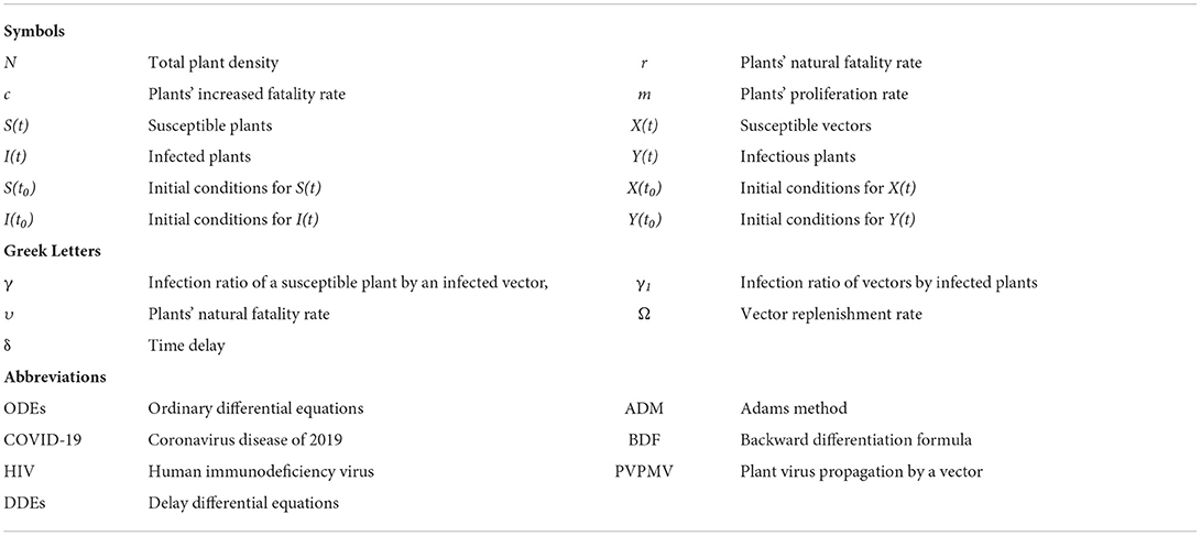
Model A assumes that: plants as well as vectors that are new to this field, are susceptible, and the overall plant density remains stable at N because a farmer may replace any dead plants with healthy new ones, that the interaction among both the vector as well as plant is a mass movement, that the viruses decapitate plants but not the vectors who do not contract the disease, and the disease cannot be recovered from either plants or vectors. The model's parameters are the γ infection ratio of a susceptible plant by an infected vector, γ1 infection ratio of vectors by infected plants, υ plants' natural fatality rate, c plants' increased fatality rate owing to illness, r vectors' natural fatality rate, and vector replenishment rate (according to birth or/and emigration).
Model A is represented by the system of ODEs as follows [25]:
There are two delays in virus transmission via a vector. One is being the time required for the virus to propagate throughout the plant after it has been infected. The other is the time required for the virus to propagate within the vector after it has been infected. Because the virus is not reproducing in the vector, the second is significantly smaller than the first. For the sake of simplicity, we'll assume that the second delay is zero.
We will incorporate the delays in two ways: the first is based on the premise that a susceptible needs the time delay to become infectious after coming into contact with an infectious [50, 51]. This is supposed to be model A1 [25]:
It would be possible to replace the exposed density [E(t)] with a delay-accounting density. After coming into contact with an infectious, a susceptible become exposed or dormant, unable to infect. The exposed becomes infectious at the rate η = 1/δ. Then the model A2 will be:
Epidemic models involving an exposed class are widely known for plant virus propagation [52, 53]. Models containing exposed densities have the advantage of not requiring the initial/staring conditions to be presented at an interval equal to the delay, as delay differential equations (DDEs) require.
Plant virus propagation model by vector: Model B
We construct a further plant virus propagation model which is based on the models presented in [54, 55], but revised to include healthy vectors and mass response interactions for the disease. It takes into account four different densities: susceptible plants [S(t)], infectious plants [I(t)], susceptible vectors [X(t)] and infectious vectors [Y(t)]. Because the plants grow in a logistical manner, the overall plant density does not remain constant. All emerging vectors are subject to susceptible, and their growth rate is continuously attributed to births as well as emigration. Plants are unable to recover and insects do not contract the disease, as it does in model A.
Model B, which propagates plant viruses is as follows [25]:
Here, m represents the plants' proliferation rate, N their maximum capacity of carrying, and γ the rate of infection of a susceptible plant by an infected vector, r represents the plants' natural fatality rate, and c represents the virus's additional fatality rate. Ω represents the rate at which susceptible vectors are recruited, γ1 represents the rate at which an infected plant infects a susceptible vector, and r represents the vectors' natural fatality rate.
We will incorporate the delay in two different ways, just like we did with model A. The first assumes that a susceptible takes the time delay to get infected after coming into contact with an infected [50, 51]. Then model B* may be expressed in the form [25]:
In the alternative version, we uphold [54, 55] in which the plant ceases being susceptible immediately after interaction with an infected insect, but it requires a delay period to become infected. Because the plant could die at any time, the surviving rate is directly proportional e−rδ, where r is the plant's fatality rate and δ is the delay. Then model B1 will be of the form [25]:
A susceptible plant is infected by an infected vector at time (t − δ) in model B*, as well as the susceptible plant becomes infective at time t. A susceptible plant is infected by an infected vector that takes t to infect in model B1, with e−rδ indicating the average rate of infectious susceptible who survived in time t.
Incorporating an exposed density [E(t)], as before, is an alternate with the same boon and bane. The model B2 with exposed class is as follows [25]:
Learning methodologies
Adams method
The Adams method (ADM) is a two-step procedure for solving an ODE [56–61]. First, to use an explicit approach, the predictive step determines a crude approximation of the target number. The corrector step streamlines the preceding approximation using a different mechanism, usually an implicit one.
The predictor-corrector technique, which is based on set of Equations (1)–(4), is represented as follows:
To obtain a two-step predictor solution for first equation of set (30) for the non-linear plant virus propagation model by vector, use the following expression:
We have the following two-step corrector equation after evaluating the first equation in the nonlinear plant virus propagation model by vector:
Backward differentiation method
The backward differentiation formula (BDF) is a collection of implicit approaches for solving ordinary differential equations numerically [62–64]. They are linear multi-step algorithms that use information from previously determined time points to approximating the derivative of a function for a particular function and time, improving the precision of the approximations. These techniques are particularly useful for solving stiff differential equations [65]. In 1952, Charles F. Curtiss and Joseph O. Hirschfelder introduced the methods for the first time.
Consider the initial value problem as:
BDF can be written in generic form as follows:
where the step size is denoted by h, g is being calculated for an unknown zn+l. BDF techniques are implicit and may require non-linear equations to be solved at each step. The coefficients cm as well as α are considered to obtain order l, which is the highest feasible order.
Table 1 [25] lists the default settings for the non-linear PVPMV parameters, while the nomenclature describes the parameters. These default settings utilizing in all of the scenarios of non-linear PVPMV.
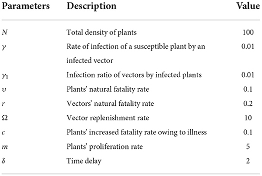
Table 1. Description and default parameters setting of for non-linear PVPMV [25].
Results and discussion
The approximate numerical outcomes for model A [25] having a constant plant density and model B [25] having a non-constant plant density are presented in this study. The ADM and BDF methods are used to explore the dynamics of first order non-linear plant virus propagation models by a vector for three variants of models A and B, respectively with inputs from [0, 30] and step size 0.1 for cases 1–5 of each distinct scenarios of nonlinear PVPMV. As shown in Table 2, the approximate solution for the variants of model A is obtained by creating different scenarios with cases 1–5 and varying the γ infection ratio of a susceptible plant by an infected vector, γ1 infection ratio of vectors by infected plants, υ plants' natural fatality rate, c plants' increased fatality rate owing to illness, r vectors' natural fatality rate, and Ω vector replenishment rate. Similarly, the approximate solution for the variants of model B is determined by using the impact of variation in m which represents the plants' proliferation rate, γ the rate of infection of a susceptible plant by an infected vector, r represents the plants' natural fatality rate, and c represents the disease's additional fatality rate. Ω represents the rate at which susceptible vectors are recruited, γ1 represents the rate at which an infected plant infects a susceptible vector, and r represents the vectors' natural fatality rate as shown in Table 2. Figure 1 depicts the working procedure of the designed approach for non-linear PVPMV.
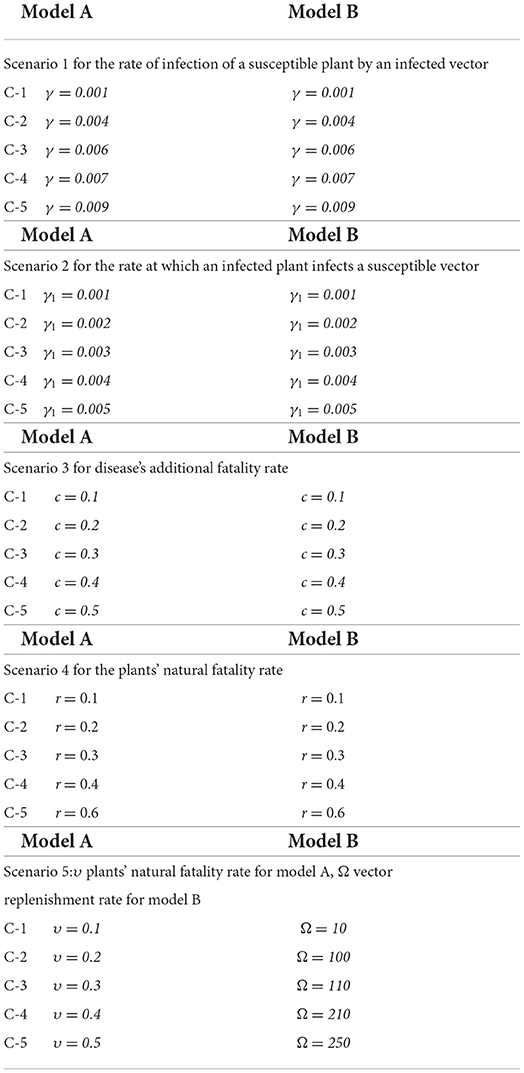
Table 2. Scenarios for model A and model B of non-linear PVPMV.
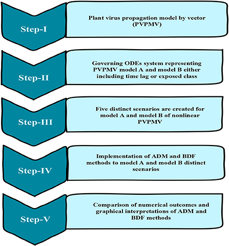
Figure 1. Working procedure of design approach for non-linear PVPMV.
Case study-I: Model A [25]
The three different models of plant virus propagation by a vector based on the system of ODEs without delay (model A), with delay (model A1), and without delay but including exposed class [E(t)] (model A2) as presented in Equations (1–4), (5–8), and (9–13) are numerically solved employing the ADM and BDF methods invoking he Mathematica routine with inputs [0, 30] and step size 0.1. Numerical outcomes and simulations are determined for five distinct scenarios of each model comprising cases 1–5 for non-linear PVPMV and selected random scenarios from each model for discussion. We first presented the dynamical behavior of S(t), I(t), X(t) and Y(t) classes of scenario 2 for model A of non-linear PVPMV. The numerical outcomes of non-linear PVPMV model A for case-1 of scenario 2 against the classes S(t), I(t), X(t) and Y(t) are listed in Table 3.

Table 3. Numerical outcomes of non-linear PVPMV model A for case-1 of scenario 2.
Figures 2A,B illustrate the dynamics of susceptible plants utilizing the ADM and BDF methods, respectively, for the variation in infection ratio of the vectors by infected plants, i.e., γ1 for model A. It has been discovered that increasing the value of γ1 causes the susceptible density of plants to drop. The impacts of infected plants are shown in Figures 3A,B for varied values of γ1. As can be seen from the graph, increasing the value of γ1 increases the density of infected plants. Figures 4A,B demonstrate that how the behavior of susceptible vectors changes as the value of γ1 changes. For higher values of γ1 there is an increase in the density of infected vectors. Figures 5A,B show the effects of infected vectors for various values of γ1. Increasing the value of γ1 increases the density of infected plants, as shown in the graphic.
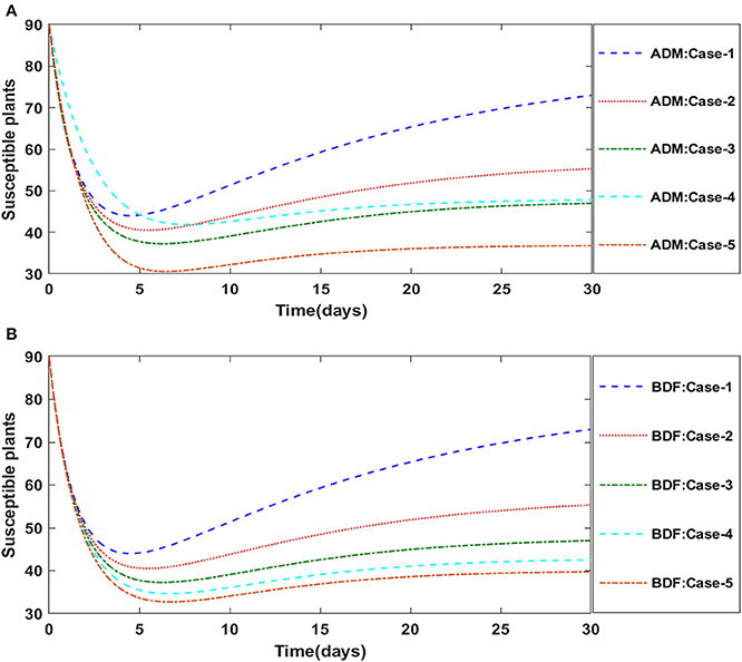
Figure 2. (A) Dynamics of susceptible plants for the varition in γ1 using ADM for model A. (B) Dynamics of susceptible plants for the varition in γ1 using BDF for model A.
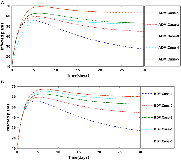
Figure 3. (A) Dynamics of infected plants for the varition in γ1 using ADM for model A. (B) Dynamics of infected plants for the varition in γ1 using BDF for model A.
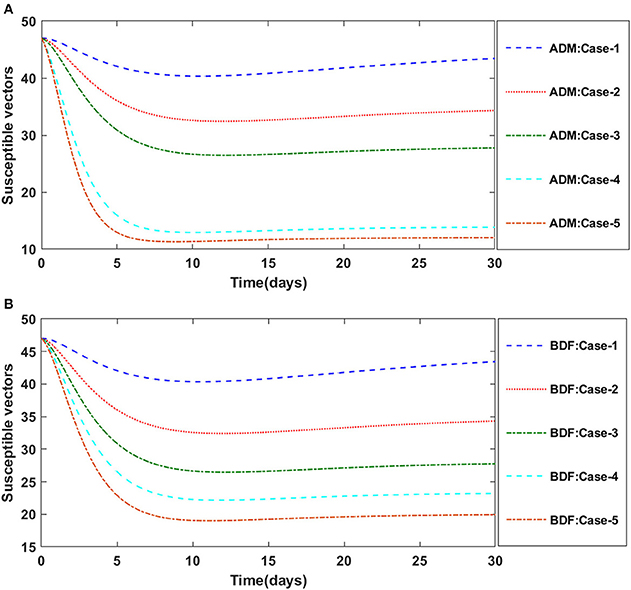
Figure 4. (A) Dynamics of susceptible vectors for the varition in γ1 using ADM for model A. (B) Dynamics of susceptible vectors for the varition in γ1 using BDF for model A.
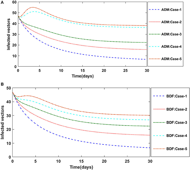
Figure 5. (A). Dynamics of infected vectors for the varition in γ1 using ADM for model A. (B) Dynamics of infected vectors for the varition in γ1 using BDF for model A.
The dynamics of plants' natural fatality rate i.e., υ is explored for all four classes S(t), I(t), X(t) and Y(t) using the strength of ADM and BDF methods for scenario 5 of the model A1. As seen in Figures 6A,B, raising the value of υ causes the density of susceptible plants to grow. The density of infected plants decreased as the value of υ increased, as seen in Figures 7A,B. Figures 8A,B show the effects of plants' natural mortality rate i.e., υ for class X(t) of model A1. As can be seen in the graphs, increasing the value of υ will increase the number of susceptible vectors. For class Y(t) of model A1, the influence of plants' natural fatality rate, i.e., υ is also computed. The rate of infected vectors reduces as the value of the infected vectors increases, as seen in Figures 9A,B. Table 4 shows the numerical outcomes of non-linear PVPMV model A1 for case-1 of scenario 5 against the classes S(t), I(t), X(t) and Y(t).
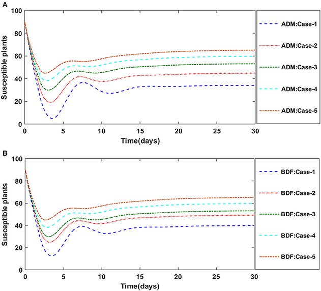
Figure 6. (A) Dynamics of susceptible plants for the varition in υ using ADM for model A1. (B) Dynamics of susceptible plants for the varition in υ using BDM for model A1.
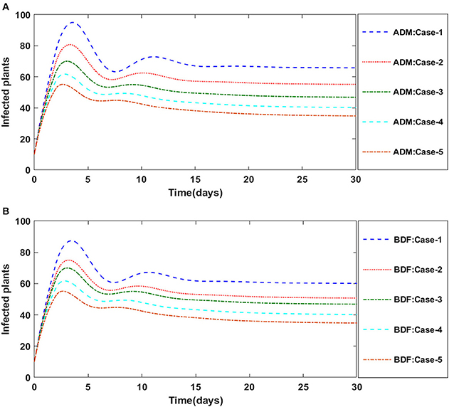
Figure 7. (A) Dynamics of infected plants for the varition in υ using ADM for model A1. (B) Dynamics of infected plants for the varition in υ using BDF for model A1.
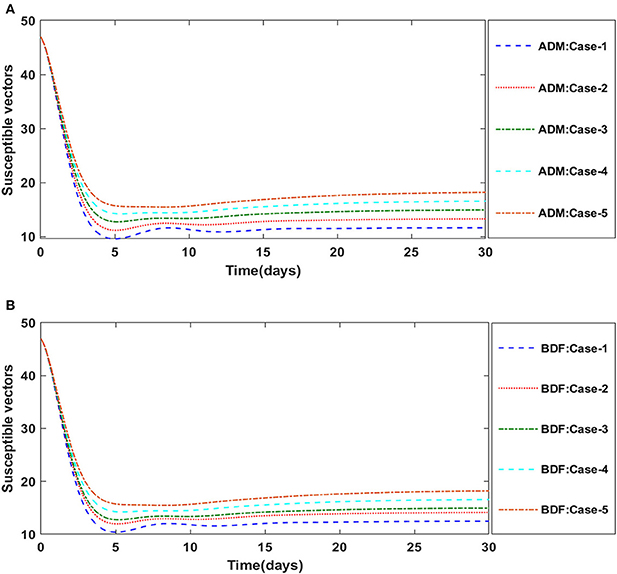
Figure 8. (A) Dynamics of infected plants for the varition in υ using ADM for model A1. (B) Dynamics of infected plants for the varition in υ using BDF for model A1.
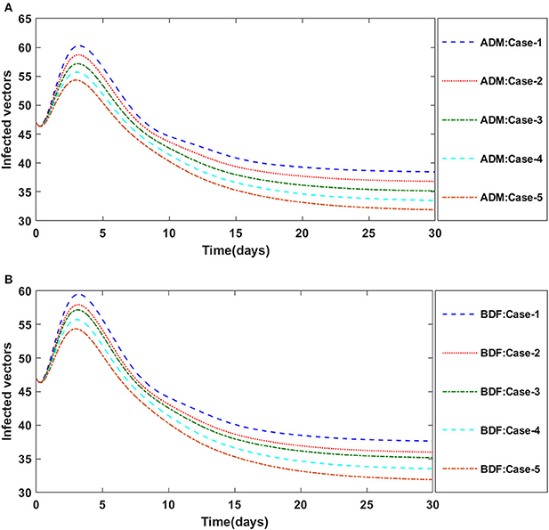
Figure 9. (A) Dynamics of susceptible vectors for the varition in r using ADM for model A1. (B) Dynamics of susceptible vectors for the varition in r using BDF for model A1.

Table 4. Numerical outcomes of non-linear PVPMV model A1 for case-1 of scenario 5.
Similarly, the dynamics for all four classes S(t), I(t), X(t) and Y(t)are analyzed by varying the infection ratio of a susceptible plant by an infected vector which is denoted by γ for scenario 1 of model A2 and graphical illustrations are presented in Figures 10–13, respectively. Numerical outcomes classes S(t), I(t), X(t) and Y(t) in model A2 for case-1 of scenario 1 are computed and provided in Table 5. Figures 10A,B depict the influence of the infection ratio of a susceptible plant by an infected vector on susceptible plants using the ADM and BDM methods, respectively. It is permissible to observe that when the value of γ rises, the density of susceptible plants decreases. Figures 11A,B describe the effects of the infection ratio of a susceptible plant by an infected vector on infected plants. One may observe that the density of infected plants increased in correlation with the value of γ. Figures 12A,B illustrate progressive increase in the density of susceptible vectors as the value of γ increases, whereas Figures 13A,B demonstrate the opposing behavior in the case of infected vectors.
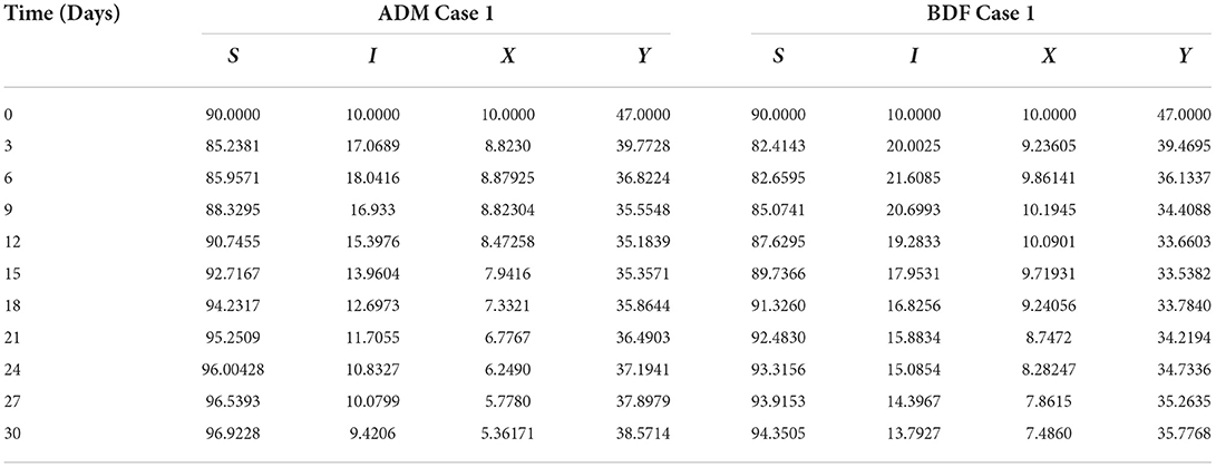
Table 5. Numerical outcomes of non-linear PVPMV model A2 for case-1 of scenario 1.
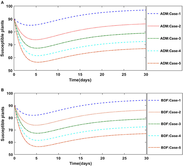
Figure 10. (A) Dynamics of susceptible plants for the varition in γ using ADM for model A2. (B) Dynamics of susceptible plants for the varition in γ using BDF for model A2.
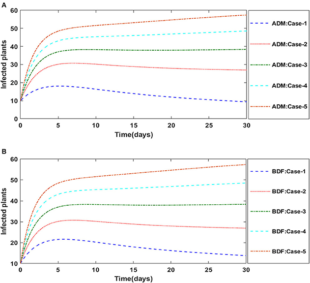
Figure 11. (A) Dynamics of infected plants for the varition in γ using ADM for model A2. (B) Dynamics of infected plants for the varition in γ using BDF for model A2.
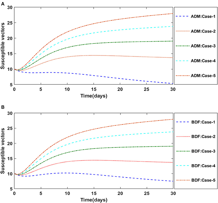
Figure 12. (A) Dynamics of susceptible vectors for the varition in γ using ADM for model A2. (B) Dynamics of susceptible vectors for the varition in γ using ADM for model A2.
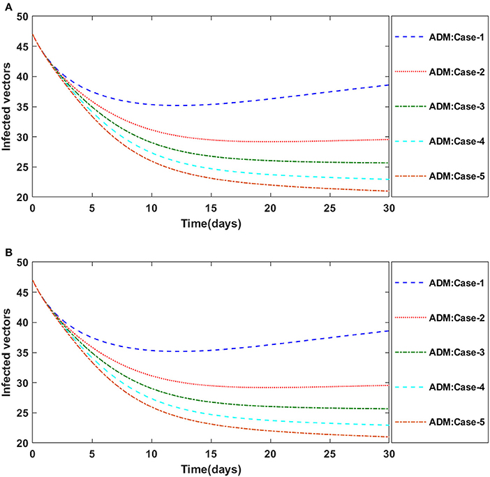
Figure 13. (A) Dynamics of infected vectors for the varition in γ using ADM for model A2. (B) Dynamics of infected vectors for the varition in γ using ADM for model A2.
Case study-II: Model B
The three segregated models of plant virus transmission by a vector, as described in Equations (14–17), (21–24), and (25–29), are numerically solved employing the ADM and BDF methods invoking the Mathematica routine. We construct five distinct scenarios incorporating cases 1–5 for non-linear PVPMV and chosen random scenarios from each model are used to determine numerical outcomes and simulations. For model B of non-linear PVPMV. We first described the dynamical behavior of the S(t), I(t), X(t), and Y(t) classes in scenario 3 for the variation in disease's additional fatality rate i.e., c. for model B. For all four classes S(t), I(t), X(t), and Y(t) numerical outcomes are determined and provided in Table 6 for case-1 of scenario 3 of model B. Figures 14A,B illustrate the dynamics of susceptible plants using the ADM and BDF methods for the variability in the disease's additional fatality rate i.e., c. It has been discovered that as the value of c is elevated, the susceptible density of plants increases. The impact of disease's additional fatality rate i.e., c on infected plants can be seen in Figures 15A,B. It is clear from Figures that increasing the value of c will result in reduction the density of infected plants. Figures 16A,B demonstrate the behavior of susceptible vectors for the variation in disease's additional fatality rate of model B. One may see that the density of susceptible vectors will increase as the value of c is increased. The influence of disease's additional fatality rate on infected vectors is presented in Figures 17A,B. It is observed from Figures that increasing the value of c causes the density of infected vectors to decrease.
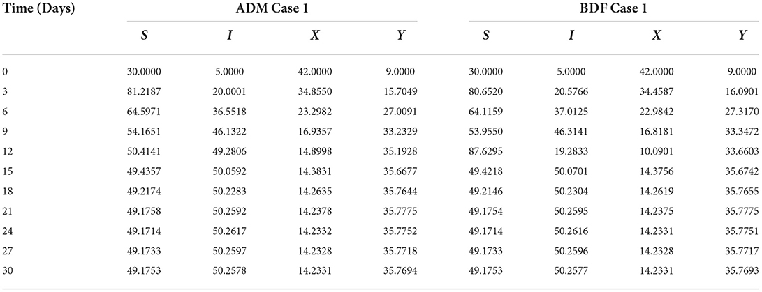
Table 6. Numerical outcomes of nonlinear PVPMV model B for case-1 of scenario 3.
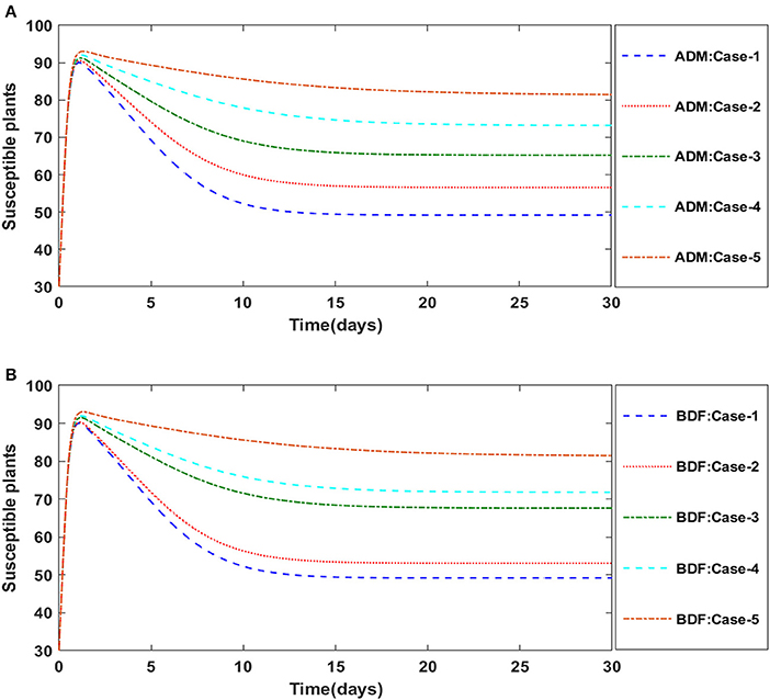
Figure 14. (A) Dynamics of susceptible plants for the varition in c using ADM for model B. (B) Dynamics of susceptible plants for the varition in c using BDF for model B.
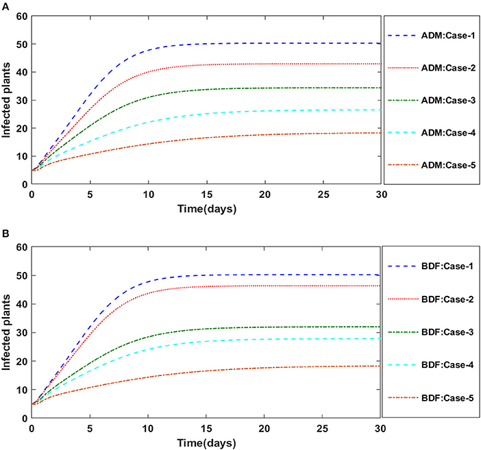
Figure 15. (A) Dynamics of infected plants for the varition in d using ADM for model B. (B) Dynamics of infected plants for the varition in d using BDF for model B.
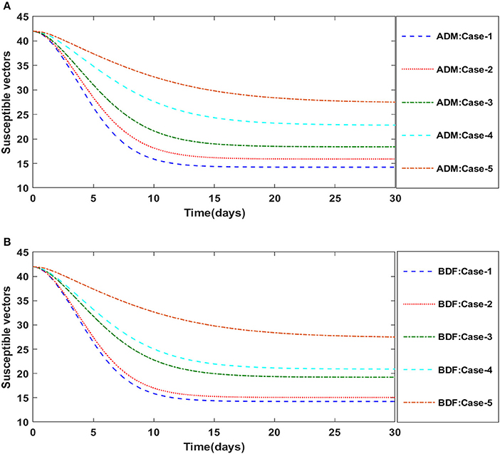
Figure 16. (A) Dynamics of susceptible vectors for the varition in d using ADM for model B. (B) Dynamics of susceptible vectors for the varition in d using BDF for model B.
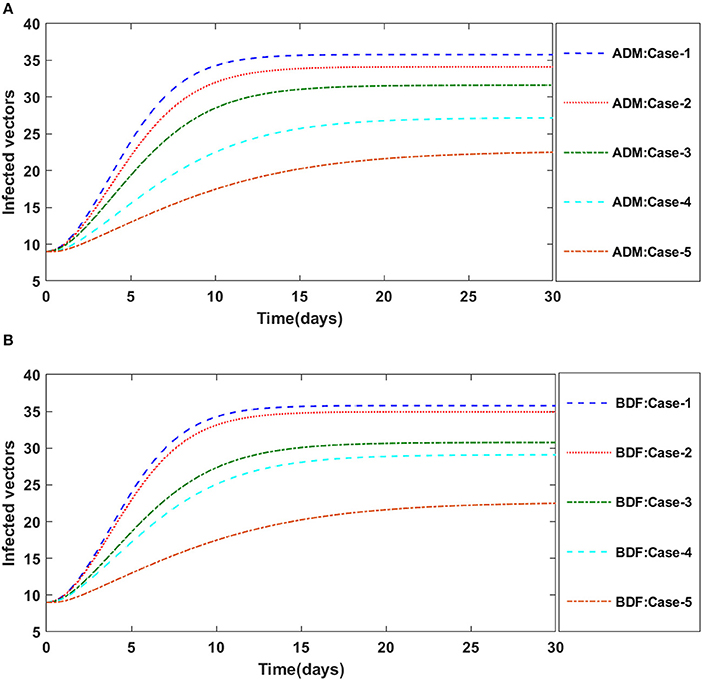
Figure 17. (A) Dynamics of infected vectors for the varition in d using ADM for model B. (B) Dynamics of infected vectors for the varition in d using BDF for model B.
Secondly, the dynamics of susceptible vectors' recruited rate i.e., Ω is investigated for all four classes S(t), I(t), X(t), and Y(t) utilizing the strength of ADM and BDF methods for scenario 5 of the model B1 and numerical outcomes of all four classes S(t), I(t), X(t), and Y(t) for the case-1 of scenario 5 is listed in Table 7. Figures 18A,B portrayed the behavior of susceptible plants density for the different values of Ω, and it is noticed that the number of susceptible plants decreases for the higher values of Ω. Figures 19A,B illustrated that as the value of Ω increases, the number of infected plants goes up. The dynmics of susceptible vectors for the variation in vectors' recruited rate i.e., c are presented in Figures 20A,B. One may witness that in Figures 20A,B the density of susceptible vectors goes in continous behavior for the first two cases and next three cases vectors density increased in the range of 0 to 10 days then steadily decreased and shows their steady behavior for next 20–30 days. As a result, for higher values of Ω, the density of susceptible vectors increases. Figures 21A,B portrayed the impact of susceptible vectors' recruited rate on infected vectors for model B1. The infected vectors show a steady behavior for the first two cases, also a steady behavior for the next three cases in 0–5 days, and then a gradual increase in 5–30 days, as shown in Figures 21A,B.
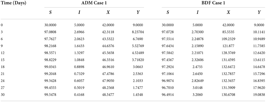
Table 7. Numerical outcomes of non-linear PVPMV model B1 for case-1 of scenario 5.
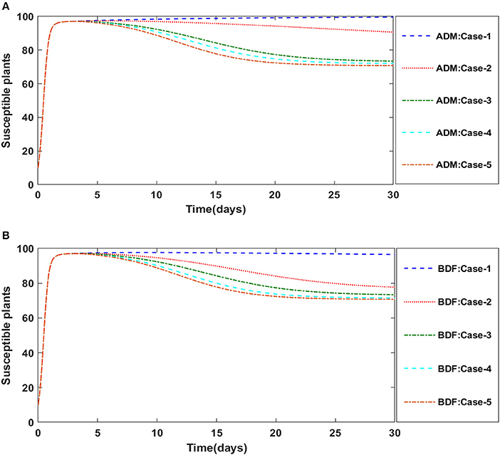
Figure 18. (A) Dynamics of susceptible plants for the varition in Ω using ADM for model B1. (B) Dynamics of susceptible plants for the varition in Ω using BDF for model B1.
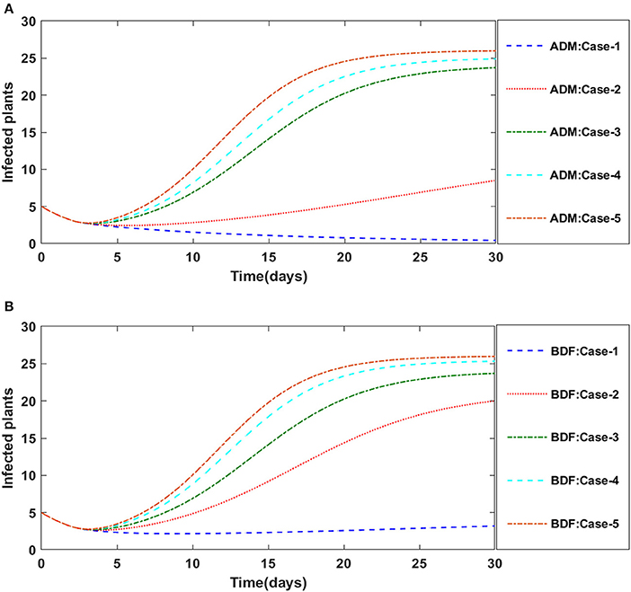
Figure 19. (A) Dynamics of infected plants for the varition in Ω using ADM for model B1. (B) Dynamics of infected plants for the varition in Ω using BDF for model B1.
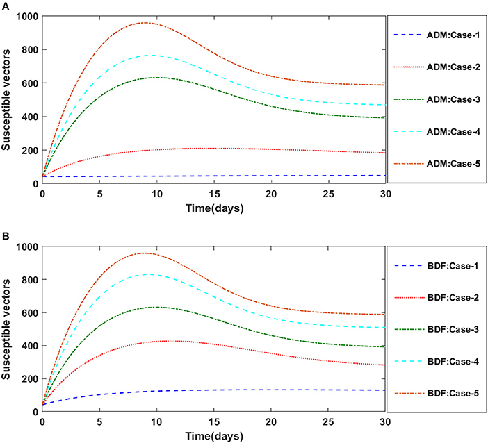
Figure 20. (A) Dynamics of susceptible vectors for the varition in Ω using ADM for model B1. (B) Dynamics of susceptible vectors for the varition in Ω using BDF for model B1.
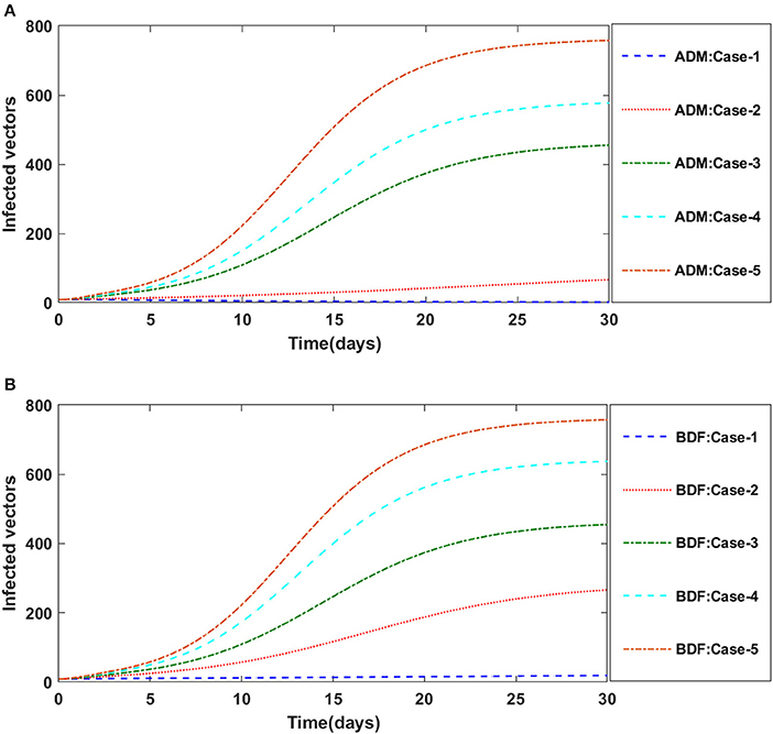
Figure 21. (A) Dynamics of infected vectors for the varition in Ω using ADM for model B1. (B) Dynamics of infected vectors for the varition in Ω using BDF for model B1.
Finally, the dynamics of vectors' natural fatality rate i.e., r is investigated for all four classes S(t), I(t), X(t), and Y(t) utilizing the strength of ADM and BDF methods for scenario 4 of the model B2. The respective numerical outcomes for case-1 of scenario 4 is provided in Table 8. The impact of vectors' natural fatality rate on susceptible plants is presented in Figures 22A,B As observed in graphical representation, the density of susceptible plants increased up to 90, then decreased between 3 and 10 days before returning to their steady state behavior. Also, the density of susceptible plants increased for the higher value of r as shown in Figures 22A,B, while the infected plants depicted reverse behavior as shown in Figures 23A,B. The influence of vectors' natural fatality rate r on susceptible vectors can be observed in Figures 24A,B for model B2. The number of susceptible vectors appears to decrease as the value of r increases. Similarly, the dynamics of infected vectors is portrayed in Figures 25A,B utilizing the ADM and BDF fro model B2, respectively. The number of infected vectors dropped as the natural fatality rate r of the vectors increased in model B2.
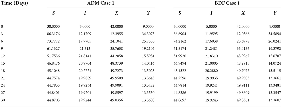
Table 8. Numerical outcomes of nonlinear PVPMV model B2 for case-1 of scenario 4.
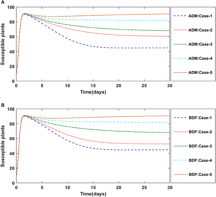
Figure 22. (A) Dynamics of susceptible plants for the varition in r using ADM for model B2. (B) Dynamics of susceptible plants for the varition in r using BDF for model B2.
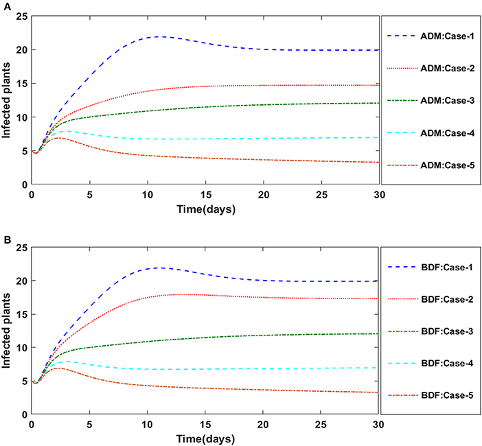
Figure 23. (A) Dynamics of infected plants for the varition in r using ADM for model B2. (B) Dynamics of infected plants for the varition in r using BDF for model B2.
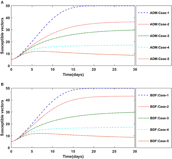
Figure 24. (A) Dynamics of susceptible vectors for the varition in r using ADM for model B2. (B) Dynamics of susceptible vectors for the varition in r using BDF for model B2.
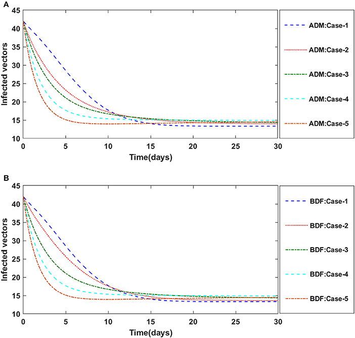
Figure 25. (A) Dynamics of infected vectors for the varition in r using ADM for model B2. (B) Dynamics of infected vectors for the varition in r using BDF for model B2.
Conclusions
In this paper, we analyzed the dynamics of two models of virus transmission in plants to incorporate either a time lag or an exposed plant density into the system governed with non-linear delayed ODEs. The presented models may effectively predict susceptible plants [S(t)], infected plants [I(t)], susceptible vectors [X(t)], and infectious vectors [Y(t)]. Numerical analysis of the plant virus propagation model by a vector (PVPMV) is conducted through exhaustive scenarios with variation in different parameters used in the models. The approximate solution of the non-linear PVPMV is determined by exploiting the knacks of the Adams method (ADM) and backward differentiation formula (BDF) method We found delayed models to have a greater degree of realism since they account for the time between contact and infection. Processes are affected by delay and mathematically delay influences the dynamics along with stability. Moreover, the presented study proved to be extremely useful in controlling the plant outbreak in the subsequent seasons.
The dynamics of non-linear fluid dynamic models may be investigated in the future utilizing the strength of Adams predictor corrector method and BDF method [66–69].
Data availability statement
The original contributions presented in the study are included in the article/supplementary material, further inquiries can be directed to the corresponding author/s.
Author contributions
NA prepared methodology, results, and discussion. SN prepared introduction. MS prepared abstract and conclusion. All authors contributed to the article and approved the submitted version.
Conflict of interest
The authors declare that the research was conducted in the absence of any commercial or financial relationships that could be construed as a potential conflict of interest.
Publisher's note
All claims expressed in this article are solely those of the authors and do not necessarily represent those of their affiliated organizations, or those of the publisher, the editors and the reviewers. Any product that may be evaluated in this article, or claim that may be made by its manufacturer, is not guaranteed or endorsed by the publisher.
References
1. Rossi V, Sperandio G, Caffi T, Simonetto A, Gilioli G. Critical success factors for the adoption of decision tools in IPM. Agronomy. (2019) 9:710. doi: 10.3390/agronomy9110710
2. Shelton AM, Long SJ, Walker AS, Bolton M, Collins HL, Revuelta L, et al. First field release of a genetically engineered, self-limiting agricultural pest insect: evaluating its potential for future crop protection. Front Bioeng Biotechnol. (2020) 7:482. doi: 10.3389/fbioe.2019.00482
3. Chowdhury J, Al Basir F, Takeuchi Y, Ghosh M, Roy K. A mathematical model for pest management in Jatropha curcas with integrated pesticides-an optimal control approach. Ecol Complex. (2019) 37:24–31. doi: 10.1016/j.ecocom.2018.12.004
4. Pratiwi NP, Aldila D, Handari BD, Simorangkir GM. November. A mathematical model to control Mosaic disease of Jatropha curcas with insecticide and nutrition intervention. AIP Conf Proc. (2020) 2296:020096. doi: 10.1063/5.0030426
5. Liu S, Huang M, Wang J. Bifurcation control of a delayed fractional mosaic disease model for jatropha curcas with farming awareness. Complexity. (2020) 2020:2380451. doi: 10.1155/2020/2380451
6. Al Basir F, Ray S. Impact of farming awareness based roguing, insecticide spraying and optimal control on the dynamics of mosaic disease. Ricerche Matematica. (2020) 69:393–412. doi: 10.1007/s11587-020-00522-8
7. Wei X, Wang L, Jia Q, Xiao J, Zhu G. Assessing different interventions against Avian Influenza A (H7N9) infection by an epidemiological model. One Health. (2021) 13:100312. doi: 10.1016/j.onehlt.2021.100312
8. Ratchford, C. Multi-scale and multi-group modeling techniques applied to Cholera and COVID-19 (Dissertation). The University of Tennessee at Chattanooga, Chattanooga, TN, United States. (2021).
9. Kwasi-Do Ohene Opoku N, Afriyie C. The role of control measures and the environment in the transmission dynamics of cholera. Abstract Appl Anal. (2020) 2020:2485979. doi: 10.1155/2020/2485979
10. Moore SE, Okyere E. Controlling the transmission dynamics of COVID-19. arXiv[Preprint].arXiv:2004.00443. (2020).
11. Van der Plank JE. Dynamics of epidemics of plant disease: Population bursts of fungi, bacteria, or viruses in field and forest make an interesting dynamical study. Science. (1965) 147:120–4. doi: 10.1126/science.147.3654.120
12. Noviello A, Romeo F, De Luca R. Time evolution of non-lethal infectious diseases: a semi-continuous approach. Eur Phys J B Cond Matter Complex Syst. (2006) 50:505–11. doi: 10.1140/epjb/e2006-00163-4
13. Stella IR, Srivastav AK, Ghosh M. May. Modeling and analysis of vector-borne plant disease with two delays. J Phys Conf Series. (2021) 1850:012125. doi: 10.1088/1742-6596/1850/1/012125
14. Al Basir F. A multi-delay model for pest control with awareness induced interventions—Hopf bifurcation and optimal control analysis. Int J Biomath. (2020) 13:2050047. doi: 10.1142/S1793524520500473
15. Ray S, Al Basir F. Impact of incubation delay in plant–vector interaction. Math Comput Simul. (2020) 170:16–31. doi: 10.1016/j.matcom.2019.09.001
16. Abraha T, Al Basir F, Obsu LL, Torres DF. Pest control using farming awareness: Impact of time delays and optimal use of biopesticides. Chaos Solitons Fractals. (2021) 146:110869. doi: 10.1016/j.chaos.2021.110869
17. Phan T, Pell B, Kendig AE, Borer ET, Kuang Y. Rich dynamics of a simple delay host-pathogen model of cell-to-cell infection for plant virus. Discrete Continuous Dyn Syst B. (2021) 26:515. doi: 10.3934/dcdsb.2020261
18. Blyuss KB, Al Basir F, Tsygankova VA, Biliavska LO, Iutynska GO, Kyrychko SN, et al. Control of mosaic disease using microbial biostimulants: insights from mathematical modelling. Ricerche Matematica. (2020) 69:437–55. doi: 10.1007/s11587-020-00508-6
19. Alemneh HT, Kassa AS, Godana AA. An optimal control model with cost effectiveness analysis of Maize streak virus disease in maize plant. Infect Dis Modell. (2021) 6:169–82. doi: 10.1016/j.idm.2020.12.001
20. Amelia R, Anggriani N, Istifadah N, Supriatna AK. Dynamic analysis of mathematical model of the spread of yellow virus in red chili plants through insect vectors with logistical functions. AIP Conf Proc. (2020) 2264:040006. doi: 10.1063/5.0023572
21. Kendig AE, Borer ET, Boak EN, Picard TC, Seabloom EW. Host nutrition mediates interactions between plant viruses, altering transmission and predicted disease spread. Ecology. (2020) 101:e03155. doi: 10.1002/ecy.3155
22. Shaw AK, Igoe M, Power AG, Bosque-Pérez NA, Peace A. Modeling approach influences dynamics of a vector-borne pathogen system. Bull Math Biol. (2019) 81:2011–28. doi: 10.1007/s11538-019-00595-z
23. Chen-Charpentier B, Jackson M. Optimal control of plant virus propagation. Math Methods Appl Sci. (2020) 43:8147–57. doi: 10.1002/mma.6244
24. Jittamai P, Chanlawong N, Atisattapong W, Anlamlert W, Buensanteai N. Reproduction number and sensitivity analysis of cassava mosaic disease spread for policy design. Math Biosci Eng. (2021) 18:5069–93. doi: 10.3934/mbe.2021258
25. Chen-Charpentier B. Delays in plant virus models and their stability. Mathematics. (2022) 10:603. doi: 10.3390/math10040603
26. Zaky MA. Existence, uniqueness and numerical analysis of solutions of tempered fractional boundary value problems. Appl Num Math. (2019) 145:429–57. doi: 10.1016/j.apnum.2019.05.008
27. Banu MS, Raju I, Mondal S. A comparative study on classical fourth order and butcher sixth order Runge-Kutta methods with initial and boundary value problems. Int J Mat Math Sci. (2021) 3:8–21. doi: 10.34104/ijmms.021.08021
28. Hossen M, Ahmed Z, Kabir R, Hossan Z. A comparative investigation on numerical solution of initial value problem by using modified Euler method and Runge Kutta method. ISOR J Math. (2019) 15:2278–5728. doi: 10.9790/5728-1504034045
29. Kafle J, Thakur BK, Acharya G. Formulative visualization of numerical methods for solving non-linear ordinary differential equations. Nepal J Math Sci. (2021) 2:79–88. doi: 10.3126/njmathsci.v2i2.40126
30. Koroche KA. Numerical solution of first order ordinary differential equation by using Runge-Kutta method. Int J Syst Sci Appl Math. (2021) 6:1–8. doi: 10.11648/j.ijssam.20210601.11
31. Olivares A, Staffetti E. Uncertainty quantification of a mathematical model of COVID-19 transmission dynamics with mass vaccination strategy. Chaos Solitons Fractals. (2021) 146:110895. doi: 10.1016/j.chaos.2021.110895
32. Campos C, Silva CJ, Torres DF. Numerical optimal control of HIV transmission in Octave/MATLAB. Math Comput Applic. (2019) 25:1. doi: 10.3390/mca25010001
33. Fatmawati MAK, Bonyah E, Hammouch Z, Shaiful EM. A mathematical model of tuberculosis (TB) transmission with children and adults groups: a fractional model. Aims Math. (2020) 5:2813–42. doi: 10.3934/math.2020181
34. Bürger R, Chowell G, Gavilán E, Mulet P, Villada LM. Numerical solution of a spatio-temporal predator-prey model with infected prey. Math Biosci Eng. (2019) 16:438–73. doi: 10.3934/mbe.2019021
35. Sweilam NH, Al-Mekhlafi SM, Assiri T, Atangana A. Optimal control for cancer treatment mathematical model using Atangana–Baleanu–Caputo fractional derivative. Adv Diff Equat. (2020) 2020:1–21. doi: 10.1186/s13662-020-02793-9
36. Curtiss CF, Hirschfelder JO. Integration of stiff equations. Proc Natl Acad Sci. (1952) 38:235–43. doi: 10.1073/pnas.38.3.235
37. Ebadi M, Gokhale MY. Hybrid BDF methods for the numerical solutions of ordinary differential equations. Num Alg. (2010) 55:1–17. doi: 10.1007/s11075-009-9354-4
38. Cash J. Efficient numerical methods for the solution of stiff initial-value problems and differential algebraic equations. Proc R Soc Lond Ser A Math Phys Eng Sci. (2003) 459:797–815. doi: 10.1098/rspa.2003.1130
39. Ogunrinde RB, Fadugba SE, Okunlola JT. On some numerical methods for solving initial value problems in ordinary differential equations. On Some Numerical Methods for Solving Initial Value Problems in Ordinary Differential Equations. (2012).
40. Lapidus L, Schiesser WE. Numerical Methods for Differential Systems: Recent Developments in Algorithms, Software, and Applications. (1976). doi: 10.1016/C2013-0-11041-0
41. Shampine LF. Numerical Solution of Ordinary Differential Equations. New York, NY: Routledge (2018). doi: 10.1201/9780203745328
42. Nasarudin AA, Ibrahim ZB, Rosali H. On the integration of stiff ODEs using block backward differentiation formulas of order six. Symmetry. (2020) 12:952. doi: 10.3390/sym12060952
43. Samson O, Victor JK. An application of second derivative ten step blended block linear multistep methods for the solutions of the holling tanner model and van der pol equations. Covenant J Phys Life Sci. (2019) 7:1–11. doi: 10.20370/s8gx-ft87
44. Qin G, Lou W, Wang H, Wu Z. High Efficiency and Precision Approach to Milling Stability Prediction Based on Predictor-Corrector Linear Multi-Step Method. London: The International Journal of Advanced Manufacturing Technology (2022). doi: 10.21203/rs.3.rs-1456269/v1
45. Naz S, Raja MAZ, Mehmood A, Zameer A, Shoaib M. Neuro-intelligent networks for Bouc–Wen hysteresis model for piezostage actuator. Eur Phys J Plus. (2021) 136:1–20. doi: 10.1140/epjp/s13360-021-01382-3
46. Awan SE, Raja MAZ, Gul F, Khan ZA, Mehmood A, Shoaib M. Numerical computing paradigm for investigation of micropolar nanofluid flow between parallel plates system with impact of electrical MHD and Hall current. Arabian J Sci Eng. (2021) 46:645–62. doi: 10.1007/s13369-020-04736-8
47. Ghrist ML, Fornberg B, Reeger JA. Stability ordinates of Adams predictor-corrector methods. BIT Num Math. (2015) 55:733–50. doi: 10.1007/s10543-014-0528-7
48. Anwar N, Ahmad I, Raja MAZ, Naz S, Shoaib M, Kiani AK. Artificial intelligence knacks-based stochastic paradigm to study the dynamics of plant virus propagation model with impact of seasonality and delays. Eur Phys J Plus. (2022) 137:1–47. doi: 10.1140/epjp/s13360-021-02248-4
49. Shi R, Zhao H, Tang S. Global dynamic analysis of a vector-borne plant disease model. Adv Diff Equat. (2014) 2014:1–16. doi: 10.1186/1687-1847-2014-59
50. Jackson M, Chen-Charpentier BM. Modeling plant virus propagation with delays. J Comput Appl Math. (2017) 309:611–21. doi: 10.1016/j.cam.2016.04.024
51. Goel K. A mathematical and numerical study of a SIR epidemic model with time delay, nonlinear incidence and treatment rates. Theory Biosci. (2019) 138:203–13. doi: 10.1007/s12064-019-00275-5
52. Anggriani N, Amelia R, Istifadah N, Arumi D. October. Optimal control of plant disease model with roguing, replanting, curative, and preventive treatment. J Phys Conf Series. (2020) 1657:012050. doi: 10.1088/1742-6596/1657/1/012050
53. Janssen D, Ruiz L. Plant virus epidemiology. Plants. (2021) 10:1188. doi: 10.3390/plants10061188
54. Al Basir F, Takeuchi Y, Ray S. Dynamics of a delayed plant disease model with Beddington-DeAngelis disease transmission. Math Biosci Eng. (2021) 18:583–99. doi: 10.3934/mbe.2021032
55. Zhou X, Zhang L, Zheng T, Li HL, Teng Z. Global stability for a class of HIV virus-to-cell dynamical model with Beddington-DeAngelis functional response and distributed time delay. Math Biosci Eng. (2020) 17:4527–43. doi: 10.3934/mbe.2020250
56. Raja MAZ, Shah FH, Tariq M, Ahmad I. Design of artificial neural network models optimized with sequential quadratic programming to study the dynamics of nonlinear Troesch's problem arising in plasma physics. Neural Comput Applic. (2018) 29:83–109. doi: 10.1007/s00521-016-2530-2
57. Zahoor Raja MA, Shoaib M, El-Zahar ER, Hussain S, Li YM, Khan MI, et al. Heat transport in entropy-optimized flow of viscoelastic fluid due to Riga plate: analysis of artificial neural network. Waves Random Complex Media. (2022) 1–20. doi: 10.1080/17455030.2022.2028933
58. Ilyas H, Ahmad I, Raja MAZ, Shoaib M. A novel design of Gaussian WaveNets for rotational hybrid nanofluidic flow over a stretching sheet involving thermal radiation. Int Commun Heat Mass Transfer. (2021) 123:105196. doi: 10.1016/j.icheatmasstransfer.2021.105196
59. Soomro H, Zainuddin N, Daud H, Sunday J. Optimized hybrid block Adams method for solving first order ordinary differential equations. Comput Mater Continua. (2022) 72:2947–61. doi: 10.32604/cmc.2022.025933
60. Soomro H, Zainuddin N, Daud H, Sunday J, Jamaludin N, Abdullah A, et al. Variable step block hybrid method for stiff chemical kinetics problems. Appl Sci. (2022) 12:4484. doi: 10.3390/app12094484
61. Soomro H, Zainuddin N, Daud H. July. Convergence properties of 3-point block Adams method with one off-step point for ODEs. J Phys Conf Series. (2021) 1988:012038. doi: 10.1088/1742-6596/1988/1/012038
62. Abdi A, Hojjati G. Second derivative backward differentiation formulae for ODEs based on barycentric rational interpolants. Num Alg. (2021) 87:1577–91. doi: 10.1007/s11075-020-01020-6
63. Zhao J, Jiang X, Xu Y. A kind of generalized backward differentiation formulae for solving fractional differential equations. Appl Math Comput. (2022) 419:126872. doi: 10.1016/j.amc.2021.126872
64. Meyer T, Li P, Schweizer B. Backward differentiation formula and Newmark-type index-2 and index-1 integration schemes for constrained mechanical systems. J Comput Nonlinear Dyn. (2020) 15:021006. doi: 10.1115/1.4045505
65. Hu J, Shu R. On the uniform accuracy of implicit-explicit backward differentiation formulas (IMEX-BDF) for stiff hyperbolic relaxation systems and kinetic equations. Math Comput. (2021) 90:641–70. doi: 10.1090/mcom/3602
66. Wang R, Ding M, Wang Y, Xu W, Yan L. Field characterization of landslide-induced surge waves based on computational fluid dynamics. Front Phys. (2022) 9:813827. doi: 10.3389/fphy.2021.813827
67. Brenneisen J, Daub A, Gerach T, Kovacheva E, Huetter L, Frohnapfel B, et al. Sequential coupling shows minor effects of fluid dynamics on myocardial deformation in a realistic whole-heart model. Front Cardiovasc Med. (2021) 8:768548. doi: 10.3389/fcvm.2021.768548
68. Awan SE, Awais M, Raja MAZ, Parveen N, Ali HM, Khan WU, et al. Numerical treatment for dynamics of second law analysis and magnetic induction effects on ciliary induced peristaltic transport of hybrid nanomaterial. Front Phys. (2021) 9:631903. doi: 10.3389/fphy.2021.631903
69. Ferdian E, Suinesiaputra A, Dubowitz DJ, Zhao D, Wang A, Cowan B, et al. 4DFlowNet: super-resolution 4D flow MRI using deep learning and computational fluid dynamics. Front Phys. (2020) 8:138. doi: 10.3389/fphy.2020.00138
Nomenclature
Keywords: plant virus propagation model by vector (PVPMV), Adams method (ADM), backward differentiation formula (BDF), ordinary differential equations (ODEs), virus transmission, time lag
Citation: Anwar N, Naz S and Shoaib M (2022) Reliable numerical treatment with Adams and BDF methods for plant virus propagation model by vector with impact of time lag and density. Front. Appl. Math. Stat. 8:1001392. doi: 10.3389/fams.2022.1001392
Received: 23 July 2022; Accepted: 28 September 2022;
Published: 04 November 2022.
Edited by:
Ramoshweu Solomon Lebelo, Vaal University of Technology, South AfricaReviewed by:
Hira Soomro, Universiti Teknologi Petronas, MalaysiaXinyou Meng, Lanzhou University of Technology, China
Copyright © 2022 Anwar, Naz and Shoaib. This is an open-access article distributed under the terms of the Creative Commons Attribution License (CC BY). The use, distribution or reproduction in other forums is permitted, provided the original author(s) and the copyright owner(s) are credited and that the original publication in this journal is cited, in accordance with accepted academic practice. No use, distribution or reproduction is permitted which does not comply with these terms.
*Correspondence: Nabeela Anwar, 19036109-002@uog.edu.pk