Solubilization of inclusion bodies: insights from explainable machine learning approaches

1 Introduction

High-level expression of recombinant proteins differs substantially between mammalian and microbial cells. In addition to missing post-translational modifications like glycosylation, cells from Escherichia coli (E. coli) also accumulate proteins at high concentration in aggregated form (Singh and Panda, 2005; Singhvi et al., 2020). Such inclusion bodies are dense particles of amorphous or para-crystalline protein arrangements (Freydell et al., 2007) that accumulate either in the cytoplasma or periplasma. The size of inclusion bodies varies between 0.5 μm and 1.3 μm with an average density of 1.3 mg/mL (Freydell et al., 2007). Despite further processing steps that are required, impurities such as host cell proteins or DNA/RNA fragments are significantly reduced in inclusion bodies. In consequence, nearly 70%–90% of the mass are represented by the recombinant protein, such that inclusion bodies can be considered as an interesting high-level expression system with certain advantages (Valax and Georgiou, 1993; Singh and Panda, 2005; Ramón et al., 2014). However, proteins from inclusion bodies often show missing biological activity due to denatured states, so further bioprocessing steps such as solubilization, refolding, and purification are required for efficient recovery.

Recent articles already studied the microporous structure of inclusion bodies (Bowden et al., 1991; Walther et al., 2013) and proposed a potential solubilization mechanism. Solubilization steps are usually performed in stirred reactors which facilitate the individual solvation of the proteins (Walther et al., 2014). By default, chemical denaturants are often used for mild solubilization conditions. In more detail, standard chemical denaturants like urea or guanidinium hydrochloride usually dissolve the protein from inclusion bodies in combination with reducing agents like mercaptoethanol or dithiothreitol (DTT) (Clark, 1998; Singh and Panda, 2005). The reducing agents are mainly used for the reduction of disulfide bonds in terms of protein refolding aspects (Clark, 1998). Notably, the presence of strongly denaturing agents at high concentrations results in a further loss of the native structure (Smiatek, 2017; Oprzeska-Zingrebe and Smiatek, 2018). The subsequent refolding step usually aims to improve the low yields of bioactive proteins, such that optimal conditions from solubilization and refolding were in the center of research in recent years (Freydell et al., 2007; Walther et al., 2022). Despite rational design of experiments (DoE) approaches in combination with machine learning techniques, the underlying mechanisms and the importance of individual features on the solubilization process are still only poorly understood (Walther et al., 2022).

In recent years, the use of machine learning has shifted slightly from pure prediction to understanding. Hence, more effort was spent into the understanding of feature importances with regard to “explainable machine learning” approaches (Holzinger et al., 2018; Gunning et al., 2019; Kailkhura et al., 2019; Linardatos et al., 2020; Roscher et al., 2020; Belle and Papantonis, 2021; Burkart and Huber, 2021; Pilania, 2021; Oviedo et al., 2022). In agreement with global sensitivity analysis for parametric models (Sudret, 2008), recent methods like Shapley additive explanations (SHAP) (Lundberg and Lee, 2017), local interpretable model-agnostic interpretations (LIME) (Ribeiro et al., 2016; Lundberg and Lee, 2017) or the “explain like I am 5” (ELI5) approach (Agarwal and Das, 2020) provide model-agnostic evaluations of feature importances with regard to the model outcomes. Although the purpose and general goal of these methods is similar, slight differences can be observed in their concepts. Global sensitivity analysis is mostly used for parametric models, whereby the weights of individual parameters are calculated by evaluating Monte Carlo simulations (Sudret, 2008). An extension of the sensitivity analysis is also the application of Polynomial Chaos Expansions (Sudret, 2008). However, these approaches are very computationally intensive, so that these methods are mostly calculated for parametric models with fewer than ten influencing variables. In contrast, SHAP analysis is rooted in game theory, such that it connects optimal credit allocation with local explanations using the classic Shapley values from game theory and their related extensions (Lundberg and Lee, 2017). In more detail, Shapley values are introduced to quantify the contribution of individual players in a cooperative game. The Shapley values are determined by a weighted average calculation over all possible player orders. For each order of players, the marginal contribution of each player is calculated and multiplied by a weight that depends on the probability of this order. The Shapley values are then the sum of the weighted marginal contributions over all possible orders. In terms of explainable machine learning, the Shapley values are used to quantify the importance of individual features in terms of model predictions. In contrast to the SHAP approach, LIME attempts to explain model predictions at an instance level from the data set. An approximation in terms of a simplified model is developed for each selected instance (Ribeiro et al., 2016; Lundberg and Lee, 2017). After that, the model approximations are weighted based on their similarity to the original instance. All features that are relevant for the prediction of the model are taken into account. Thus, the weighted model approximations are used to generate an explanation for the prediction of the original instance. It thus enables a local interpretation of the predictions and helps to understand the decisions of a model on an instance level. In addition, ELI5 uses various techniques to determine the importance of each feature for the model predictions (Agarwal and Das, 2020). This can be done, for example, by calculating feature weights or by analyzing the feature contributions. Based on the identified feature importances, a comprehensible explanation for the model predictions is then evaluated. By avoiding Monte Carlo methods as used in sensitivity analysis, SHAP analysis, LIME and ELI5 can evaluate significantly more input features and are more flexible in terms of their usage for non-parameteric machine learning models.

In general, all explainable machine learning approaches can be applied for data-driven and non-parametric approaches which are systematically evaluated in order to understand the feature-target value correlations. Although it has to be noted that biopharmaceutical modelling is still dominated by standard parametric models (Smiatek et al., 2020), recent machine learning approaches already revealed the benefits of non-parametric evaluations for certain process steps (Yang et al., 2020; Smiatek et al., 2021a; Montano Herrera et al., 2022; Walther et al., 2022). Hence, it can be expected that the model-agnostic interpretation of correlations between feature and target values may provide some further insights into the molecular mechanisms of the solubilization process.

In this article, we present an explainable machine learning approach to study the solubilization of inclusion bodies in terms of molecular mechanisms. A series of experiments with systematic parameter variations for the total protein concentration, certain co-solute concentrations and pH values were conducted in order to evaluate their impact on the final yield values. The corresponding data are used for the training of different machine learning models. We show that the best model with the highest predictive accuracy can be further used for feature importance analysis in terms of SHAP values. The corresponding results provide meaningful insights for the development of an analytic theory which is in reasonable agreement with the experimental outcomes.

2 Experimental and computational details

The experimental data set included 188 values for the protein yield after solubilization with systematically varied feature values. A detailed description of the data set and the experimental protocols was already presented in Walther et al. (2022). In contrast to the previous publication, we explicitly focus on one unit operation. Hence, the consideration and optimization of coupled unit operations as studied in Walther et al. (2022) is not the purpose of this work. Moreover, we aim to provide a reliable description and further understanding of the molecular mechanisms underlying the solubilization process due to explainable machine learning approaches. More details on the experimental procedures can be found in the Supplementary Material.

The protein yield y is defined as

where c_t denotes the total protein concentration and c_s the concentration of solubilized proteins. As varying parameters in a DoE approach (Politis et al., 2017), we chose the pH value, the urea concentration c_U, the total protein concentration c_t, the DTT concentration c_D and the guanidinium hydrochloride concentration c_G. The corresponding parameters were independently varied from c_t = (2–6) mol/L, pH = 6–12, c_D = (0.00–0.01) mol/L, c_G = 0–1 mol/L and c_U = (4.0–8.5) mol/L. The resulting yield values showed a range of y = 0.143–0.996. The pH values were transformed according to the relation (Landsgesell et al., 2017)

which denotes the ratio of protonated titrable groups over the total number of titrable groups. The considered protein was an antibody fragment with an isolelectric point of pI = 8.4.

For the choice of the best model, we used different regression approaches. More detailed information can be found in the Supplementary Material. We then performed hyperparameter optimization for the histogram gradient boosting model (HGB) (Blaser and Fryzlewicz, 2016) which showed the highest prediction accuracy. The correspondng hyperparameter optimized settings were a learning rate of 0.1, a maximum number of iterations of 90, meaning the number of individual decision trees and a minimum number of leaves of 20 in accordance with the nomenclature of scikit-learn 1.0.1 Pedregosa et al. (2011). The corresponding results for the hyperparameter optimization procedure are presented in the Supplementary Material.

The source code was written in Python 3.9.1 (Van Rossum and Drake, 2009) in combination with the modules NumPy 1.19.5 (Harris et al., 2020), scikit-learn 1.0.1 (Pedregosa et al., 2011), XGBoost 1.6.0 (Brownlee, 2016), Pandas 1.2.1 (Wes McKinney, 2010) and SHAP 0.40.0 (Lundberg and Lee, 2017). If not noted otherwise, all methods were used with default values.

3 Theoretical background: machine learning and feature importance analysis

3.1 Machine learning and regression algorithms

The considered machine learning approaches can be divided into individual classes. An important model class includes the decision tree based models like Decision Trees (DT), Extra Trees (ET), Random Forests (RF), Gradient Boosting (GB), AdaBoost (ADA), Histogram-Based Gradient Boosting (HGB), Bagging (BAG) and Extreme Gradient Boosting (XGB). In general, decision tree-based models can be seen as non-parametric supervised learning methods which are often used for classification and regression. The value of a target variable is approximated by introducing simple decision rules based on arithmetic mean values for regression approaches as inferred from the data that represent the independent variables. The hierarchy of decision criteria forms different branches in terms of a tree-like structure. The various methods differ in their assumption on their underlying models (Wakjira et al., 2022; Feng et al., 2021). In contrast to a single weak learning model like DT, ensemble methods like ET, RF, GB, XGB, ADA, BAG and HGB consider an ensemble of different weak learning models. The main purpose of ensemble models is the combination of multiple decision trees to improve the overall performance. In more detail, ET and RF are both composed of a large number of decision trees, where the final decision is obtained taking into account the prediction of every tree. In contrast to ET, RF uses bootstrap replicas and optimal split points for decision criteria whereas ET consider the whole original data sample and randomly drawn split points. Overfitting is decreased by randomized feature selection for split selection which reduces the correlation between the individual trees in the ensemble. In addition, in other tree-based ensemble methods, a distinction can also be made between boosting and bagging approaches. Boosting approaches such as GB, XGB and ADA generate a weak prediction model at each step which is added sequentially to the full ensemble model. Such a weighted approach reduces variance and bias which improves the model performance. In contrast, bagging methods such as BAG and HGB generate a weak single DT models in parallel. As follows, Bagging, which stands for boostrap aggregating trains multiple weak learners in parallel and independent of each other. The final individual models are added to the ensemble by a deterministic averaging process which depends on the weights of accurate or inaccurate predictions. The individual models also differ in their definition and consideration of loss or objective functions for predictions in the training phase.

Statistical estimates for the predictive accuracy of the models are usually computed by the root-mean-squared error (RMSE) or the normalized root-mean-squared error (nRMSE) of predictions. The corresponding predicted values ${\widehat{Y}}_n$ are compared with the actual experimental values Y_n where n denotes the running index in terms of the associated RMSE value $\mathrm{R}\mathrm{M}\mathrm{S}\mathrm{E}(\widehat{Y},Y)$ as defined by

with the number of samples P = 188 in our data set. For estimating the model accuracy in comparison with the standard deviation of the target values, one can compute the normalized RMSE values $\mathrm{n}\mathrm{R}\mathrm{M}\mathrm{S}\mathrm{E}(\widehat{Y},Y)$ in accordance with

with the experimental standard deviation $\sigma (Y,\bar{Y})=\sqrt{1/P{\sum }_n^P{(Y_n-\bar{Y})}^2}$ and the mean experimental target value $\bar{Y}=1/P{\sum }_n^{N_p}{Y}_n$.

3.2 Feature importance analysis

SHAP value analysis as developed by Lundberg and Lee (Lundberg and Lee, 2017) is closely related to Shapley values as introduced in game theory (Shapley, 1953). In short, Shapley values provide estimates for the distribution of gains or pay-outs equally among the players (Molnar et al., 2020). Thus, SHAP analysis aims to rationalize a prediction of a specific value by consideration of the feature contributions. The individual values of features in the data set can be interpreted as players in a coalition game (Lundberg and Lee, 2017; Štrumbelj and Kononenko, 2014). In more detail, the algorithm works as follows (Lundberg and Lee, 2017). First, a subset S is randomly selected from all features F. The selected model is then trained on all feature subsets of S ⊆ F. To estimate the feature effects, one model f_S∪{i} is trained with and another model f_S is trained without the feature. The predictions of the two models are compared using the current input f_S∪{i}(x_S∪{i}) − f_S(x_S), where x_S are the values of the input features in S. Since the effect of withholding a feature depends on other features in the model, the above differences are calculated for all possible subsets S ⊆ F {i}. The Shapley values are then calculated and assigned to the individual features. In more detail, this can be considered as a weighted average of all possible differences with reference to

which shows that this approach assigns each feature an importance value that represents the impact of including that feature on the model prediction.

In addition, the Gini feature importance analysis focuses on the mean decrease in impurity of decision-tree based models. For this, one calculates the total decrease in node impurity for a decision tree based model weighted by the probability of reaching that node. The probability of reaching a node can be approximated by the proportion of samples averaged over all trees of the ensemble (Breiman et al., 1984). The Gini index then estimates the probability for a random instance being misclassified when chosen randomly. The higher the value of this coefficient, the higher is the confidence that the particular feature splits the data into distinct groups.

4 Results

In the first subsection, we study the correlations between the target and feature values for the experimental data and present the outcomes of the machine learning approaches. A detailed analysis of the feature importances in terms of explainable machine learning approaches is presented in the second subsection. The corresponding insights allow us to rationalize a molecular mechanism in combination with an analytic expression in good agreement with the experimental results.

4.1 Correlation analysis and machine learning

A heatmap of all experimental correlations in terms of the Pearson correlation coefficient r between the target value ln y and all feature values for 188 data points is presented in Figure 1. In addition to diagonal elements, notable correlations in terms of |r| > 0.5 can only be identified for the logarithm of the total protein concentration ln c_t. All other values are smaller than |r| < 0.5 in accordance with negligible correlations. Thus, it can be concluded that cross-correlations between the feature values are of minor importance. The corresponding correlation coefficients for the individual feature correlations with ln y are r = −0.69 (ln c_t), r = 0.02 (c_D), r = 0.09 (c_G), r = 0.18 (q(pH − pI)) and r = 0.28 (c_U). All values are also visualized in the Supplementary Material. In consequence, non-vanishing positive correlation coefficients for ln y can only be identified for the actual urea concentration and the fraction of protonated titrable groups. In contrast, the total protein concentration c_t shows a strong negative correlation and the correlations for guandidinium hydrochloride and DTT are negligible. Thus, it can be concluded that the total protein concentration dominates the final yield values. The corresponding p-values from a Spearman rank-order correlation coefficient analysis are listed in the Supplementary Material. As can be seen, all values regarding the correlation between ln y and all features are less than p < 0.05 for q(pH-pI), c_U and ln c_t. The corresponding values for c_G and c_D are quite high, which can be explained by the low concentrations, so not many settings can be chosen independently. However, one can conclude that c_G and c_D have a minor effect on the values of ln y. In addition, higher p values between the individual feature correlations are noticeable. This can be understood in terms of the preparation of the dataset obtained from a design of experiment study, which focuses solely on the individual effects of the characteristics on the target values.

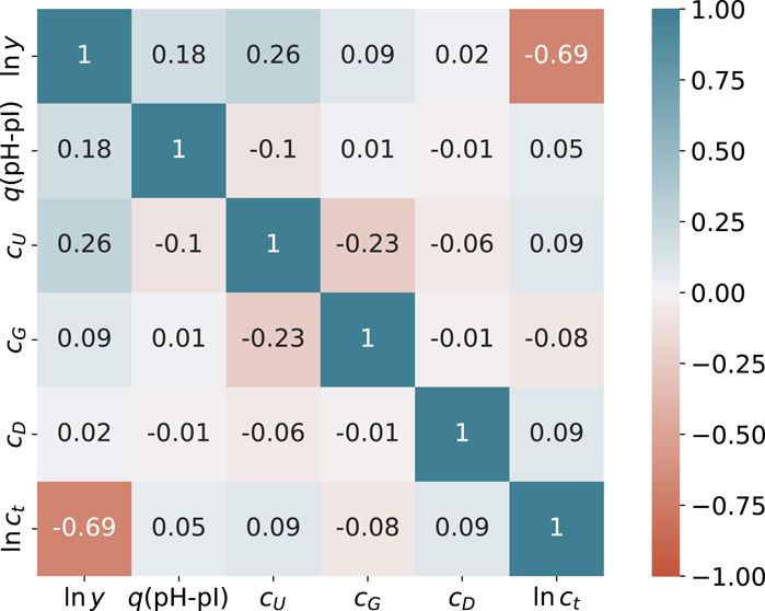
FIGURE 1. Pearson correlation coefficients r between feature values and ln y from the experimental data. The colors of the individual entries highlight the corresponding value of the Pearson correlation coefficient from r =1 (blue) via r =0 (white) to r =−1 (red).

As a next step, the corresponding supervised non-optimized machine learning and standard regression methods are assessed in order to predict the corresponding ln y values with regard to a k-fold cross-validation scheme including successive permutations of the training set (Gareth et al., 2013; Wong, 2015). As can be seen in the Supplementary Material, the highest predictive accuracy for a qualitative assessment of the non-optimized models is achieved for gradient boosting and decision tree-based methods. In more detail, histogram gradient boosting (HGB), extra trees (ET), gradient boosting (GB) and random forests (RF) show low nRMSE values between 0.19 and 0.21. The corresponding coefficients of determination between predicted and actual values vary between R² = 0.72–0.75. Noteworthy, ensemble boosting methods are ideally suited for non-linear regression problems like solubilization processes. Potential reasons for the high accuracy of decision tree-based models were recently published (Grinsztajn et al., 2022). In more detail, decision-tree based models do not overly smooth the solution in terms of predicted target values. Moreover, it was shown that uninformative features do not affect the performance metrics of decision-tree based models as much as for other machine learning approaches. In terms of such findings, it becomes clear that decision-tree based models often outperform kernel-based approaches in terms of predictive accuracies. It has to be noted that ensemble-based methods are also often robust against overfitting issues (Dietterich, 2000). Hence, time-consuming hyperoptimization tunings and validation checks are not of utmost importance.

In contrast to the good predictions of boosting models, standard linear regression methods like least-angle regression (LARS) or Lasso regression (LAS) show a rather poor performance (Supplementary Material). Interestingly, also standard artificial neural networks (ANNs) show a low predictive accuracy. It can be argued that further optimization of hyper parameters may improve the results. All other approaches show a reasonable or even good performance with nRMSE values between 0.26–0.22. As already discussed, the best performance can be observed for advanced decision tree-based ensemble models which reveals the underlying influence of non-linear contributions.

The corresponding predicted and experimental values for ln y from the HGB method are presented in Figure 2. We used a k-fold cross validation approach, where the training data consists of each N-1 data samples with one test data point from the total data set including N samples (Gareth et al., 2013; Wong, 2015). In more detail, each model M_j is trained with the feature data including the samples X = [x₁, x₂, …, x_j−1, x_j+1, …, x_N] and the associated target data Y = [y₁, y₂, …, y_j−1, y_j+1, …, y_N] and predicts the corresponding test target sample Y_j from X_j. As can be seen, X_j and Y_j are not part of the corresponding training data for model M_j. This procedure is repeated for all N models M₁, M₂, …, M_j and the corresponding predictions. Notably, a good agreement between the predicted and experimental values for all 0 > ln y > − 1.6 becomes obvious. All values are located within the experimental standard deviation σ(ln y) as denoted by the dashed blue lines. The corresponding good agreement can be rationalized by the large amount of training data in this range. Notable deviations in terms of one outlier with nRMSE $>1$ can only be observed for ln y ≤ −1.9 due to missing reference training data. Moreover, the good predictive accuracy is also highlighted by the reasonable value R² = 0.75 for the coefficient of determination. As shown in the supplementary material, similar conclusions can also be drawn for the prediction of a training data set of 38 samples using an 80/20 ratio split between training and test data. The RMSE values are of comparable quality. In consequence, it can be concluded that solubilization mechanisms and final yield values can be predicted with acceptable accuracy using machine learning approaches.

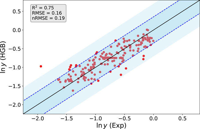
FIGURE 2. Predicted (HGB) and experimental values (Exp) for the logarithm of the yield ln y from the optimized HGB method. The straight line has a slope of one and the corresponding blue dotted lines reveal the experimental standard deviation σ(ln y). The lighter blue shaded regions demark a standard deviation of 2σ(ln y).

4.2 Feature importance analysis and explainable machine learning

Due to the reasonable predictive accuracy of certain machine learning models, it can be concluded that the evaluation of feature importances might provide some further insights into the underlying mechanisms of solubilization. In terms of such considerations, we evaluated all training data with the HGB and the ET method in accordance with the SHAP values. The results for the HGB model are shown in the Supplementary Material. As expected, the accuracies of the HGB and the ET model for training data with R² = 0.91 (HGB), R² = 0.99 (ET), nRMSE = 0.30 (HGB) and nRMSE = 0.10 (ET) are higher when compared to the predictions from the k-fold cross-validation approach which rationalizes the validity of the following feature analysis.

As a first step, the corresponding Gini feature importance values as calculated from the ET method are presented in Figure 3. As can be seen, the results confirm the dominant influence of the total protein concentration c_t in accordance with the correlation coefficients shown in Figure 1, followed by the urea concentration c_U and the fraction of protonated titrable groups q(pH-pI). With regard to rather low values, the DTT and guanidinium hydrochloride concentrations have negligible influences. It should be noted that the protein’s native structure is characterized by only a very small number of disulfide bonds. This property explains the vanishing influence as well as the relatively low concentration of DTT as a reducing agent in this context. Furthermore, it is well-known that guanidinium hydrochloride is a very potent destabilizing agent. However, in combination with urea it shows a rather complex aggregation behavior around the protein (Oprzeska-Zingrebe and Smiatek, 2021, 2022; Miranda-Quintana and Smiatek, 2021). Accordingly, higher concentrations of guanidinium hydrochloride could probably exert a stronger influence in terms of feature importance. However, it should be noted that this effect is represented here by the somewhat milder denaturation conditions in the presence of urea. In consequence, it can be concluded that the low feature importance of the guanidinium hydrochloride concentration can be rationalized by its corresponding low concentration. These results are also confirmed by the values from the ELI5 analysis which are shown in the Supplementary Material.

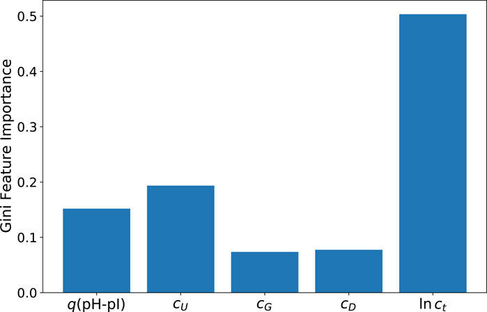
FIGURE 3. Gini feature importance values for predictions of the extra trees (ET) model for the protein yield ln y.

Similar conclusions can also be drawn in terms of example decision pathways for an extra trees model with a maximum tree depth of 4 as shown in the Supplementary Material. It becomes obvious that the first decision criterion defines a total protein concentration of ln c_t = 1.39. This value separates between high and low yield branches whereas further criteria based on individual values of q(pH-pI) and c_U are of minor importance and thus lead to different subclassifications.

The corresponding results for the SHAP value analysis with regard to the final yield values ln y from a HGB model are shown in Figure 4. The color-coded beeswarm plot with the associated contributions of SHAP values are depicted in the top panel. The beeswarm plot aims to provide an information-dense summary for the most important features in terms of model predictions for each data instance. Each data instance is represented by a single dot on each feature row. The horizontal position of the dot is determined by the SHAP value of the corresponding feature. In addition, the color illustrates the original value of a feature. Thus, the beeswarm plot highlights the importance or contribution of the features for the whole dataset. As already discussed, it becomes obvious that the largest influence is represented by the total protein concentration, followed by the urea concentration and the amount of protonated titrable groups. Moreover, it can be seen that the total protein concentration has a negative influence on the final yield value. Thus, low values of c_t lead to positive SHAP values and vice versa. Such findings are unique for the total protein concentration while all other factors show a positive correlation. In terms of a molecular understanding, it has to be noted that the solubilization process itself is a rather complex process due to contributions from interfacial phenomena, the composition of the solution as well as further intermolecular mechanisms. Moreover, the individual features and their contributions on the model predictions are ordered in terms of their importance from top to bottom. This ordering is calculated from the mean absolute SHAP value for each feature. In general, such an approach is strongly determined by the broad average impact of the feature while rare maximum or minimum values do not contribute significantly. The corresponding mean absolute SHAP values are presented in the bottom of Figure 4 for reasons of consistency. It clearly can be seen that the total protein concentration dominates the feature importance, followed by the urea concentration and q(pH-pI). The contributions from c_G and c_D are of minor importance in agreement with the p values from the previous correlation analysis.

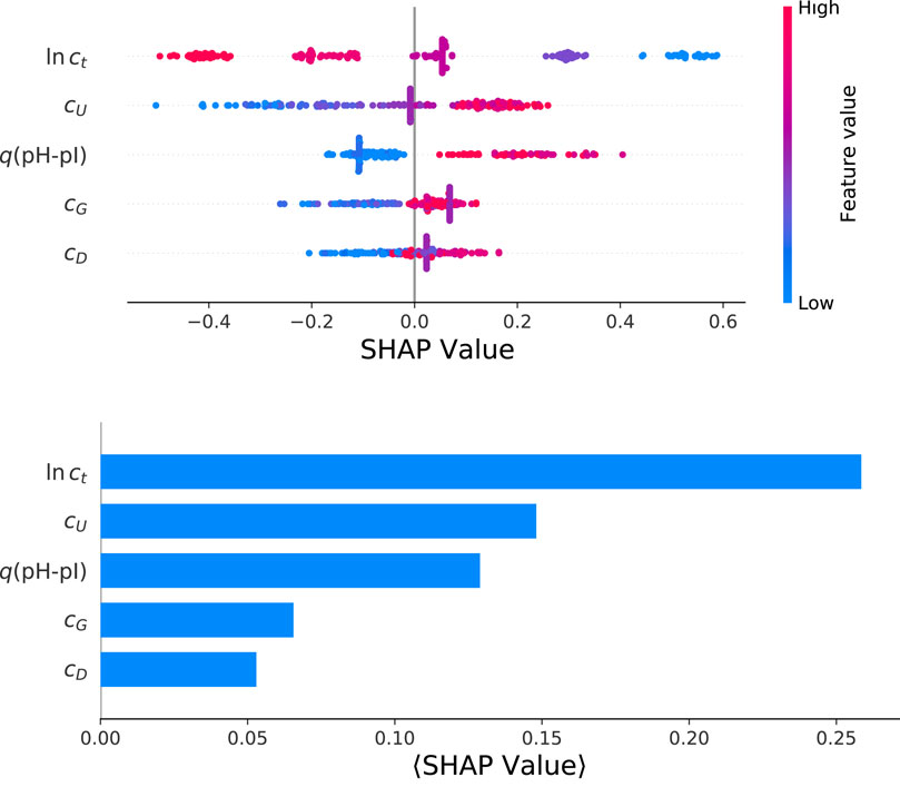
FIGURE 4. Color-coded heatmap for a beeswarm plot of individual SHAP values for the optimized HGB model (top panel) and mean absolute SHAP values as calculated for the target value ln y.

For a more detailed analysis, we present the corresponding SHAP value dependency plots for the total protein concentration in Figure 5. In general, SHAP dependency plots as shown in Figures 5, 6 highlight the effect of a single feature on the model predictions. Each dot corresponds to a single prediction from the dataset and the position on the horizontal axis denotes the corresponding actual value of the feature. In contrast, the vertical axis shows the SHAP value for that feature and its impact on the prediction. In general, a slope along the points in the dependency plots enables to identify positive, negative or no correlations with the corresponding target parameter. It clearly can be seen in Figure 5 that the aforementioned negative correlation (Figure 4) can be interpreted as an inverse relation between the total protein concentration and the final yield value ln y. Hence, for increasing total protein concentrations, one can observe a linear decrease of the SHAP values. The corresponding mechanism can be explained as follows. In general, the yield is defined by

which corresponds to the ratio between the number of free (solubilized) protein chains N_f and the total number of chains N_t. With regard to the fact that inclusion bodies show a rather poor solubility, one can assume that individual inclusion bodies aggregate in order to form larger moieties. Hence, the dissolution of free chains mainly occurs at the solvent accessible surface area of these compounds in agreement with previous assumptions (Walther et al., 2013).

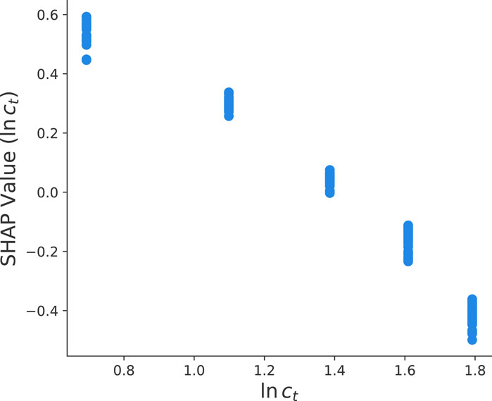
FIGURE 5. SHAP value dependency plot between the total protein concentration ln c_t and the final yield value ln y as calculated from the optimized HGB method.

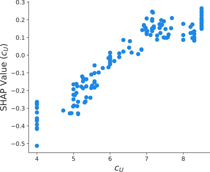
FIGURE 6. SHAP value dependency plot between the urea concentration c_U and the final yield value ln y from the optimized HGB method.

The number of free protein chains can be written as $N_f=c_p{R}_I^{2}d$ with the local concentration of proteins in the aggregated inclusion body c_p, the corresponding spherical radius R_I of the aggregate and the penetration or dissolution depth d. Moreover, it is assumed that the inner region of the compound remains unaffected by dissolution such that $N_t\approx c_p{R}_I^3$ with R_I ≫ d. In consequence, we can rewrite Eq. 6 according to

which reveals that aggregated inclusion bodies with larger radii result in lower yield values. Furthermore, it is assumed that d is constant after a fixed time interval. With regard to the fact that the radius scales as $R_I=N_t^{1/3}/c_p^{1/3}$, one obtains after insertion into Eq. 7 the following relation

which clearly shows that the final yield value depends inversely on the total protein concentration N_t ∼ c_t as represented by ln y ∼ − ln(c_t) in agreement with Figure 5. Here, we assume that d is constant after a fixed time interval and that aggregates show a highest packing fraction leading to fixed values of c_p.

Moreover, it is well known that the presence of urea induces a structural destabilization of proteins. Recent articles rationalized this phenomena with preferential binding and exclusion mechanisms (Smiatek, 2017; Oprzeska-Zingrebe and Smiatek, 2018; Miranda-Quintana and Smiatek, 2021). As can be seen in Figure 6, one observes increasing SHAP values and thus a positive trend of ln y for increasing urea concentrations. Moreover, it can be seen that for urea concentrations larger than 8 mol/L, a saturation behavior becomes evident. As an explanation, we refer to co-solute induced destabilization effects as discussed in Oprzeska-Zingrebe and Smiatek (2018); Smiatek (2017). In more detail, it is assumed that the ratio of destabilized and stable proteins K_cs can be written as

with the derivative of the thermodynamic activity a₃₃, the difference in the preferential binding coefficients Δν₂₃ and the ratio of destabilized and stable proteins K₀ in absence of any co-solutes (Smiatek, 2017; Oprzeska-Zingrebe and Smiatek, 2018; Smiatek et al., 2018). For certain proteins, it was discussed that the partial molar volumes and the solvent-accessible surface area upon unfolding do not change significantly according to Δν₂₃ = c_UΔG₂₃ (Smiatek et al., 2018; Krishnamoorthy et al., 2018a), such that the previous relation can be approximated by

with the difference in the Kirkwood-Buff integrals ΔG₂₃ (Oprzeska-Zingrebe and Smiatek, 2018). In addition to stable and destabilized proteins, one can apply the same relation for the fraction of dissolved and bound proteins (Smiatek et al., 2018). Under the assumption that N_f ≪ N_t, it thus follows that K_cs ≈ y and K₀ ≈ y₀. For high co-solute concentrations, it was further discussed that a₃₃ → 0 due to stability conditions (Krishnamoorthy et al., 2018b). Hence, the exponential factor in Eq. 10 can be linearized according to

which highlights the linear contribution y ∼ c_U between the urea concentration and the final yield value in good agreement with Figure 6.

In our previous discussion, it was also highlighted that the fraction of protonated titrable groups has a positive influence on the final yield values. In accordance with Eq. 2, it becomes clear that q(pH-pI) decreases with increasing pH values. Moreover, it is known that the isoelectric point with pI = 8.4 corresponds to a net-uncharged protein. The clear distinction between pH values below and above the pI value in terms of the SHAP dependency plot can be seen in Figure 7. In more detail, q(pH − pI) < 0.5 as represented by pH $<8.4$ results in negative SHAP values and thus lower yields and vice versa. The reason for this observation might be related to electrostatic repulsion between the charged groups of the protein (Smiatek et al., 2020). Thus, we assume that for high or low pH values, depending on the net amount of basic or acidic groups in the protein, the electrostatic repulsion fosters the dissolution of the protein in order to minimize non-favorable interactions. As also illustrated in Figure 7, significant contributions for a net-uncharged protein at pH = 8.4 leading to q(pH − pI) = 0.5 are absent.

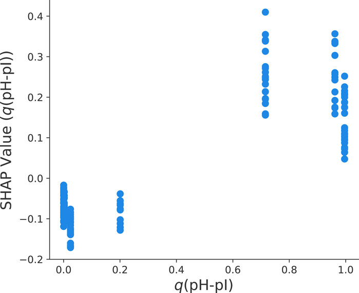
FIGURE 7. Dependency plot of SHAP values for the fraction of titrable groups q(pH − pI) and the final yield value ln y for the optimized HGB model.

The combination of the previous considerations in terms of Eqs 2, 8, 11 results in

which condenses all previous results in one analytic expression. In order to assess the validity of Eq. 12, we plotted all experimental data points onto a master curve as shown in Figure 8. In order to minimize fluctuating electrostatic repulsions, we chose nearly constant and high pH values with pH $\ge 10$ as well as high urea concentrations with c_U ≥ 7.55 mol/L. The corresponding 27 data points are then scaled in terms of a normal distribution and compared to Eq. 12. As can be seen in Figure 8, the theoretically predicted values nicely follow the proposed scaling relation. It has to be noted that the corresponding influences for different proteins and modalities upon solubilization may vary, such that the obtained results are not generally transferable without proper assessment. Nevertheless, we have proven strong evidence that explainable machine learning approaches provide deeper insights into the molecular mechanisms and correlations of solubilization processes.

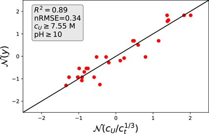
FIGURE 8. Theoretical estimates from Eq. 12 and actual values: The corresponding data points were selected for high urea concentrations and high pH values. All values are scaled in terms of normal distributions.

5 Discussion of results

In the previous sections, we developed a machine learning model to predict yield values based on some input features. We were able to show that an optimized Histogram Gradient Boosting (HGB) model enables the most accurate predictions. The underlying data for training and testing of the model were obtained from a Design of Experiments study. Overall, the model predictions show sufficient accuracy. The general trends are reproduced despite some minor inaccuracies for certain outliers. Previous statistical analysis of the experimental data already showed that the correlation coefficients between the feature and the target value do not reveal a particularly significant correlation. Accordingly, we could already assume in advance that the models would only allow meaningful predictions to a certain extent. To compensate for this drawback, we applied some methods of explainable machine learning. Although such approaches cannot increase the accuracy, the results provide fundamental insights into the feature importance for the model predictions. We observed that in particular the total protein concentration as well as the urea concentration and the degree of charge of the protein due to the adjusted pH value are of decisive importance for the yield value predictions. The influence of other co-solutes is negligible due to their low concentration. As part of the explainable machine learning approach, we were therefore able to examine data-driven models on a scientific basis. Accordingly, we were able to set up scientific hypotheses for the underlying mechanisms (Smiatek et al., 2021b), which provided a rationale for the observed feature importance values. These scientific hypotheses were then merged into Eq. 12, which allows for a formal mathematical description of the influence of various parameters on yield values.

In general, it cannot be assumed that a single machine learning model is suitable to predict different yields for different proteins in different solubilization procedures. The differences in the charges and the interaction with co-solutes are sometimes so significantly different that the trends can sometimes even reverse. Accordingly, the general transferability of machine learning models is usually not given, so that the gain in knowledge is often very small. Accordingly, experimental data must be recorded again for new proteins and their inclusion bodies, so that the reduction in laboratory activities is usually not given. However, basic principles can be recognized by means of the analytical equation and the corresponding scientific hypotheses. These principles may differ slightly for individual proteins, but can now be estimated in advance using the analytical description. Hence, important influencing factors can be postulated, especially when planning the experiments. We were also able to show that the purely data-driven models can be subjected to scientific hypothesis formation, which makes the results more robust and more straightforward to understand.

6 Summary and conclusion

We studied the potential influences of certain process parameters on the solubilization of inclusion bodies in terms of explainable machine learning approaches. The corresponding final yield values after solubilization are crucially affected by the total protein concentration, the urea concentration and the amount of protonated titrable groups as affected by the actual pH value. The models with highest predictive accuracies are boosting ensemble-based approaches with nRMSE values around 0.19. The corresponding SHAP values show that the total protein concentration, the actual urea concentration as well as the fraction of protonated titrable groups dominate the final yield value. All other contributions like the DTT and guanidinium hydrochloride concentration are of minor importance. A more detailed analysis of SHAP dependecies also highlights an inverse relation between the total protein concentration and the yield values in contrast to the urea concentration and the amount of protonated titrable groups.

Based on these explainable machine learning observations, we proposed an analytic expression to rationalize these findings. The inverse relation for the total protein concentration can be understood with regard to surface solvation effects which inversely scale with the total protein concentration. The growing SHAP values for the urea concentration can be understood by the preferential binding and exclusion mechanisms for co-solutes. The direct interaction of urea molecules with the inclusion body thus favors dissolution mechanisms and hence larger yield values. Finally, larger fractions of protonated titrable groups result in stronger electrostatic repulsion effects between the proteins which facilitate the dissolution of the inclusion body. The corresponding assumptions can be summarized in terms of an analytic expression which shows a reasonable agreement with the experimental data. Although it has to be noted that the corresponding dependencies crucially rely on the nature of the protein and the inclusion bodies, our approach demonstrates a meaningful pathway towards a deeper understanding and optimization of solubilization conditions. It can be assumed that the underlying mechanisms vary through the individual contributions of the influencing factors for different proteins. Typical examples would be the influence of the pH value on different pI values of proteins as well as the importance of reducing reagents such as DTT at different amounts of disulfide bonds. Nevertheless, it can be expected that the presented machine learning models in combination with feature analysis can make these slightly varying relationships interpretable with similar accuracy as in this study. Accordingly, our work highlights an exemplary and generic approach to understand in detail the phenomena of solubilization for the individual proteins and solutions. The use of explainable machine learning approaches thus allows us to develop models with high predictive accuracy but also to gain deeper insights into the underlying correlations of the mechanisms. Hence, it has to be mentioned that the use of explainable machine learning does not increase the prediction accuracy of the model. However, there is the possibility that the results of non-parametric models can be assessed and evaluated in their justification with regard to individual feature correlations. This procedure corresponds to the scientific method, so that the results of purely data-driven models can be translated into scientific hypotheses and made correspondingly falsifiable (Smiatek et al., 2021b). In this context, the use of explainable machine learning has allowed us to derive an analytical equation (Eq. 12). As we have shown, this analytical equation can also be derived separately from fundamental principles, with the SHAP analysis being able to contribute profitably to the identification of these mechanisms. The advantage of such an equation lies in its falsifiability and its potential for transfer to other projects. From this it can be assumed that new projects can be started with prior knowledge, so that material can be saved and the work can be reduced. In consequence, explainable machine learning provides a deeper process understanding and knowledge which is beneficial for different unit operations in biopharmaceutical manufacturing.

Data availability statement

The data analyzed in this study is subject to the following licenses/restrictions: jens.smiatek@boehringer-ingelheim.com. Requests to access these datasets should be directed to cornelia.walther@boehringer-ingelheim.com.

Author contributions

JS, CW, and MM conducted the study and analyzed the results. All authors contributed to the article and approved the submitted version.

Funding

This research was funded by Boehringer Ingelheim Pharma GmbH & Co. KG and Boehringer Ingelheim RCV GmbH & Co KG.

Acknowledgments

The authors thank Christina Yassouridis, Hermann Schuchnigg, I-Ting Ho, Milena Matysik, Liliana Montano Herrera, Ralph Guderlei, Michael Laussegger, and Bernhard Schrantz for valuable discussions.

Conflict of interest

Authors CW, MM, AF, A-LT, MV, and CB were employed by Boehringer Ingelheim RCV GmbH & Co. KG. Author A-LT was employed by Baxalta Innovations GmbH, Takeda Group. Authors AJ, EB, and JS were employed by Boehringer Ingelheim Pharma GmbH & Co. KG.

The remaining authors declare that the research was conducted in the absence of any commercial or financial relationships that could be construed as a potential conflict of interest.

Publisher’s note

All claims expressed in this article are solely those of the authors and do not necessarily represent those of their affiliated organizations, or those of the publisher, the editors and the reviewers. Any product that may be evaluated in this article, or claim that may be made by its manufacturer, is not guaranteed or endorsed by the publisher.

Supplementary material

The Supplementary Material for this article can be found online at: https://www.frontiersin.org/articles/10.3389/fceng.2023.1227620/full#supplementary-material

References

Agarwal, N., and Das, S. “Interpretable machine learning tools: A survey,” in Proceedings of the 2020 IEEE Symposium Series on Computational Intelligence (SSCI), Canberra, ACT, Australia, December 2020, 1528–1534.
Belle, V., and Papantonis, I. (2021). Principles and practice of explainable machine learning. Front. Big Data 4, 688969. doi:10.3389/fdata.2021.688969
Blaser, R., and Fryzlewicz, P. (2016). Random rotation ensembles. J. Mach. Learn. Res. 17, 126–151. doi:10.5555/2946645.2946649
Bowden, G. A., Paredes, A. M., and Georgiou, G. (1991). Structure and morphology of protein inclusion bodies in escherichia coli. Biotechnol 9, 725–730. doi:10.1038/nbt0891-725
Breiman, L., Friedman, J., Stone, C. J., and Olshen, R. A. (1984). Classification and regression trees. Boca Raton, Florida, United States: CRC Press.
Brownlee, J. (2016). XGBoost with python: Gradient boosted trees with XGBoost and scikit-learn. Vermont, Victoria, Australia: Machine Learning Mastery.,
Burkart, N., and Huber, M. F. (2021). A survey on the explainability of supervised machine learning. J. Art. Intell. Res. 70, 245–317. doi:10.1613/jair.1.12228
Clark, E. D. B. (1998). Refolding of recombinant proteins. Curr. Opin. Biotechnol. 9, 157–163. doi:10.1016/s0958-1669(98)80109-2
Dietterich, T. G. (2000). “Ensemble methods in machine learning,” in International workshop on multiple classifier systems (Berlin, Germany: Springer), 1–15.
Feng, D.-C., Wang, W.-J., Mangalathu, S., Hu, G., and Wu, T. (2021). Implementing ensemble learning methods to predict the shear strength of rc deep beams with/without web reinforcements. Eng. Struct. 235, 111979. doi:10.1016/j.engstruct.2021.111979
Freydell, E. J., Ottens, M., Eppink, M., van Dedem, G., and van der Wielen, L. (2007). Efficient solubilization of inclusion bodies. Biotechnol. J. 2, 678–684. doi:10.1002/biot.200700046
Gareth, J., Daniela, W., Trevor, H., and Robert, T. (2013). An introduction to statistical learning: With applications in R. Berlin, Germany: Spinger.
Grinsztajn, L., Oyallon, E., and Varoquaux, G. (2022). Why do tree-based models still outperform deep learning on tabular data? https://arxiv.org/abs/2207.08815.
Gunning, D., Stefik, M., Choi, J., Miller, T., Stumpf, S., and Yang, G.-Z. (2019). Xai—Explainable artificial intelligence. Sci. Robot. 4, 7120. doi:10.1126/scirobotics.aay7120
Harris, C. R., Millman, K. J., van der Walt, S. J., Gommers, R., Virtanen, P., Cournapeau, D., et al. (2020). Array programming with NumPy. Nature 585, 357–362. doi:10.1038/s41586-020-2649-2
Holzinger, A., Kieseberg, P., Weippl, E., and Tjoa, A. M. (2018). “Current advances, trends and challenges of machine learning and knowledge extraction: From machine learning to explainable ai,” in International cross-domain conference for machine learning and knowledge extraction (Berlin, Germany: Springer), 1–8.
Kailkhura, B., Gallagher, B., Kim, S., Hiszpanski, A., and Han, T. (2019). Reliable and explainable machine-learning methods for accelerated material discovery. NPJ Comput. Mat. 5, 108–109. doi:10.1038/s41524-019-0248-2
Krishnamoorthy, A. N., Holm, C., and Smiatek, J. (2018a). Influence of cosolutes on chemical equilibrium: A kirkwood–buff theory for ion pair association–dissociation processes in ternary electrolyte solutions. J. Phys. Chem. C 122, 10293–10302. doi:10.1021/acs.jpcc.7b12255
Krishnamoorthy, A. N., Oldiges, K., Winter, M., Heuer, A., Cekic-Laskovic, I., Holm, C., et al. (2018b). Electrolyte solvents for high voltage lithium ion batteries: Ion correlation and specific anion effects in adiponitrile. Phys. Chem. Chem. Phys. 20, 25701–25715. doi:10.1039/c8cp04102d
Landsgesell, J., Holm, C., and Smiatek, J. (2017). Wang–landau reaction ensemble method: Simulation of weak polyelectrolytes and general acid–base reactions. J. Chem. Theo. Comput. 13, 852–862. doi:10.1021/acs.jctc.6b00791
Linardatos, P., Papastefanopoulos, V., and Kotsiantis, S. (2020). Explainable ai: A review of machine learning interpretability methods. Entropy 23, 18. doi:10.3390/e23010018
Lundberg, S. M., and Lee, S.-I. (2017). A unified approach to interpreting model predictions. Adv. Neural. Inf. Proc. Sys. 30. doi:10.48550/arXiv.1705.07874
Miranda-Quintana, R. A., and Smiatek, J. (2021). Electronic properties of protein destabilizers and stabilizers: Implications for preferential binding and exclusion mechanisms. J. Phys. Chem. B 125, 11857–11868. doi:10.1021/acs.jpcb.1c06295
Molnar, C., Casalicchio, G., and Bischl, B. “Interpretable machine learning–a brief history, state-of-the-art and challenges,” in Proceedings of the Joint European Conference on Machine Learning and Knowledge Discovery in Databases, Ghent, Belgium, September 2020, 417–431.
Montano Herrera, L., Eilert, T., Ho, I.-T., Matysik, M., Laussegger, M., Guderlei, R., et al. (2022). Holistic process models: A bayesian predictive ensemble method for single and coupled unit operation models. Processes 10, 662. doi:10.3390/pr10040662
Oprzeska-Zingrebe, E. A., and Smiatek, J. (2022). Basket-type g-quadruplex with two tetrads in the presence of tmao and urea: A molecular dynamics study. J. Mol. Struct. 1274, 134375. doi:10.1016/j.molstruc.2022.134375
Oprzeska-Zingrebe, E. A., and Smiatek, J. (2018). Aqueous ionic liquids in comparison with standard co-solutes. Biophys. Rev. 10, 809–824. doi:10.1007/s12551-018-0414-7
Oprzeska-Zingrebe, E. A., and Smiatek, J. (2021). Interactions of a dna g-quadruplex with tmao and urea: A molecular dynamics study on co-solute compensation mechanisms. Phys. Chem. Chem. Phys. 23, 1254–1264. doi:10.1039/d0cp05356b
Oviedo, F., Ferres, J. L., Buonassisi, T., and Butler, K. T. (2022). Interpretable and explainable machine learning for materials science and chemistry. Acc. Mat. Res. 3, 597–607. doi:10.1021/accountsmr.1c00244
Pedregosa, F., Varoquaux, G., Gramfort, A., Michel, V., Thirion, B., Grisel, O., et al. (2011). Scikit-learn: Machine learning in Python. J. Mach. Learn. Res. 12, 2825–2830. doi:10.5555/1953048.2078195
Pilania, G. (2021). Machine learning in materials science: From explainable predictions to autonomous design. Comput. Mat. Sci. 193, 110360. doi:10.1016/j.commatsci.2021.110360
Politis, S. N., Colombo, P., Colombo, G., and Rekkas, M. D. (2017). Design of experiments (doe) in pharmaceutical development. Drug Dev. indust. Pharm. 43, 889–901. doi:10.1080/03639045.2017.1291672
Ramón, A., Señorale, M., and Marín, M. (2014). Inclusion bodies: Not that bad. Front. Microbiol. 5, 56. doi:10.3389/fmicb.2014.00056
Ribeiro, M. T., Singh, S., and Guestrin, C. (2016). Model-agnostic interpretability of machine learning. https://arxiv.org/abs/1606.05386.
Roscher, R., Bohn, B., Duarte, M. F., and Garcke, J. (2020). Explainable machine learning for scientific insights and discoveries. Ieee Access 8, 42200–42216. doi:10.1109/access.2020.2976199
Shapley, L. (1953). “Quota solutions op n-person games,” in Contributions to the theory of games (Santa Monica, CL, USA: The Rand Corporation).
Singh, S. M., and Panda, A. K. (2005). Solubilization and refolding of bacterial inclusion body proteins. J. Biosci. Bioeng. 99, 303–310. doi:10.1263/jbb.99.303
Singhvi, P., Saneja, A., Srichandan, S., and Panda, A. K. (2020). Bacterial inclusion bodies: A treasure trove of bioactive proteins. Trends Biotechnol. 38, 474–486. doi:10.1016/j.tibtech.2019.12.011
Smiatek, J. (2017). Aqueous ionic liquids and their effects on protein structures: An overview on recent theoretical and experimental results. J. Phys. Condens. Matter 29, 233001. doi:10.1088/1361-648x/aa6c9d
Smiatek, J., Clemens, C., Herrera, L. M., Arnold, S., Knapp, B., Presser, B., et al. (2021a). Generic and specific recurrent neural network models: Applications for large and small scale biopharmaceutical upstream processes. Biotechnol. Rep. 31, e00640. doi:10.1016/j.btre.2021.e00640
Smiatek, J., Heuer, A., and Winter, M. (2018). Properties of ion complexes and their impact on charge transport in organic solvent-based electrolyte solutions for lithium batteries: Insights from a theoretical perspective. Batteries 4, 62. doi:10.3390/batteries4040062
Smiatek, J., Jung, A., and Bluhmki, E. (2020). Towards a digital bioprocess replica: Computational approaches in biopharmaceutical development and manufacturing. Trends Biotechnol. 38, 1141–1153. doi:10.1016/j.tibtech.2020.05.008
Smiatek, J., Jung, A., and Bluhmki, E. (2021b). Validation is not verification: Precise terminology and scientific methods in bioprocess modeling. Trends Biotechnol. 39, 1117–1119. doi:10.1016/j.tibtech.2021.04.003
Štrumbelj, E., and Kononenko, I. (2014). Explaining prediction models and individual predictions with feature contributions. Knowl. Info. Sys. 41, 647–665. doi:10.1007/s10115-013-0679-x
Sudret, B. (2008). Global sensitivity analysis using polynomial chaos expansions. Reliab. Eng. Sys. Saf. 93, 964–979. doi:10.1016/j.ress.2007.04.002
Valax, P., and Georgiou, G. (1993). Molecular characterization of β-lactamase inclusion bodies produced in escherichia coli. 1. composition. Biotechnol. Prog. 9, 539–547. doi:10.1021/bp00023a014
Van Rossum, G., and Drake, F. L. (2009). Python 3 reference manual. Scotts Valley, CA, USA: CreateSpace.
Wakjira, T. G., Al-Hamrani, A., Ebead, U., and Alnahhal, W. (2022). Shear capacity prediction of frp-rc beams using single and ensenble explainable machine learning models. Comp. Struct. 287, 115381. doi:10.1016/j.compstruct.2022.115381
Walther, C., Mayer, S., Sekot, G., Antos, D., Hahn, R., Jungbauer, A., et al. (2013). Mechanism and model for solubilization of inclusion bodies. Chem. Eng. Sci. 101, 631–641. doi:10.1016/j.ces.2013.07.026
Walther, C., Mayer, S., Trefilov, A., Sekot, G., Hahn, R., Jungbauer, A., et al. (2014). Prediction of inclusion body solubilization from shaken to stirred reactors. Biotechnol. Bioeng. 111, 84–94. doi:10.1002/bit.24998
Walther, C., Voigtmann, M., Bruna, E., Abusnina, A., Tscheließnig, A.-L., Allmer, M., et al. (2022). Smart process development: Application of machine-learning and integrated process modeling for inclusion body purification processes. Biotechnol. Prog. 38, e3249. doi:10.1002/btpr.3249
Wes McKinney, “Data structures for statistical computing in Python,” in Proceedings of the 9th Python in Science Conference, Austin, Texas, June 2010. doi:10.25080/Majora-92bf1922-00a
Wong, T.-T. (2015). Performance evaluation of classification algorithms by k-fold and leave-one-out cross validation. Pattern Recogn. 48, 2839–2846. doi:10.1016/j.patcog.2015.03.009
Keywords: inclusion bodies, refolding, solubilization, SHAP (shapley additive explanation), explainable machine learning
Citation: Walther C, Martinetz MC, Friedrich A, Tscheließnig A-L, Voigtmann M, Jung A, Brocard C, Bluhmki E and Smiatek J (2023) Solubilization of inclusion bodies: insights from explainable machine learning approaches. Front. Chem. Eng. 5:1227620. doi: 10.3389/fceng.2023.1227620
Received: 23 May 2023; Accepted: 20 July 2023;
Published: 07 August 2023.
Edited by:
Jin Wang, Auburn University, United StatesReviewed by:
Joel Paulson, The Ohio State University, United StatesGefei Chen, Karolinska Institutet (KI), Sweden
Copyright © 2023 Walther, Martinetz, Friedrich, Tscheließnig, Voigtmann, Jung, Brocard, Bluhmki and Smiatek. This is an open-access article distributed under the terms of the Creative Commons Attribution License (CC BY). The use, distribution or reproduction in other forums is permitted, provided the original author(s) and the copyright owner(s) are credited and that the original publication in this journal is cited, in accordance with accepted academic practice. No use, distribution or reproduction is permitted which does not comply with these terms.
*Correspondence: Cornelia Walther, cornelia.walther@boehringer-ingelheim.com; Jens Smiatek, jens.smiatek@boehringer-ingelheim.com