Beyond the Ubiquitous Relapse Curve: A Data-Informed Approach

Relapse to alcohol and other substances has generally been described by curves that resemble one another. However, these curves have been generated from the time to first use after a period of abstinence without regard to the movement of individuals into and out of drug use. Instead of measuring continuous abstinence, we considered post-treatment functioning as a more complicated phenomenon, describing how people move in and out of drinking states on a monthly basis over the course of a year. When we looked at time to first drink we observed the ubiquitous relapse curve. When we classified clients (N = 550) according to drinking state however, they frequently moved from one state to another with both abstinent and very heavy drinking states as being rather stable, and light or moderate drinking and heavy drinking being unstable. We found that clients with a family history of alcoholism were less likely to experience these unstable states. When we examined the distribution of cases crossed by the number of times clients switched states we found that a power function explained 83% of that relationship. Some of the remainder of the variance seems to be explained by the stable states of very heavy drinking and abstinence acting as attractors.

Introduction

Kirshenbaum et al. (2009) are to be applauded for their meta-analysis of the relapse curve. They found that the relapse curve for tobacco and alcohol, across a variety of studies, can be explained by the same mathematical expression. However, implicit in the examination of the relapse curve is the perspective that what follows the first drink or first smoke after treatment does not matter. The data of a person who drinks one drink 30 days after treatment and then is abstinent for the next 11 months, is treated the same as the data of a person who consumes a case of beer 30 days after treatment, and continues to drink a case of beer every day for the rest of the year. Marlatt (1985) appreciated the difference between a lapse and a relapse, and highlighted this distinction. In other instances, data-reduction is fostered by the necessity to optimize statistical power while employing a Bonferroni correction for the number of dependent measures. For instance, in Project MATCH Research Group (1997) there were only two primary dependent measures, drinks per drinking day and percent days abstinent. In Project COMBINE, the two primary outcome measures were percent days abstinent and time to heavy drinking (Anton et al., 2006). These summary variables obfuscate the specific clinical outcomes of individual clients, by using summary variables that may unnecessarily obscure drinking patterns.

In the present article, we utilized an inductive approach, conducting basic analyses with minimal assumptions, in order to determine patterns in drinking outcomes following treatment. This simple yet elegant approach may reveal patterns in the data that have only been hinted at by theorists in the past. A few of the assumptions that were utilized include that drinking across the whole year is clinically relevant, and that drinking behavior chunked into months (or a similar rubric) would be useful to examine. Based on the work of Del Boca et al. (2004) it was considered crucial to examine a whole number of weeks rather than 30 day increments, since alcohol consumption is anchored to the specific days of the week, and that a 30-day interval would introduce unnecessary error variance in the examination of consecutive “monthly” intervals. Further, while alcohol-related negative consequences are clinically relevant, we decided that the examination of alcohol-related negative consequences would over-complicate and possibly obfuscate the examination of patterns of drinking behavior. For the building blocks of our analyses we used the number of standard drink units consumed as determined through the Form-90 interview (Miller, 1996). The operationalization of heavy drinking as four or more drinks for women, and five or more drinks for men consumed on a single day has been widely accepted and routinely employed in a large number of studies (National Institute of Alcohol Abuse and Alcoholism, 2004; Anton et al., 2006; Barnett et al., 2007). Further, the operationalization of very heavy drinking days (a doubling of the prior cut-offs) is gaining increased acceptance (Karhuvaara et al., 2007; Arias et al., 2008).

Materials and Methods

Participants

This article consists of a re-analysis of the drinking data from the relapse replication and extension project (RREP; Lowman et al., 1996). This multi-site study was conducted to assess the reliability and validity of the Marlatt relapse classification system, and to test various aspects of the theoretical models proposed by Marlatt in his seminal work (e.g., Marlatt and Gordon, 1985). The entire sample of 563 was recruited from alcohol treatment programs in Albuquerque, NM; Buffalo, NY; Providence, RI, and surrounding areas. The research protocol was approved by the Institutional Review Boards of Brown University, the Research Institute on Addictions, and the University of New Mexico. Eligibility criteria included meeting current diagnostic criteria for DSM-III-R alcohol dependence or abuse as determined by the diagnostic interview schedule (Robins et al., 1988) and being 18 years of age or older. Ninety nine percent of the sample met criteria for current alcohol dependence. Intravenous drug use in the last 6 months was an exclusion criteria.

The average age of participants at baseline was 34.3 (SD = 8.7) years. Women were well represented (41%) and the sample consisted primarily of White (67%), African American (16%), and Latino (9%) clients. Three quarters of the sample was single or separated/divorced (41 and 34%, respectively). Sixty two percent of the sample was unemployed. Sixty percent of the sample had at least one prior detoxification treatment. The average age of first drink was 14.0 (SD = 3.8). Seventy one percent of the sample had used at least one illicit drug in the last 90 days, primarily cocaine (44%), marijuana (42%), and tranquilizers (29%). Tobacco use was common (86%). Forty three percent reported that at least one parent was an “alcoholic.”

Materials

The primary measure used for these analyses is the Form-90, and in particular the Form-90 administered at the 2-, 4-, 6-, 8-, 10-, and 12-month follow-ups. The Form-90 (Miller, 1996) was administered every 60 days to yield a continuous calendar of drinking data. The reliability and validity of the Form-90 have been demonstrated (Tonigan et al., 1997). A subset of the items from the comprehensive drinker profile (Miller and Marlatt, 1984) were also administered, and the questions regarding the drinking behavior of one’s mother and father were used to determine family history (FH). Having an “alcoholic” parent qualified the client as FH+, while having a parent that is or was a problem drinker would not. Sample characteristics, design, and procedures for this naturalistic treatment outcome study are further described in Lowman et al. (1996). SPSS (Norusis, 2005) was used for the statistical analyses unless otherwise indicated.

Results

Five hundred and fifty participants (or 98% of the 563 enrolled) provided drinking outcome data for the first 28-day “month.” Follow-up rates based on the original 563 participants across the 13 “months” were 98, 98, 97, 97, 95, 94, 93, 92, 92, 91, 90, 88, and 88% respectively. The drinking behavior of each participant was classified as abstinent, light or moderate drinking (LMD), heavy drinking (HD), or very heavy drinking (VHD) for each of the successive 28-day intervals. The distribution for the first month consisted of 72.2% of the sample in an abstinent state, 4.0% in a LMD state, 5.8% in a heavy drinking state, and 18.0% in a very heavy drinking state. Distributions for these four drinking states for each of the 13 months are depicted in Figure 1. Starting with month 2, the distributions are fairly similar from month to month. This apparent consistency conceals the actual transition of participants between one state and another. While a participant in an abstinent state in a given month was likely to remain in that state in the following month 79–89% of the time depending on the particular month, and a participant that was in a VHD state in a given month was 70–78% likely to remain in that state in the successive month, the LMD and HD states were considerably less stable. Indeed, participants in these states were more likely to switch into a different state of drinking than to remain in the same state. For the successive pairs of months from Month 1 to Month 13, participants in a LMD state remained in that state 36% of the time. For the successive pairs of months, participants in a heavy drinking state remained in that state 43% of the time. The next most likely state for those in a LMD state to enter was abstinence (31%). The next most likely state for those in a heavy drinking state to enter was a VHD state (32%). (For the others transitioning out of a LMD state, 17% entered a heavy drinking state, and 16% entered a VHD state. For the others transitioning out of a HD state, 16% entered an abstinent state, and 9% entered a LMD state.) Across all 13 months, abstinence was the most common state (59%) followed by VHD (29%). The HD state (7%) and the LMD state (5%) were less common.

FIGURE 1

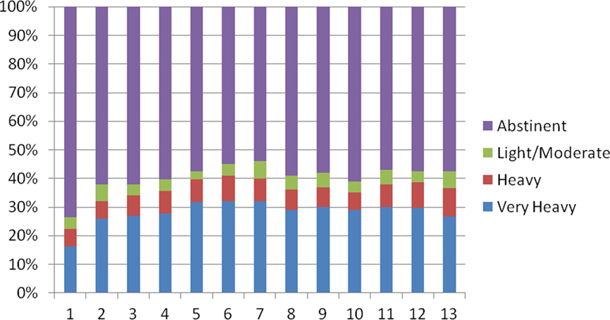
Figure 1. Drinking states as a percentage of the sample (y-axis) by follow-up month (x-axis).

The number of any transitions between states ranged from none (for the 26% that remained abstinent throughout the 13 months) to 11 (mean = 2.9, median = 2.0, SD = 2.6) and the distribution of this variable is depicted in Figure 2. The number of transitions appears to have a trimodal distribution, with modes at 0, 2, and 4. An examination of those ninety participants that had two and only two transitions revealed that 57% entered a VHD state and then returned to abstinence. Twenty percent entered a LMD state and then returned to abstinence. The remaining 23% rounded out most of the remaining possibilities: 2% entered a LMD state and then went to a HD state. None entered a LMD state and then entered VHD state. Four percent entered a HD state followed by abstinence. Two percent entered a HD state followed by a LMD state. Six percent entered a HD state followed by a VHD state. One percent entered a VHD state followed by a LMD state. Finally 8% entered a VHD state followed by a HD state. (It should be noted that the number of consecutive months in the second state, following abstinence, varied across participants.)

FIGURE 2

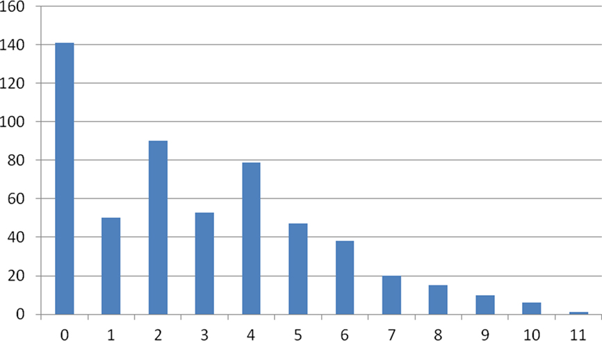
Figure 2. Number of transitions (x-axis) by number of cases (y-axis).

The following results are described to provide a specific example of how the more general results may be applied. It was hypothesized, that FH+ participants would be less likely to experience the unstable states of LMD and HD, than FH− participants. As hypothesized, FH+ clients were less likely to experience LMD states (4% of the time) than FH− clients [5% of the time, χ²(1, N = 6623) = 5.33, p < 0.05, where N is the number of client months] and less likely to experience HD states [6% versus 8%, χ²(1, N = 6623) = 11.97, p < 0.001]. In addition, FH+ clients were more likely to experience abstinence states [62% versus 58%, χ²(1, N = 6623) = 12.97, p < 0.001]. There was no difference in the likelihood of experiencing VHD states [28% for FH+ and 29% for FH−, χ²(1, N = 6623) = 0.72, p = 0.40].

Next, an examination of the distribution of the number of cases crossed by the number of transitions (Figure 2) suggested a power function, and this was confirmed, in that the log₁₀ of the number of cases was inversely correlated [r(10) = −0.91] with the number of switches (Figure 3) indicating that a power function explains 83% of the relationship between these two variables. We also tested whether other models might fit the data better using EasyFit 5.5 software available at www.mathwave.com. The Log Pearson 3 distribution (identical to the power relationship we found) was compared to the Triangular distribution (which appears to fit the data well by visual inspection) and to the Weibull distribution. According to the Anderson–Darling fit statistic, the Log Pearson 3 distribution fit the data best (fit statistics of 3.7, 4.2, and 4.6, for the Log Pearson 3, Triangular, and Weibull distributions, respectively, with a lower fit statistic indicating a better fit).

FIGURE 3

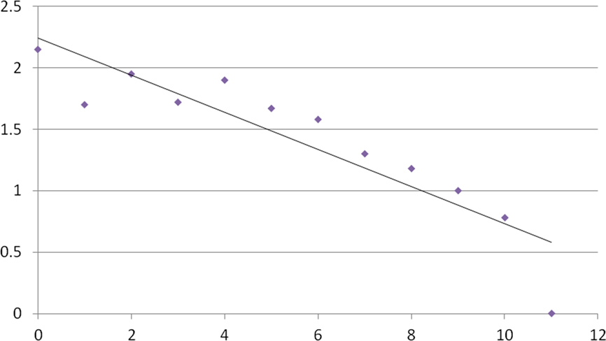
Figure 3. Number of transitions (x-axis) by log₁₀ of cases (y-axis) data and trendline.

Finally, since the last known state of a client may be the most clinically relevant, we examined the endpoint for each of the 550 participants with follow-up data. Fifty seven percent were abstinent, 6% were light or moderate drinkers, 10% were heavy drinkers, and 28% were very heavy drinkers. This endpoint state was plotted by the number of transitions in Figure 4. In this figure all of the participants that did not undergo a state transition were still abstinent for the last month. Conversely, the one client that underwent eleven state transitions, was in a very heavy drinking state for the last month.

FIGURE 4

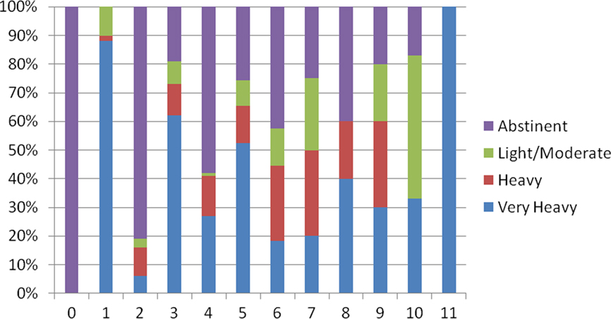
Figure 4. Endpoint by number of transitions (x-axis).

Discussion

In using an inductive approach to examine drinking following treatment, we uncovered a power function. More than 20 years ago, shortly after the popularity of Gleick’s (1987) bestseller Chaos, Skinner (1989) pointed toward the potential of chaos theory and associated hypotheses to inform the study of and treatment of addictive behavior. Barton (1994) described how chaos, non-linear dynamics, and self-organization could inform the study of a wide variety of psychological phenomena, and in particular, topics pertinent to clinical psychology. Manifestations of a number of complex systems across a wide variety of phenomena exhibit the “power function.” These diverse variables include the distribution of earthquakes ranked by the magnitude of the earthquakes, variation in cotton prices, the distribution of species extinctions ranked by the percentage of species extinguished (Bak, 1996), the distribution of cities based on population, and the distribution of simulated avalanches based on the size of the avalanche (Gribbin, 2004). For example, regarding the frequency of earthquakes and magnitude, for every 100 earthquakes of magnitude 5, there are approximately 10 earthquakes of magnitude 6, and approximately a single earthquake of magnitude 7 (Bak, 1996). One of the hallmarks of complex systems, phenomena determined by multiple inputs with subsequent iterations determined by proximal variables is this exact power function. A second hallmark of a complex system, is a sensitivity to initial conditions, which has been popularized as the butterfly effect. This observation suggests that small inputs may have large effects. A hallmark of dissipative systems in particular, is the ability to absorb energy with little change. These two seemingly contradictory characteristics will be discussed subsequently.

While the power function explains 83% of the variance in Figure 3, the remainder may be explained by the very heavy drinking state and abstinence acting as attractors. An attractor may be conceptualized as a resting area in a dynamic system. Examples of attractors include constructive interpersonal relations and destructive interpersonal relations (Vallacher et al., 2010). Horowitz (1986) hypothesized that clients with PTSD oscillate between the attractors of re-experiencing symptoms and avoidance/numbing symptoms. Similarly, manic episodes and depressed episodes may be viewed as two attractors. In this paper the abstinence state and the very heavy drinking state are the most common states as revealed by Figure 2. In addition, an examination of those clients exhibiting two switches revealed that 87% settled in the abstinent or very heavy drinking state. Further, as the sample moves from 0 transitions to four transitions, in Figure 4, the clients appear to oscillate between these two attractors. For a more thorough discussion of attractors, please see Barton (1994).

As opposed to the primarily descriptive analyses utilized in this article, trajectory analysis may impose a structure on the data such that a stable high group, a stable low group, a group that increases, and a group that decreases are frequently “detected” (Windle, 2008). The analyses employed here indicate that these profiles oversimplify the actual phenomena, with many clients exhibiting five or more transitions in a 13-month period. In this article we have demonstrated that the power function explains in excess of 80% of the variance of the switches between drinking states. In addition, we recently found that the power function demonstrated with the RREP [r(10) = −0.91] generalizes to Project COMBINE [r(10) = −0.87] with 1,350 participants followed (Anton et al., 2006; Ray et al., 2010). Linear models of drinking outcome typically explain 32–35% of the variance in drinking outcomes (drinks per drinking day and percent days abstinence, respectively, Connors et al., 1996). One of the challenges of conducting research on mediators and moderators is attributable to the relatively small systematic variance in treatment outcomes (e.g., 32–35%) that is parsed further by examining mediation and moderation effects. Perhaps, if more of the systematic variance in treatment outcome was captured (i.e., 83%) it would be easier to detect mediation and moderation effects.

Returning to the butterfly effect, examples of small inputs having large negative consequences dominate the addictions literature. These include Marlatt’s (1985) construct of irrelevant decisions. He provides a memorable discussion of a client lured by the crystal blue waters of Lake Tahoe, who subsequently arrives in Reno to suffer a full-blown gambling relapse. Another example is the Alcoholics Anonymous warning of “one drink, a drunk.” Large inputs having little or no effect may be seen in the client cycling through 20 or more long-term inpatient stays over a lifetime, or the failure of an entire family “intervention,” or the relatively non-changing rates of illicit drug use despite record amounts of illicit drugs being seized.

On the other hand, small inputs having large positive effects are reported in clinical anecdotes. Hagberg (1998) gives the example of a client recovering after simply being told “you know, you don’t have to drink” apparently creating some kind of profound cognitive shift. Similar “breakthroughs” are commonly described in therapeutic texts across a variety of presenting complaints. Monti et al. (2001) describe the potential for a brief intervention during a “teachable moment” to have long-term effects. Miller and C’de Baca (2001) describe a number of examples of sudden and dramatic life transformations. Using further speculation, this line of research holds promise for tailoring cost-effective interventions, to apply a minimum of intervention to move drinkers off the very heavy drinking attractor and back to the abstinence attractor. Along these lines, modern technology may provide an ideal vehicle for intervening only when a client is already in a very heavy drinking state (e.g., texting an Alcoholics Anonymous slogan to encourage a relapsed client to attend an AA meeting). This computer generated text could be sent following a random lag after the text is triggered by a significant other concerned about the client’s relapse. A text from a “third party” on the next day may be better received than a spouse’s expression of concern while the client is intoxicated. Future research directions also include examining the relationships between other distal variables besides FH and drinking states, and in particular examining the interplay between distal and proximal variables (Donovan, 1996) in producing drinking states. In particular, this line of research could determine those conditions under which the abstinence violation effect (Marlatt, 1985) is likely to occur. The abstinence violation effect occurs when a slip (or lapse) turns into a relapse.

Conflict of Interest Statement

The authors declare that the research was conducted in the absence of any commercial or financial relationships that could be construed as a potential conflict of interest.

Acknowledgments

This research was supported by NIAAA contracts 281-91-0006, 0007, and 0011. The authors dedicate this article to Alan Marlatt.

References

Anton, R. F., O’Malley, S. S., Ciraulo, D. A., Cisler, R. A., Couper, D., Donovan, D. M., Gastfriend, D. R., Hosking, J. D., Johnson, B. A., LoCastro, J. S., Longabaugh, R., Mason, B. J., Mattson, M. E., Miller, W. R., Pettinati, H. M., Randall, C. L., Swift, R., Weiss, R. D., Williams, L. D., and Zweben, A. (2006). Combined pharmacotherapies and behavioral interventions for alcohol dependence, The COMBINE study: a randomized clinical trial. JAMA 295, 2003–2017.

Pubmed Abstract | Pubmed Full Text | CrossRef Full Text

Arias, A. J., Armeli, S., Gelernter, J., Covault, J., Kallio, A., Karhuvaara, S., Koivisto, T., Makela, R., and Kranzler, H. R. (2008). Effects of opioid gene variation on targeted nalmefene treatment in heavy drinkers. Alcohol. Clin. Exp. Res. 32, 1159–1166.

Pubmed Abstract | Pubmed Full Text

Bak, P. (1996). How Nature Works: The Science of Self-Organized Criticality. New York: Springer-Verlag.

Barnett, N. P., Murphy, J. G., Colby, S. M., and Monti, P. M. (2007). Efficacy of counselor vs. computer-delivered intervention with mandated college students. Addict. Behav. 32, 2529–2548.

Pubmed Abstract | Pubmed Full Text

Barton, S. (1994). Chaos, self-organization, and psychology. Am. Psychol. 49, 5–14.

Pubmed Abstract | Pubmed Full Text

Connors, G. J., Maisto, S. A., and Zywiak, W. H. (1996). Understanding relapse in the broader context of post-treatment functioning. Addiction 91(Suppl.), S191–S196.

Pubmed Abstract | Pubmed Full Text

Del Boca, F. K., Darkes, J., Greenbaum, P. E., and Goldman, M. S. (2004). Up close and personal: temporal variability in the drinking of individual college students during their first year. J. Consult. Clin. Psychol. 72, 155–164.

Pubmed Abstract | Pubmed Full Text

Donovan, D. (1996). Marlatt’s classification of relapse precipitants: is the Emporer still wearing clothes? Addiction 91(Suppl.), S131–S137.

Pubmed Abstract | Pubmed Full Text

Gleick, J. (1987). Chaos: Making a New Science. New York: Viking Penguin.

Gribbin, J. (2004). Deep Simplicity: Bringing Order to Chaos and Complexity. New York: Random House.

Hagberg, S. (1998). Personal commu-nication.

Horowitz, M. J. (1986). Stress Response Syndromes. New York: Jason Aronson.

Pubmed Abstract | Pubmed Full Text

Karhuvaara, S., Simojoki, K., Virta, A., Rosberg, M., Loyttyniemi, E., Nurminen, T., Kallio, A., and Makela, R. (2007). Targeted nalmefene with simple medical management in the treatment of heavy drinkers: a randomized double-blind placebo-controlled multicenter study. Alcohol. Clin. Exp. Res. 31, 1179–1187.

Pubmed Abstract | Pubmed Full Text

Kirshenbaum, A. P., Olsen, D. M., and Bickel, W. K. (2009). A quantitative review of the ubiquitous relapse curve. J. Subst. Abuse Treat. 36, 8–17.

Pubmed Abstract | Pubmed Full Text | CrossRef Full Text

Lowman, C., Allen, J., Stout, R. L.; and The Relapse Research Group (1996). Replication and extension of Marlatt’s taxonomy of relapse precipitants: overview of procedures and results. Addiction 91(Suppl.), S51–S71.

Pubmed Abstract | Pubmed Full Text

Marlatt, G. A. (1985). “Relapse prevention: theoretical rationale and overview of the model,” in Relapse Prevention: Maintenance Strategies in the Treatment of Addictive Behaviors, eds G. A. Marlatt and J. R. Gordon (New York: Guilford), 3–70.

Marlatt, G. A., and Gordon, J. R. (1985). Relapse Prevention: Maintenance Strategies in the Treatment of Addictive Behaviors. New York: Guilford.

Miller, W. R. (1996). Manual for Form 90: A Structured Assessment Interview for Drinking and Related Behaviors. NIAAA Project MATCH Monograph, Vol. 5. Washington, DC: Government Printing Office DHHS Publication No. (ADM) 96–4004.

Miller, W. R., and C’de Baca, J. (2001). Quantum Change: When Epiphanies and Sudden Insights Transform Ordinary Lives. New York: Guilford.

Miller, W. R., and Marlatt, G. A. (1984). Manual for the Comprehensive Profile. Odessa, FL: Psychological Assessment Resources.

Monti, P. M., Barnett, N. P., O’Leary, T. A., and Colby, S. M. (2001). “Motivational enhancement for alcohol-involved adolescents,” in Adolescents, Alcohol, and Substance Abuse, eds P. M. Monti, S. M. Colby, and T. A. O’Leary (New York: Guilford), 145–182.

National Institute of Alcohol Abuse and Alcoholism. (2004). NIAAA council approves definition of binge drinking. NIAAA Newslett. 3, 3.

Norusis, M. J. (2005). SPSS 14.0 Advanced Statistical Procedures Companion. Upper Saddle River, NJ: Prentice Hall.

Project MATCH Research Group. (1997). Matching alcoholism treatments to client heterogeneity: project MATCH posttreatment drinking outcomes. J. Stud. Alcohol. 58, 7–29.

Pubmed Abstract | Pubmed Full Text

Ray, L. A., Krull, J. L., and Leggio, L. (2010). The effects of naltrexone among alcohol non-abstainers: results from the COMBINE study. Front. Psychiatry 1, 1–6. doi: 10.3389/fpsyt.2010.00026

Pubmed Abstract | Pubmed Full Text | CrossRef Full Text

Robins, L., Helzer, J., Cottler, L., and Goldring, E. (1988). NIMH Diagnostic Interview Schedule, Version III Revised. St. Louis: Washington University.

Skinner, H. A. (1989). Butterfly wings flapping: do we need more ‘chaos’ in understanding addictions. Br. J. Addict. 84, 353–356.

Pubmed Abstract | Pubmed Full Text | CrossRef Full Text

Tonigan, J. S., Miller, W. R., and Brown, J. M. (1997). The reliability of Form 90: an instrument for assessing alcohol treatment outcome. J. Stud. Alcohol. 58, 358–364.

Pubmed Abstract | Pubmed Full Text

Vallacher, R. R., Coleman, P. T., Nowak, A., and Bui-Wrzosonka, L. (2010). Rethinking intractable conflict: the perspective of dynamical systems. Am. Psychol. 65, 262–278.

Pubmed Abstract | Pubmed Full Text

Windle, M. (2008). “Ethnic group differences in alcohol use trajectories from adolescence to young adulthood,” in Alcohol Use and Problems Over Time: Latent Growth Curve Models in Alcohol Research, (Organizer/Chair) M. A Schuckit. Symposium presented at the Annual Meeting of the Research Society on Alcoholism, Washington, DC.