Data with Hierarchical Structure: Impact of Intraclass Correlation and Sample Size on Type-I Error

Least squares analyses (e.g., ANOVAs, linear regressions) of hierarchical data leads to Type-I error rates that depart severely from the nominal Type-I error rate assumed. Thus, when least squares methods are used to analyze hierarchical data coming from designs in which some groups are assigned to the treatment condition, and others to the control condition (i.e., the widely used “groups nested under treatment” experimental design), the Type-I error rate is seriously inflated, leading too often to the incorrect rejection of the null hypothesis (i.e., the incorrect conclusion of an effect of the treatment). To highlight the severity of the problem, we present simulations showing how the Type-I error rate is affected under different conditions of intraclass correlation and sample size. For all simulations the Type-I error rate after application of the popular Kish (1965) correction is also considered, and the limitations of this correction technique discussed. We conclude with suggestions on how one should collect and analyze data bearing a hierarchical structure.

Introduction

Hierarchical data structures, with lower level units being part of (or “nested under”) higher level units, are inherent to most research questions in psychology. A classic example is that of children learning to read with different teaching methods. Each child (level-1 unit) is in a class, and each class (level-2 units) is part of a school (level-3 units). Thus, in addition to the treatment effect (i.e., the intervention concerning the learning method, the independent variable that is manipulated), a child’s reading performance will depend partly on the class s/he is in, and partly on the school s/he is in. As a result, children from the same class will have final reading scores more similar one to another than children from different classes of the same grade, and final reading scores of children of the same grade from the same school will be more similar one to another than those of children of the same grade from different schools. The same applies to other fields in psychology. For instance, a researcher in organizational psychology must take into account that employees from the same department will have “job satisfaction” scores that are more similar one to another than those of employees from different departments, and “job satisfaction” scores of employees from the same department in the same corporation will be more similar one to another than those of employees from the same department but working in different corporations.

Given the ubiquity of hierarchical data, substantial effort was devoted by statisticians to formulate models that are adequate to the analysis of hierarchical data and allow researchers to draw correct conclusions. These efforts gave birth to the multilevel model (hereafter MLM: Mason et al., 1983; Goldstein, 1986; Longford, 1987), a general class of models (also known as random- or mixed-effect generalized¹ linear models) that takes into account the hierarchical nature (i.e., the non-independence) of data.

Unlike in other experimental sciences (e.g., sociology, demography), in more than 25 years of existence, MLMs have seldom been used in psychology – with noticeable exceptions, mainly in the field of educational psychology. The reason may be that many researchers in psychology underestimate the severity of the problem. Yet, when the hierarchical structure of the data is not recognized and ordinary least squares methods (e.g., ANOVAs, linear regressions) are performed on non-independent data, researchers draw incorrect conclusions because the estimates they base their conclusions on are biased (Aitken and Longford, 1986; Kenny and Judd, 1986; see also McCoach and Adelson, 2010).

The first aim of the present article is to demonstrate the severity of the problem through a series of simulations. A secondary aim is to discuss the effectiveness and shortcomings of the still widely used correction for non-independence proposed by Kish (1965). We conclude with solutions and advice on how to collect and analyze correctly hierarchically structured data, particularly in the case of groups nested under treatment experimental designs, the type of design which is extensively used when the goal is to evaluate the effectiveness of an intervention/treatment.

We will exemplify our point using one of the simplest hierarchical models, a two-level model that compares a new reading method to the one in use. Unlike in the previous example (which considered three levels, pupils within classes within schools), we consider for each school pupils selected at random within those of the same grade. We will thus speak of pupils within (different) schools, a two-level data hierarchy. The intervention variable (i.e., type of reading method) is administered at the school level, with the new reading method used in 15 schools, and the standard method in 15 other schools. Twenty pupils were selected per school, resulting in 300 pupils per learning method. In MLM language, pupils are level-1 units and schools are level-2 units. A researcher who would (mistakenly) run a t-test with 598 degrees of freedom (hereafter df) would most likely found a difference between the two reading methods, but this result would be spurious, and may lead to the unwarranted conclusion of an effect of the learning method on reading achievement. Indeed, a t-test requires that the observations be independent, and the 20 observations per school are not independent: the reading scores of pupils from the same school are more similar one to another than those of pupils from different schools. This non-independence is captured by the concept of intraclass correlation (hereafter ICC): the fact that pupils belong to a particular school causes the reading scores of the pupils from that particular school to be similar one to another and to systematically differ from those of pupils from another school. More precisely, ICC is the fraction of the total variation in the data that is accounted for by between-group (in our example, the between-school) variation (Gelman and Hill, 2007). In the case of a two-level model the ICC is:

with being the between-groups variance (i.e., between level-2 units) and the within-group variance (see Appendix A for the calculation).

Intraclass correlation takes values from 0 to 1. As one can see from Eq. 1, along this continuum, at one extreme, an ICC of zero (a situation where least squares analyses are of application) is obtained when is nil, that is, when the proportion of variability in the outcome that is accounted for by the groups is nil – i.e., all variability lies within groups. At the other extreme, an ICC of one is obtained when is nil, that is, when the variance within the groups is nil – i.e., there is no difference in the scores within each group, all variability lies between the groups. In practice, ICC values are usually small (a value of 0.5 would be exceptional), but as we shall illustrate, even a very small ICC can have dramatic consequences on the Type-I error rate.

What are the alternatives to the incorrect use of a t-test with 598 df? The best option is the use of multilevel modeling. Indeed, what distinguishes MLMs from classical regression models is the fact that the variation between the groups is part of the model. In other words, the level-1 parameters (the regression coefficients) are modeled (i.e., are given a probability model), and the level-2 model has parameters of its own (the hyperparameters of the model), which, importantly, are also estimated from the data (Gelman and Hill, 2007). MLMs can also easily accommodate more than two levels. However, MLMs use iterative procedures that yield unbiased estimates only under certain (ideal) circumstances. While it may be difficult to define a priori (i.e., without taking into consideration power, variance, whether one is interested in the interaction between levels or not, etc.) the minimum level-2 units to be included in a study, having too few level-2 units is clearly a problem because with few level-2 units the MLM estimates are very likely to be biased (Raudenbush and Bryk, 2002; Gelman and Hill, 2007).

What if the number of higher level units (here, level-2 units) is clearly insufficient for allowing MLM modeling? Statistically speaking, the best scenario is simply to avoid this situation. In practice however, one does not always have the choice. For example, it is not always feasible to obtain the authorization from 20 plus schools. Assuming that 6 schools participated to the evaluation of a new reading method (as compared to the one already in use), with 50 pupils of the same grade selected at random within each school (resulting in 150 pupils per learning method), one possible way to analyze these data is to pool over pupils from each school, which would result in 6 values, 3 per reading method. The reading performance across the two teaching conditions can then be compared using a t-test with 4 df. Technically, this t-test would be correct because now the values of each observation (i.e., school) are independent. However, there is no valid statistical interpretation to the result of this t-test because any interpretation at the level of pupils while analyzing the data at the school level is unwarranted – it is a case of ecological fallacy (see Freedman, 2001; see also Bryk and Raudenbush, 1992, who advise against the use of pooling). Another option would be to avoid pooling, perform a t-test with 298 df and apply a correction for the non-independence of the observations. The most widely used correction is that suggested by Kish (1965) – see Appendix B for its calculation. However, as we will show below, Kish’s correction does not always succeed in reducing the Type-I error rate to 5%. Indeed, the Type-I error rate of a Kish-corrected t statistic varies as a function of the level-1 and level-2 sample size and of ICC.

Materials and Methods

In the following we use simulation data to illustrate how the actual Type-I error rate departs from zero and exceeds the conventional threshold (α = 5%) when the hierarchical structure of the data is not taken into account. More precisely, we examine the Type-I error rate as a function of ICC, the number of level-2 units and the number of level-1 units per level-2 unit. For each simulation, half of the level-2 units were randomly assigned to a “treatment” condition and the other half to a “control” condition, an assignment called “groups nested under treatment,” which is known to result in false positive results (i.e., increased Type-I errors, incorrect rejection of the null hypothesis) when ICC departs from 0 (Kenny and Judd, 1986). Most importantly, no systematic difference was introduced between the conditions, i.e., the treatment effect in the data is zero. The underlying model for data simulation is a varying-intercept model defined by the Eqs 2 and 3:

with n being the level-1 sample size for the j^th level-2 unit;

with J being the total number of level-2 units.

The simulations were conducted in R (R Development Core Team, 2009), with the following parameters (taken from the varying intercepts example distribution of the display function of the arm package, Gelman and Hill, 2007)²: σ_y = 1, μ_α = 0, μ_β = 3, σ_β = 4; a between-group correlation parameter (σ = 0.56) was also introduced. The parameter σ_α was varied to obtain the different ICC values: σ_α = 0.5 for ICC = 0.01, σ_α = 2.5 for ICC = 0.2, and σ_α = 3.3 for ICC = 0.3 (see Appendix C for the R code). For each simulation, the number of level-1 units per level-2 unit was the same within each level-2 unit (perfectly balanced design). We computed Type-I error rates once without and once with the application of the Kish (1965) procedure. Five thousand simulation results are considered per case, with each case being the combination of an ICC value, a certain number of level-2 units, and a certain number of level-1 units per level-2. It was checked that the simulation results are stable. ICC values considered were 0.01 (a very small non-zero value), 0.2 (a value that is plausible for school-based clustering, as in the example we offer below), and 0.3 (a value that is plausible for classroom-based clustering) – see Hedges and Hedberg (2007). The number of level-2 units (i.e., 6, 10, 12, 20, 30, 50, 100) and the number of level-1 units per level-2 unit (i.e., 10, 20, 50, 100) considered were chosen so as to cover reasonably the range of possible sample sizes that may be used in different areas in psychology. Degrees of freedom for the t-tests that were run were

so, for example the t-test df for 6 level-2 units and 10 level-1 units per level-2 unit is 58.

Results

Table 1 displays the Type-I error rates in percentage format (i.e., the percentage of times a significant difference was found between the two conditions). Likewise, Table 2 displays the Type-I error rates after correction with Kish’s (1965) procedure.

TABLE 1

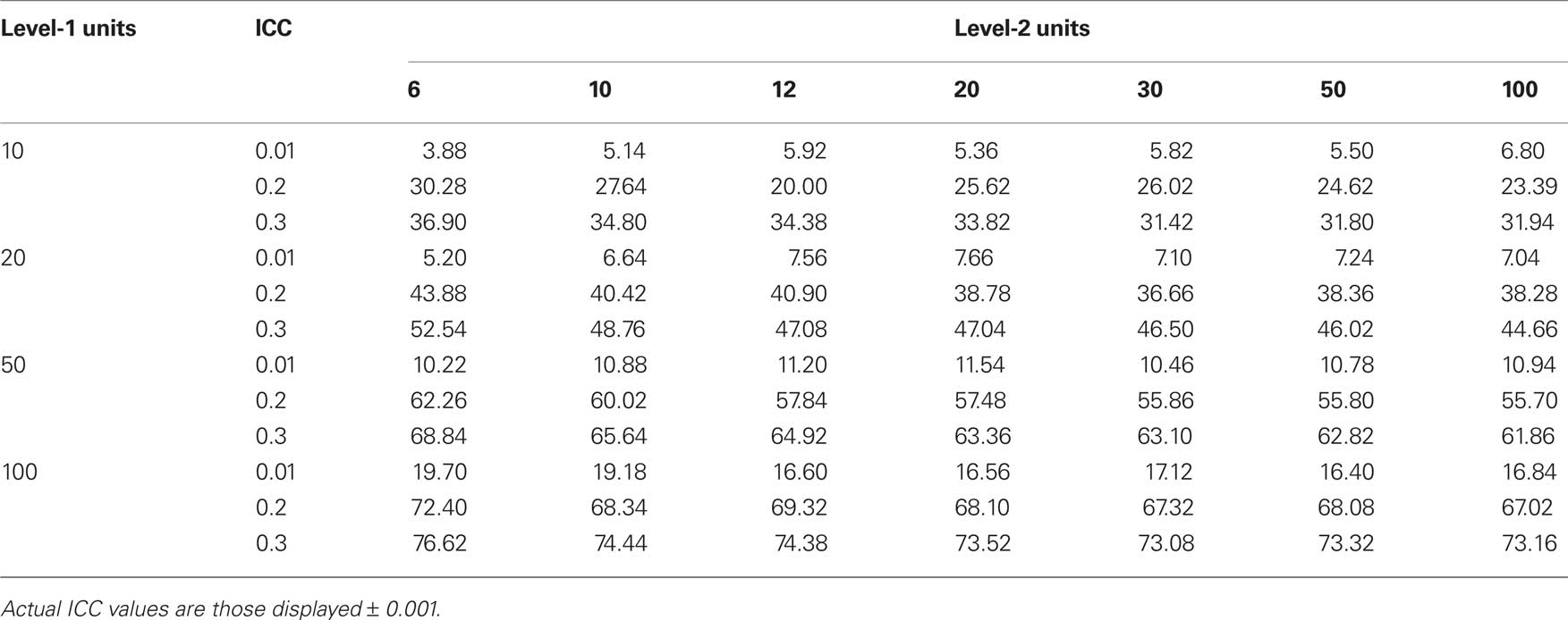
Table 1. Type-I error percentage as a function of ICC value and of the number of level-1 units (rows) and the number of level-2 units (columns).

TABLE 2

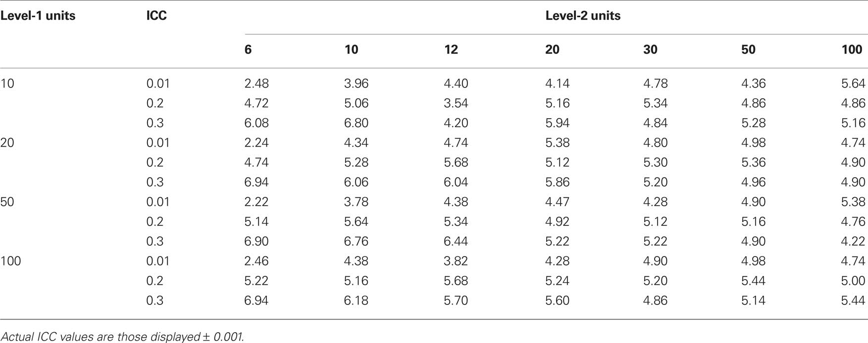
Table 2. Kish-corrected Type-I error percentage as a function of ICC value and of the number of level-1 units (rows) and the number of level-2 units (columns).

Considering the first of the examples discussed above, with 20 pupils (i.e., level-1 units) per school (level-2 units) and 30 schools (15 per learning method), in the absence of any difference between the efficiency of the two learning methods, there are 36.66% false positive results with the realistic ICC value of 0.2 (see Table 1). Considering again an ICC of 0.2, in the second example, with 50 pupils per school and 6 schools, the results are similarly worrying: a clearly unacceptable false positive rate of 62.26%. Even with the ICC value of 0.01 (considered here as a mere example of a very small non-zero value), the rate of false positive results is above 5% for both previous cases, respectively of 7.10 and 5.2%. Considering an ICC value of 0.3 (common for classroom-based clustering), the false positive rate for the sample sizes considered above is very worrying, with Type-I error rates of 46.50% and respectively 68.84%. These results make it clear how one may incorrectly conclude to a difference between conditions when in fact no such difference exists.

More generally, two main conclusions can be drawn from the results of the simulations that did not use the Kish (1965) correction. First, even with an ICC as low as 0.01, Type-I errors are always higher than 5% (except for ICC = 0.01, 6 level-2 units, and 10 level-1 units), with values well above 5% for many level-1/level-2 combinations (see Table 1). For an ICC value such as 0.2, Type-I error rates reach extremely high values, the minimum being 20% and the maximum 72.4%. With the equally plausible ICC value of 0.3, similarly worrying results are found, the minimum false positive rate being 31.42% and the maximum 76.62%. Second, the Type-I error rates increase with the number of participants per group, so that one would be better off having more groups with fewer participants per group than few groups with a lot of participants per group – note this is not an original conclusion but a well-known fact (e.g., Murray, 1998; Donner and Klar, 2000).

Considering Kish’s (1965) correction, it is clear from the results presented in Table 2 that this correction is clearly helpful, though not perfect. Indeed, while it brings the Type-I error rate down to around its nominal value (i.e., 5%), less than 50% of the cases considered here have a Type-I error rate at or below 5%. In many cases it is not conservative enough (mainly for a high number of level-1 units and for ICCs of 0.2 and 0.3 – but 0.01).

Starting from this table, one can derive the optimal number of level-1 and level-2 units that s/he should use, given the ICC that is common in her/his field. For instance, taking up again the reading method evaluation example with 20 pupils of the same grade per school and 15 schools per learning method (i.e., an intervention at the school level) and assuming an ICC of 0.2, one can read from Table 2 that applying Kish’s correction is a more or less valid solution (though slightly too liberal), since after Kish’s correction the Type-I error rate (5.30%) is just above 5%. Moreover, an examination of Table 2 shows that, having secured 30 level-2 units (and assuming the ICC is still of 0.2), one should use MLM analysis procedures because Kish’s correction does not guarantee a Type-I error rate at or below its nominal value whatever the number of level-1 units. With the second example, if only six schools (level-2 units) are available and ICC is of 0.2, Kish’s correction produces Type-I error rates below 5% if 10 or 20 level-1 units but not if more level-1 units are recruited per level-2 unit. Otherwise, if one has specific reasons for using 50 level-1 units per level-2 unit, the number of level-2 units that should be recruited in order to successfully apply Kish’ correction is 20 or 100. Again, in this latter case (i.e., 50 level-1 units per level-2 unit), MLM methods allow for analyses that often require the recruitment of a lesser and more reasonable number of level-2 units.

Conclusion

The simulation results presented here show that failing to recognize a hierarchical data structure or failing to take into account that the observations are nested under higher-order groups results in incorrect conclusions. If researchers analyze non-independent data coming from a “groups nested under treatment” design as if these data were independent, they will frequently obtain a statistically significant result, even when the treatment effect is zero. The inflation in Type-I error is more pronounced if the number of higher-order units is low, the number of lower-order of units is high, and the ICC is high. The extremely high values of Type-I errors – in some cases as high as 70% – demonstrate that non-independence of data is not just a minor problem the researchers can afford to ignore. Quite to the contrary, the present simulations suggest that researchers will most likely draw incorrect conclusions if they fail to take the non-independence into account.

Ideally, hierarchically structured data should be analyzed with MLM. In cases when multilevel modeling cannot be used because of the low number of higher-order units, one may resort to the correction method popularized by Kish (1965) because such a method is always better that resorting to pooling over level-1 units – the latter entailing the ecological fallacy, a misinterpretation of the data whereby one posits that relationships observed for groups necessarily hold for individuals (within the groups). However, simulation results presented here show that the Kish correction is not equally efficient in all cases. Assuming a perfectly balanced design (i.e., the same number of level-1 units per level-2 unit) Table 2 can be used to derive the optimal number of level-1 units that researchers should include in a study once they know the number of level-2 units that are sure to participate in the study and once they have estimated (based on previous experiments) the value of the ICC that they expect to find.

Conflict of Interest Statement

The authors declare that the research was conducted in the absence of any commercial or financial relationships that could be construed as a potential conflict of interest.

Acknowledgment

Serban C. Musca was partly supported by a research grant from the Conseil Régional d’Auvergne.

Footnotes

1. ^Mixed-effect generalized linear models refer to a general class of models that may deal with many different types of dependent variables. When the dependent variable is continuous, as in the simulations presented below, the term general (instead of generalized) is more appropriate.
2. ^See also the reference manual: http://cran.r-project.org/web/packages/arm/arm.pdf

References

Aitken, M., and Longford, N. (1986). Statistical modeling issues in school effectiveness studies. J. R. Stat. Soc. A 149, 1–43.

Bryk, A., and Raudenbush, S. W. (1992). Hierarchical Linear Models in Social and Behavioral Research: Applications and Data Analysis Methods. Newbury Park, CA: Sage Publications.

Donner, A., and Klar, N. (2000). Cluster randomization trials. Stat. Methods Med. Res. 9, 79–80.

Freedman, D. A. (2001). “Ecological inference and the ecological fallacy,” in International Encyclopedia of the Social and Behavioral Sciences, Vol. 6, eds N. J. Smelser and P. B. Baltes (Oxford: Elsevier), 4027–4030.

Gelman, A., and Hill, J. (2007). Data Analysis Using Regression and Multilevel/Hierarchical Models. Cambridge, NY: Cambridge University Press.

Goldstein, H. (1986). Multilevel mixed linear model analysis using iterative generalized least squares. Biometrika 73, 43–56.

CrossRef Full Text

Hedges, L. V., and Hedberg, E. C. (2007). Intraclass correlation values for planning group-randomized trials in education. Educ. Eval. Policy Anal. 29, 60–87.

Kenny, D. A., and Judd, C. M. (1986). Consequences of violating the independence assumption in analysis of variance. Psychol. Bull. 99, 422–431.

Kish, L. (1965). Survey Sampling. New York, NY: Wiley.

Longford, N. T. (1987). A fast scoring algorithm for maximum likelihood estimation in unbalanced mixed models with nested effects. Biometrika 74, 812–827.

CrossRef Full Text

Mason, W. M., Wong, G. Y., and Entwisle, B. (1983). “Contextual analysis through the multilevel linear model,” in Sociological Methodology 1983–1984, ed. S. Leinhardt (San Francisco: Jossey-Bass), 72–103.

McCoach, D. B., and Adelson, J. L. (2010). Dealing with dependence (part I): understanding the effects of clustered data. Gifted Child Q. 54, 152–155.

CrossRef Full Text

Murray, D. M. (1998). Design and Analysis of Group-Randomised Trials. New York, NY: Oxford University Press Inc.

R Development Core Team. (2009). R: A Language and Environment for Statistical Computing. Vienna: R Foundation for Statistical Computing.

Raudenbush, S. W., and Bryk, A. S. (2002). Hierarchical Linear Models, 2nd Edn. Thousand Oaks, CA: Sage.