Towards a pan-European coastal flood awareness system: Skill of extreme sea-level forecasts from the Copernicus Marine Service

1. Introduction

With more than 200 million European citizens – around one third of the EU population – living within 50 km from the coast, coastal flooding is one of the natural hazards with highest potential impact in Europe. Coastal flooding in Europe currently induces losses that amount to €1.4 billion per year and affects about 100,000 European citizens every year (Vousdoukas et al., 2020). With rising sea-levels and potentially exacerbated weather extremes, coastal flooding frequency is expected to increase dramatically in the coming decades (Vousdoukas et al., 2017; Oppenheimer et al., 2019). As such, increasing preparedness and response against coastal flooding becomes of outmost importance to reduce the associated risk.

Early warning systems (EWS) are a major component of disaster risk reduction (De León et al., 2006). They provide increased preparedness against upcoming natural hazards through the provision of timely information on the expected magnitude and geographic extent of the associated impacts, and they increase the response capability in the aftermath of the event. Hence, they help prevent loss of life and reduce economic impacts. Currently, while several national agencies operate country-level EWS for coastal flood risk purposes across Europe, full coverage of coastal flood early warning services across European coastlines is lacking. Besides, existing systems provide varying levels of information layers, generally lacking flood and associated impact mapping. Therefore, currently an important gap in pan-European consistent coastal flood warning information exists. Continental-scale EWS have emerged in the recent-past that demonstrate the societal relevance of seamless hazard warning information, such as the United States Geological Survey Total Water Level and Coastal Change Forecast viewer¹ and the established European Flood Awareness System², which targets pluvial and fluvial floods. In parallel to the identified existing gap for coastal flood warning information, products dedicated to the mapping, monitoring and forecasting of the coastal zone are increasingly available and developed under the European Copernicus³ program. Motivated by the identified gap, the identified opportunities within Copernicus and the associated societal relevance, a proof of concept for a pan-European early warning system for coastal flooding is under development under the H2020 project ECFAS⁴ (A proof of concept for the implementation of a European Coastal Flood Awareness System). ECFAS aims to provide information on expected flood extend, magnitude, shoreline displacement and flood impacts (population affected, projected losses, damages) induced by upcoming marine storms. ECFAS makes use of several existing Copernicus products. For its marine hazard component, it leverages on the operational ocean and wave models of the Copernicus Marine Services⁵. The pan-European, coastal sea level forecasts provided by these numerical models are used in ECFAS to feed the coastal flood models and mapping tools. For such a warning system, the ability to accurately flag and forecast coastal extreme water level events triggered by stormy conditions in a timely fashion becomes crucial. While recent studies have evaluated the skill of the Copernicus Marine Service operational models for sea-level predictions during specific storm events and coastal locations (e.g., Álvarez Fanjul et al., 2019), a pan-European assessment has not been so far performed. The objective of this manuscript is to evaluate the skill of the Copernicus Marine Service models to forecast coastal extreme sea levels during storm events and hence evaluate their suitability for coastal flood hazard forecasting applications such as ECFAS. Additionally, the evaluation outcomes are used to provide recommendations for possible future evolutions of the Copernicus Marine models towards serving such applications.

The validation provided in this study focuses on the so called coastal ‘water level’ (WL) signal, which is composed by the sterodynamic sea level (Gregory et al., 2019), astronomic tides and meteorological surges. Besides these components, water levels at the coast also experiment a contribution from waves in the form of wave setup and wave swash (Dodet et al., 2019). The explicit calculation of this contribution demands high (sub-metric) resolution and complex numerical models as well as highly accurate information of the beach geometry (e.g., nearshore bathymetry), which is currently unfeasible and unavailable yet at a pan-European scale. Widely used empirical parameterizations exist (e.g., Stockdon et al., 2006) which rely on deep water wave information. In ECFAS, the Copernicus Marine Service wave operational models will be used to compute the parameterized wave contributions. However, the lack of pan-European coastal slope information and the lack of wave contribution observations for validation makes the assessment of this contribution unfeasible. The uncertainty of the wave contributions to coastal water levels and hence flood risk at European scale is thus high. As such, the wave contributions to the total water levels at the coast are not evaluated in the current study.

This manuscript is organized as follows: first, the model and observational datasets used in this study are presented, together with the methods to process the data and intercompare them; second, the overall WL skill metrics are shown, followed by a dedicated validation of storm-driven extreme water level events and an evaluation of the impacts of the forecasting lead time on such performance metrics; third, the results are discussed and put into perspective by comparison to other regional model-studies as well as local studies that benefit from local knowledge and models and the possible implications for coastal flood hazard forecasting are outlined; finally, conclusions are drawn regarding the usability of the Copernicus Marine Service models for coastal flood awareness/forecasting applications and recommendations for future evolutions towards such applications are provided.

2. Materials and methods

2.1. Model data

European coastal WLs are retrieved from the output of the Copernicus Marine Service operational ocean forecasting systems for the European regional seas (Mediterranean Sea - MED, Black Sea-BS, Baltic Sea-BAL, Northwest Shelf -NWS, Iberian Biscay and Irish Sea -IBI, and the Arctic Sea -ARC). The coastal coverage associated to each regional model is shown in Figure 1. Northern Norway is omitted given its fjord dominated coastline, unresolved by the current models. The models resolve sea level changes due to 3D ocean circulations, steric effects, tides (except for the Black Sea-BS) and atmospheric surges due to surface atmospheric pressure and winds. Their spatial resolution ranges from 1.5 to 4.5 km and benefit from data assimilation and coupling with waves. More details on each of the regional configurations are given in Section 1 of Supplementary Materials.

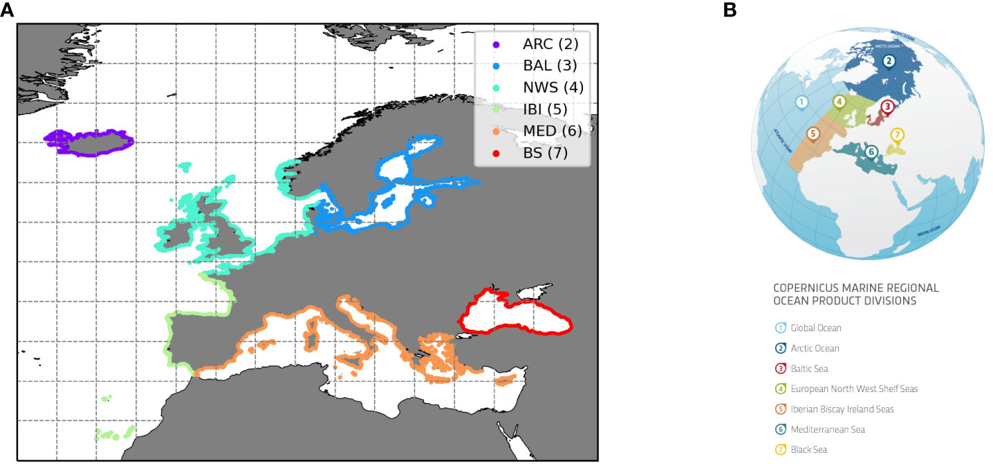
Figure 1 (A) Coastal points derived for each Copernicus Marine Service model. (B) Coverage of each Copernicus Marine Service model: 2-Arctic Ocean (ARC),3-Baltic (BAL), 4-Northwest Shelf (NWS),5-Iberian Biscay and Ireland (IBI),6-MediterraneanSea (MED),7-Black Sea(BS).

For the present validation, the model ‘best-analyses’ are used, that is, the modelling results produced for past instances in time, benefiting from data assimilation and from a model configuration at its full capacity. The target period is 2018-2020 (3 years), given the operational data availability in the Copernicus Marine Service at the time of the analysis. Best-analyses for the years 2019 and 2020 were available and hence retrieved from the service online catalogue, which corresponded to the latest release version at the time of download, namely the December 2020 version. For 2018 instead, best-analysis data is retrieved from the corresponding Copernicus Marine Service Monitoring and Forecasting Centre (MFC) archives and therefore corresponds to older -and potentially degraded - versions of the operational systems. In the present work, the coastal regions represented by the Arctic Ocean (ARC) and the Black Sea (BS) regional models are not validated due to lack of quality tide-gauge records in the target period 2018-2020. As such, these systems are omitted in this manuscript.

For evaluation of the forecast lead time impact on the coastal WL performance, ‘forecast’ data – that is, short term predictions of the non-observed future – is used. This data is also retrieved from the MFCs and again correspond to older versions of the operational systems that were active at the corresponding bulleting date. Supplementary Table 2 of Supplementary Materials summarizes the system changes that took place for each regional system during the period considered (2018-2020). Past forecast data for only three regions existed (NWS, IBI, MED). For the latter, only data from March 2020 onwards is available, so the conclusions for this region should be carefully considered. Additionally, the dataset used as reference (baseline) is specified in Supplementary Table 2 of Supplementary Materials. Ideally, the baseline should be the analysis corresponding to the bulletin date for the forecasts, that is, for the same system version, but this data was only available for the NWS region. Therefore, the baseline data for MED (Clementi et al., 2019) and IBI is the best-analysis available in Copernicus Marine at the time of this work, which corresponds to the December 2020 release.

For the Mediterranean Sea, tides are explicitly modelled since the system release in May 2021 (Clementi et al., 2021), and satisfactory tidal performance has been demonstrated in the corresponding quality information document (see Table 1 of Supplementary Materials). Since the best-analysis data collection for this validation was carried out before May 2021, the dataset for the Mediterranean Sea (MED) corresponds to the previous release version where tides were not modelled in the system. As such, tides from the thoroughly validated and widely used assimilative FES2014 global tidal model (Lyard et al., 2021) are linearly added to the Mediterranean model sea-levels in the validation. The FES2014 model resolves 34 tidal constituents, including long period tides as well as coastal overtides resulting from non-linear interactions. This linear addition entails some double counting. In FES2014, mean radiational tides at solar diurnal (S1) and solar semi-diurnal frequencies (S2) are included and these will be double counted in the WL for the MED system (Williams et al., 2018). The potential impact of non-represented non-linear interactions are discussed in section 4. Extreme WL errors induced by potential errors in the barotropic tidal solution from FES2014 are expected to be mild given the micro-tidal nature of the system, where extremes are dominated by storm-surges, except potentially in the resonant northern Adriatic Sea. All in all, tidal performance metrics are provided for each regional sea, and their contribution to extremes is also quantified.

2.2. Observation data

For validation of total water levels at the coast, tide-gauge (TG) data available in the Copernicus Marine In-situ Thematic Assembly Centre (INSTAC⁶) are used. Figure 2A shows the average time-step found in the TG records. For these 3 years, the spatial coverage is generally good except for the Eastern Mediterranean, Black Sea, Iceland, and northern Norway, for which either very little or no data is available. While hourly records prevail, temporal frequencies ranging 1-15min are observed as well as tide-gauges with multiple temporal resolutions.

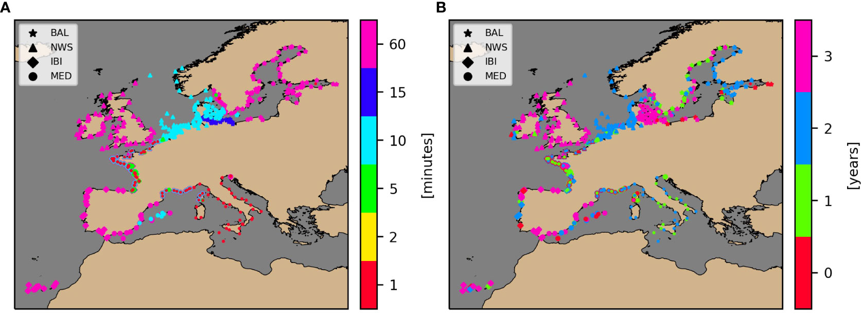
Figure 2 (A) Time-resolution of the Copernicus Marine tide-gauge network [minutes]. (B) Number of years with at least 80% data between 2018 and 2020. Marker sizes in both panels increase with time-step size in order to distinguish stations published with several different time-steps.

The number of years with at least 80% annual temporal coverage between 2018 and 2020 is given in Figure 2B. This rate is chosen to ensure the representativity of the observations as well as to allow for a robust annual tidal analysis. While Copernicus Marine tide gauge data are quality-controlled in near-real time, an additional, delayed-mode quality control procedure was applied following Perez et al. (2010); Williams et al. (2019) and visual inspection, which greatly benefited the quality of the series for extreme value assessment.

2.3. Validation procedure

In this study, the models are validated for coastal water levels as well as for their separate components (tides, non-tidal residual- NTR). In doing so, the aim is to better identify the error sources and inform the discussion about the possible modelling components that induce such errors. Observations are subjected to an hourly filtering at locations where the original time-step is below one hour (see Figure 2A). The filter applied is the widely used Pugh filter (Pugh, 1987), a filter for sea level data at intervals of 5, 10 or 15 minutes to obtain the hourly heights whilst preserving the tidal phenomena. In this way, a homogeneous hourly observational dataset across Europe is obtained. For stations with several available time-resolutions (see Figure 2A), the tide-gauge with originally largest time-step is chosen. Additionally, some tide-gauges are removed manually when located deep inside estuaries.

For the separation of WLs into tide and non-tidal residual, the Utide tidal analysis package (Codiga, 2011) is used. The modelled continuous WL timeseries (sometimes reconstructed, such as for MED) are interpolated to the non-continuous observation times, ensuring a comparable tidal signal and non-tidal residual are produced after tidal analysis. Temporal series are harmonically analysed on a yearly basis given a minimum of 80% coverage. The tidal constituents are determined using the Rayleigh criteria with a coefficient of 1 and 60 constituents. The low frequency constituents with annual and semi-annual periodicities (SA, SSA) are included in this list, and therefore seasonal modulations typically taking place at these frequencies that are triggered by non-astronomic forces (e.g., seasonal baroclinic pressures, steric heights, river discharges) are assigned to the tidal signal instead of to the non-tidal residual. As such, the non-tidal residual signal will mainly contain barotropic signals due to atmospheric pressure and wind forcing, which is commonly denoted as (storm) surge, although baroclinic signals at frequencies outside the tidal frequencies will also be present in this signal. Surge is therefore the term used hereinafter for the validation of the NTR component. Since the vertical reference datum of the tide-gauges is generally unknown, the annual bias between tide-gauges and model series is removed before computing the performance statistics.

To evaluate the general performance of WLs and its components, standard metrics are produced (centred root mean square error -cRMSE, Pearson correlation coefficient) over entire year-long time-series. These are considered to be representative of performance during average meteorological conditions. For the evaluation of extreme water level conditions, a joint water level, tide and surge performance evaluation during observed extreme events is performed. Since an exhaustive list of acknowledged, historical storm events per coastal stretch throughout Europe is not available, a methodology is developed here to detect storm-induced extreme WL events from the tide-gauge observed records between 2018 and 2020. The objective is to find extreme WL events that are simultaneously characterised by an extreme surge level, as a good indicator for stormy conditions. This type of events are henceforth denoted as ‘Extreme Events’ (EE) in this manuscript. The methodology consists in the application of a Peak over Threshold (PoT) method simultaneously on water levels and surges. A meteorological independence criteria of 3 days is used, and concurrent WL and surge extremes are searched for within 24-hour windows. Given the strong interannual variability of data availability in the tide-gauge network in 2018-2020 (Figure 2B), each year is processed using year-specific, high percentile thresholds. Given the many possible combinations of thresholds, a few iterations are carried out to achieve an annual average of 1 to 3 EEs. Finding a minimum of one extreme event would be in line with often used methods such as the annual maxima extreme value analysis method (Muis et al., 2016), and three is considered a reasonable upper limit such that focus does not deviate to milder events in the validation. The final choice is 99.9^th and 99^th annual-percentiles for WL and surges, respectively. The procedure is applied yearly for the 2018-2020 period, collecting all detected EEs per TG. An average of 3.82 EEs per TG is detected in Europe for 2018-2020 (Supplementary Figure 1 of Supplementary Materials), with above average number of EEs found in NWS and BAL. This is expected given the higher storminess characterizing these regions.

The models are hence evaluated for the list of detected EEs per TG. Metrics such as peak WL/surge error, timing error, etc are derived and averaged across the EEs per TG, with the objective to somewhat characterize average performance during storm-induced extreme events in the given period 2018-2020. Given the dependency of detected EEs on the threshold choices, and the relatively short period at hand, the performance metrics provided in this validation are to be understood as method and period specific. This aspect is further discussed in section 4.1.

Furthermore, the ability of the models to independently flag extreme events that were observed is evaluated. This represents an important characteristic for an early warning system since emergency protocols will only be activated when the models classify upcoming extreme events as ‘severe’. For this, the same percentiles employed on the observations as thresholds are applied to the model data alone. EEs independently detected in the models and in the observations are then compared. Henceforth, EEs detected from observed tide-gauge records will be denoted as ‘detected’ EEs, and those simultaneously detected from modelled results as ‘captured’ EEs. Those flagged by the model but not by the observations will be denoted as ‘false’ EEs.

Figure 3 shows an example of how the EE selection works for the tide-gauge at Galway Port, Ireland. The EE shown in Figure 3C is the only detected EE from TG observations for this year (2019) that meets the threshold criteria. The detected EE corresponds to the storm Elsa, which made landfall in Ireland around 22:00 on the 18 December 2019 and is reported to have induced a substantial storm surge and flooding (Mangan, 2019).

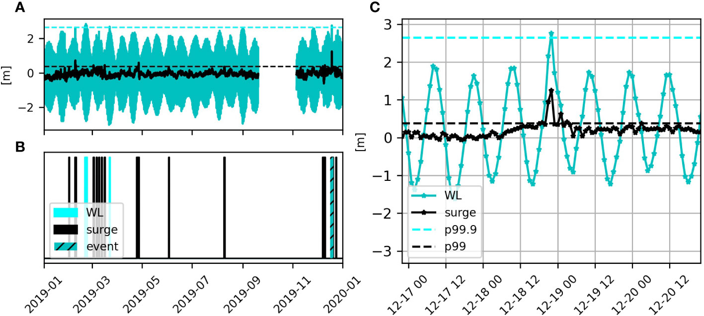
Figure 3 Example of EE detection results at the Galway Port tide-gauge, Ireland. Using the prescribed thresholds for WL (blue) and surge (black), the event detected corresponds to the passage of the storm Elsa in December 2019. (A) WL (blue) and surge(black) observed time-series and corresponding thresholds in dashed horizontal lines. (B) periods of extreme WL, surge and combined, denoting the EE. (C) Zoom of panel (A) at the detected EE.

The validation results are separated into those for the best analysis datasets (section 3.1) and for the forecasts datasets (section 3.2). For each dataset, the performance statistics under average conditions are briefly discussed first to validate the general capability of the models for coastal sea-level variability, then the focus is set on the performance during the identified EEs in tide-gauges. For average conditions, metrics are computed for 2019 given the good spatial and temporal coverage of observations, and variability of the results between 2018 and 2020 is discussed.

For the forecast dataset, the evolution of the performance statistics with an increasing forecast lead time is presented. For performance during EEs, only those EEs present in both forecast and best analysis – baseline - datasets are used. The impact of the forecast lead time is defined as the change in the performance metric for the given forecast lead time relative to the baseline.

3. Results

3.1. Validation of best analyses

Metrics for average conditions during 2019 (Table 1) show satisfactory performance for both WL and surge across regional seas, with regional-average cRMSE below 0.2m and 0.08m respectively. Correlations show above 0.9 values across regions except for the surge component in the Mediterranean (0.88).

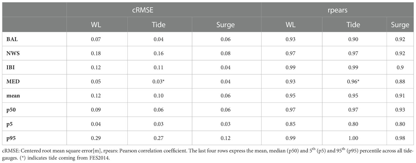
Table 1 Water-level, tide and surge performance metrics targeting average conditions for best-analyses for 2019 per regional sea.

The spatial distribution plots in Figure 4 show that the cRMSE of the WL follows the tidal error pattern, with largest errors around the North Sea (NWS), English Channel (NWS) and Irish Sea (NWS), where the tidal ranges are largest. Enhanced errors are observed around complex coastlines such as estuaries, inlets and inter-tidal areas (e.g., Wadden Sea and Halligen, south-eastern North Sea) where tides may experience local amplification and distortion. Similar effects are observed in some TGs in South-west France (Arcachon and Mimizan, IBI). Regarding the surge error, it is above average in the North Sea (NWS) and Danish Straits (BAL), which are areas characterized by high storm intensity and frequency. As shown in Table 1, correlations are high throughout the European Seas for both WL and surge, with a slightly lower value for the latter.

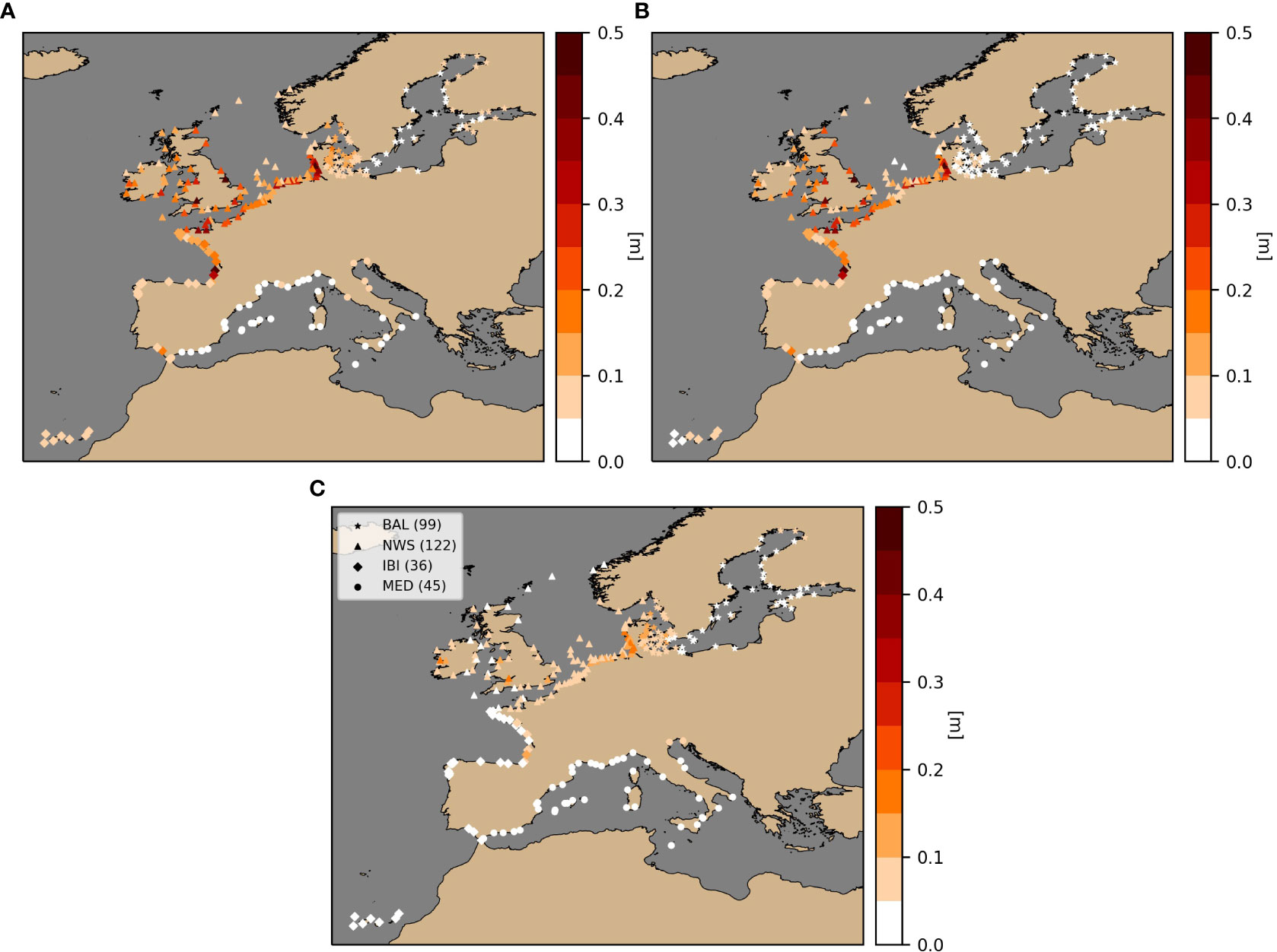
Figure 4 cRMSE for WL (A), tide (B) and surge (C) for 2019.

Regarding the variability of these metrics between 2018 and 2020, a significant improvement is noted between 2018 and 2019, while metrics are comparable between 2019 and 2020. This difference is explained by the fact that the data for 2018 corresponds to older versions of the operational systems for all regions.

3.1.1. Skills of best analyses for detected EEs

The spatial distribution of the performance statistics during the detected EEs is shown in Figure 5. Values of the metrics are available in Supplementary Table 3 of Supplementary Materials. The average error of peak modelled WLs (Figures 5A, B) for the detected EEs satisfying the selected criteria is ~-13 cm (-9.4%). Highest errors are observed in the southern North Sea (NWS) and especially for the Wadden Sea/Halligen tide-gauges, where the average (Rmean in Supplementary Table 3 of Supplementary Materials) WL peak error locally reaches -0.81 m (Husum TG, Halligen). In normalized terms (Figure 5B), the highest errors concentrate around the German Bight, Kattegat/Skagerrak (NWS) and the Mediterranean (MED).

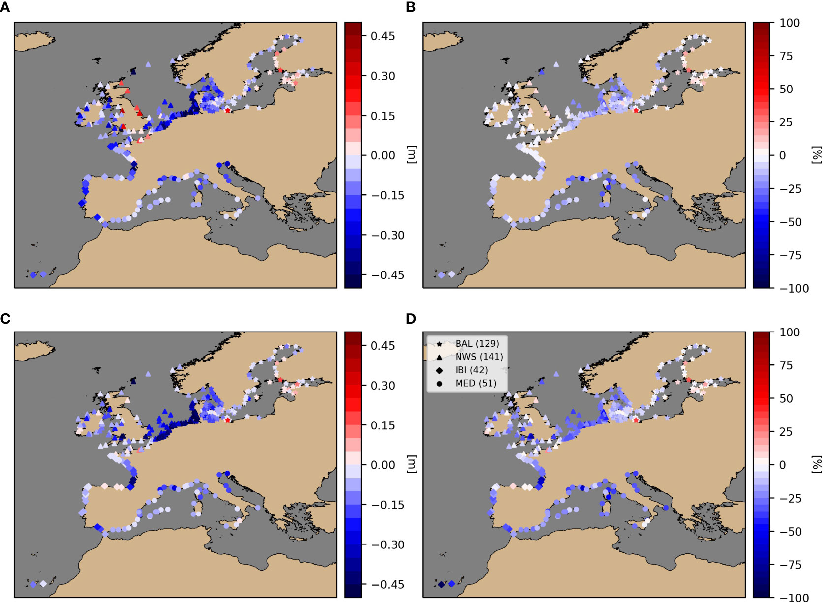
Figure 5 Average peak magnitude error ([m] (A, C) and normalized error [%] (B, D) for modelled WL (A, B) and surge (C, D) for the detected EEs based on TG observations. Regional numbers in parenthesis () in panel (D) show the number of tide-gauges within the region. Corresponding numerical values are given in Supplementary Table 3 of Supplementary Materials.

When looking at the peak surge error for the same detected EEs (Figures 5C, D), the underprediction follows the spatial distributions seen for water-level peaks but the magnitudes increase, with an average underprediction of -15 cm (-18%). As supported by literature (Horsburgh and Wilson, 2007), it has been observed that during EEs, surge peaks tend to happen a few hours before water-level maxima throughout most of North-West European tide-gauges, meaning the peak surge error shown in Figure 5 is generally higher than the surge error at the actual water-level peak time. Contrary to the peak WL error, the normalized surge peak error appears to be systematic across the domain except for the Baltic Sea. Notably, normalized peak errors can locally reach values in the order of -30%/-50% for WL and surge respectively for the largest EE recorded (R1 in Supplementary Table 3 of Supplementary Materials).

Figure 6 shows the average contribution of the tidal and surge error to the water-level peak error. On average across all tide gauge stations, surge errors dominate the total peak water-level error, contributing by 63.9%. For the two microtidal seas (BAL, MED), the contribution of the surge error dominates even more (72.5% and 79% respectively), while for the NWS the contributions are closer to evening out. In IBI instead, the tide dominates the error with a 77.2% contribution. The tide at the peak WL time appears overpredicted at places (negative contribution), compensating the generally underpredicted surge.

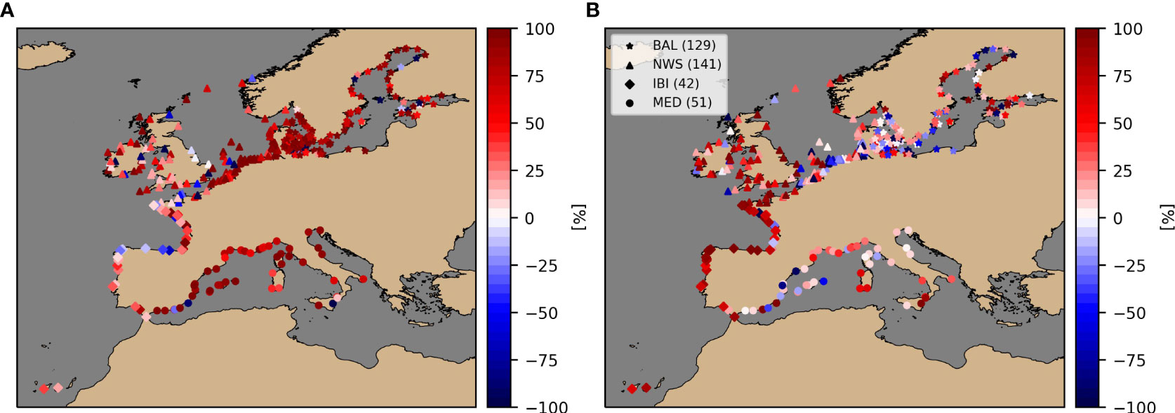
Figure 6 Average contribution [%] during the detected EEs of surge error (A) and tidal error (B) to the water-level peak magnitude error. Warm colours indicate underpredicted values, therefore positively contributing to the error.

The error in peak timing during the detected EEs appear to be generally small for WL and tides (below 1-hour, Supplementary Table 3 of Supplementary Materials), except for the Baltic Sea. Instead, larger surge peak errors are observed (order 2-3 hours). The resemblance in the spatial distribution of the peak WL and peak tide time error (not shown) in the IBI and NWS regions suggests that peak WLs coincide with tidal high waters in these regions.

3.1.2. Skills of best analyses in capturing detected EEs

The skill of the Copernicus Marine models to capture the detected observed EEs is now evaluated, independently of the skill of the exact peak representation. Figure 7 shows the percentage of captured observed EEs and falsely flagged EEs by the models. Corresponding regionally averaged numerical values are given in Supplementary Table 4 of Supplementary Materials. In average, 77% of the detected EEs are captured by the models, and 25% of the flagged EEs are false. For all regions, the percentage of captured EEs exceeds the percentage of falsely flagged EEs by a decent stretch, and remarkably so for the BAL region. Areas showing remarkably good performance - which results as a combination of a high percentage of captured EEs (dark red colours) and a low percentage of false EEs (light colours)- include northwest France and Northern Spain (IBI), the English Channel (NWS), Danish Straits and Baltic Sea as a whole (BAL), as well as Ligurian sea (MED). The North Sea (NWS) stands out as a region where the percentage of false EEs is relatively high (33%), while the percentage of captured EEs remains satisfactory (76%). This indicates that the models are able to capture the real EEs but also flag as extremes other milder events using the chosen thresholds. The latter events are not flagged as extreme in tide gauge records, indicating a wider tail for extremes in observations.

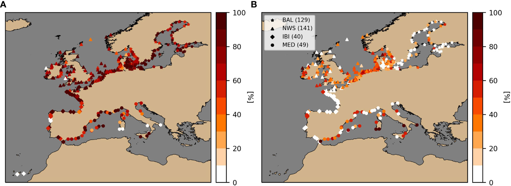
Figure 7 (A) Percentage [%] of observed detected EEs captured by models. (B) Percentage [%] of false EEs flagged by models. TG locations with 0 independently modelled EEs are not shown in panel (B) (e.g., Canary Island TGs).

In order to get a more detailed understanding of the quality of the Copernicus Marine WLs at the coast during extreme events, an analysis focusing on a number of well-known storm events between 2018 and 2020 is presented. The events and reference datasets are described in Supplementary Table 5 of Supplementary Materials. The corresponding performance metrics are given in Table 2, with Figure 8 showing the time-series at the tide-gauges used to evaluate each storm.

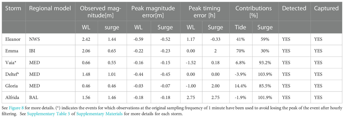
Table 2 Performance metrics of best-analyses for extreme values for a selection of storms reported to have caused coastal flooding between 2018 and 2020.

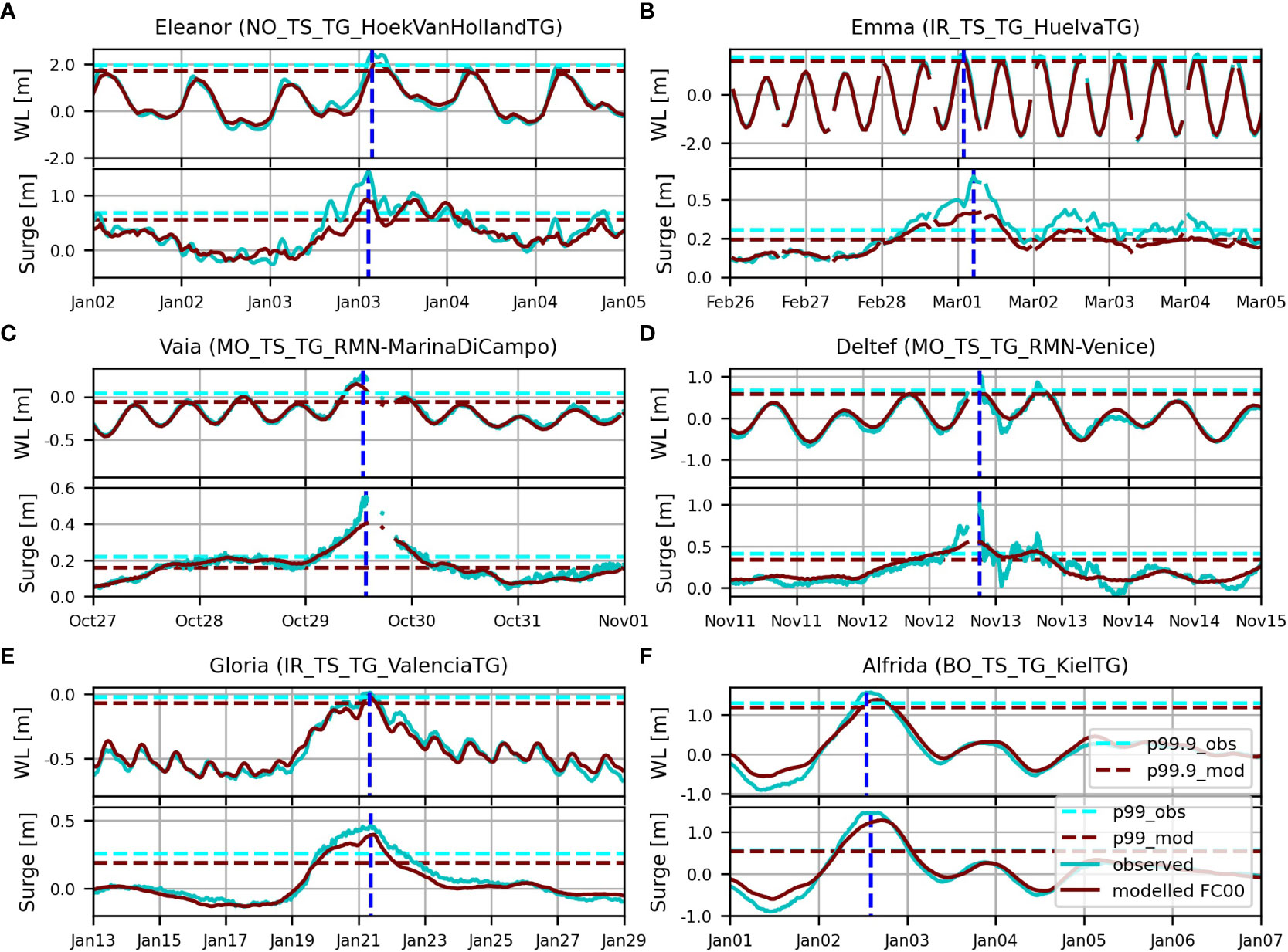
Figure 8 Water-level and surge during the list of selected events: (A)-Eleanor, 2018, Hoek Van Holland TG; (B)- Emma, 2018, Huelva TG; (C)-Vaia, 2018, Marina Di Campo TG; (D)-Detlef, 2019, Venice TG; (E)-Gloria, 2020, Valencia TG; (F)-Alfrida, 2019, Kiel TG. See Supplementary Table 5 of Supplementary Materials for more details for each storm. Blue: observed values. Red: Modelled values, best analyses (indicated as FC00). WL and surge percentile-thresholds for model and observations are shown with the corresponding colours, in horizontal dashed lines. Vertical blue line denotes the observed peak time for the plotted component. The mean sea level is that determined by the model.

The general tendency to underpredict peak water-levels and surges identified in previous sections is also evident from the time-series plots and metrics presented for the selected events. Despite the underprediction, the metrics show all EEs were flagged (captured) independently by the models. Note that for the tide-gauges at Venice (storm Detlef) and Marina Di Campo (storm Vaia), the original observations from Copernicus Marine are at 1-minute resolution and are therefore subjected to hourly-averaging (Pugh filter, see section 2.2) before computing the statistics shown in previous sections. Here however, a visual inspection of the raw observed time-series revealed that the TG data contained a few hours of missing data either right before or right after the observed water-level peak for these specific storms. This, after the Pugh hourly filter, would lead to a larger gap around the observed peak, eventually losing the observed peak for both Detlef and Vaia storms. Due to the lack of neighbouring tide-gauges to be used as an alternative, the performance metrics using the original 1-minute data sampling are included in this table (indicated by a *). Due to the presence of strong high-frequency sea-level oscillations in the 1-minute series, not captured by the Copernicus Marine models, the errors presented for these two storms are likely to be larger than those associated to hourly WL variations. Following the general observations in Figure 6, the tide error has an important contribution to the water-level peak error for storms Eleanor and Emma (NWS and IBI), while the error is clearly dominated by the surge error for the selected storms in MED and BAL. The worst performance in terms of normalized peak error (% of observed peak magnitude) is given for the storms Eleanor and Detlef, for which the peak water-level is underpredicted by -25% and -29%. For surge peak, the worst performance is given for Detlef (-45%, MED) and Eleanor (-36%, NWS) closely followed by Emma (-35%, IBI). These levels of underprediction are higher than the regional trends seen in Figure 6, specially for the latter two, which took place in 2018 (older operational systems). For Detlef (MED), the water-level error compares well to the regional average error (-21%) while the surge error is considerably larger. For this storm, as depicted by Figure 8, the water-level peak results from concurring tidal and surge peaks, suggesting the non-linear interaction between the two components could be non-negligible for this event and location, which would be missing for MED model as tides were linearly added from FES2014. Additionally, the event is characterized by a sharp and short-lived peak, while appears to be smoother in the hourly signal produced by the Copernicus Marine model. Besides the possible influence of the higher frequency signals visible in the observed 1-minute series on peak levels, literature supports that this event was induced by a small-scaled storm system that was poorly represented by the resolution of the Copernicus Marine MED atmospheric forcing (The ISMAR Team et al., 2020). Lastly, it must be noted that the TG in Venice is likely influenced by the water level exchanges with the Venice lagoon, which is not represented in the CMEMS MED model. On the other hand, the models perform notably well for the storms Gloria (MED) and Alfrida (BAL) with underpredictions of -7% and -11% respectively.

3.2. Forecasting lead time impact

For average conditions, evaluated through average annual statistics (correlation, cRMSE), WLs show no significant impact of the lead time for the 3 domains (IBI, NWS, MED). For surge instead, a considerable impact at lead times of 4 and 5 days (FC04, FC05) is observed in the NWS region, showing an increase of the centred RMSE of up to 25-30% of the observed standard deviation and a decrease of the correlation of a few to several decimal points. As anticipated, the forecast lead-time impact appears largest during extreme conditions, and therefore the following results focus on the impacts during the detected EEs.

Figures 9, 10 show the evolution of the forecast lead-time impact on performance metrics for the peak water-levels and surge levels during the detected EEs, respectively, for increasing lead times from 1 to 5 days. To convey a sense of relative importance of the impact, the metric is normalized by the observed peak value. For the water-level peak (Figure 9), no significant impact of the forecast lead time is seen for IBI while a steadily increasing impact is seen for both NWS and MED, both decaying down to an average change in the metric of around -4.5% (-1.7 cm and -10 cm). Since the baseline metric value was an underprediction, this decay indicates a further underprediction of peak water-levels with increasing forecast lead time. Box plots also get larger with increasing lead time, indicating the impact becomes larger and more widespread. At a lead time of 5 days (FC05), the strongest impacts (5^th percentile) are in the order of -3%, -9.8% and -14.8% for IBI, NWS and MED respectively (-6.8 cm, -4.5 cm and -25 cm). For surge peaks (Figure 10), the impact of forecasting lead time is more pronounced for IBI and NWS regions and remains similar to those for WL for MED, as can be expected due to its microtidal nature. At a lead time of 5 days, the average decay nears -5% (-1.6 cm) for IBI and reaches -11% (-10.6 cm) for NWS, the region that shows strongest sensitivity to the forecasting lead time. For this region, at a few coastal tide-gauges, decays in the order of -50% are seen. For the most extreme negative impacts (5^th percentile), values of -16.6%, -30.8%- and -15.1% (-5.3 cm, -33 cm and -3.7 cm) are seen for IBI, NWS and MED respectively.

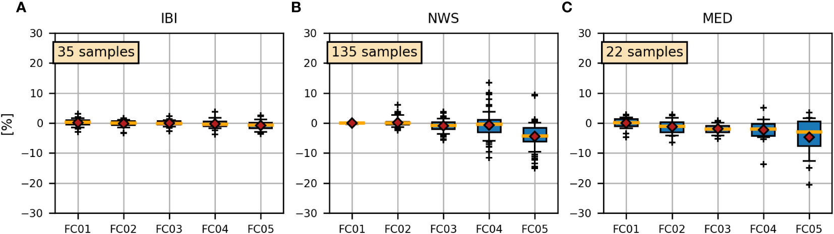
Figure 9 Evolution of the water-level peak magnitude error with the increasing forecasting lead time (1 day -FC01, 2-day -FC02,…etc), averaged over the detected EEs from observations and per region. (A)-IBI region;(B) -NWS region;(C)-MED region. Each box extends from the first (Q1) to the third (Q3) quartiles of the data, the orange line shows the median and the red diamond shows the mean value. Whiskers extend from the 5 to the 95 percentiles, and dots are outliers beyond this range.

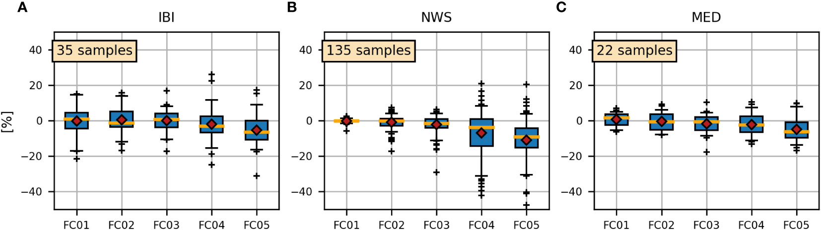
Figure 10 Evolution of the surge peak error with the increasing forecasting lead time, averaged over the detected storms from observations and per region. (A)-IBI region;(B) -NWS region;(C)-MED region. See Figure 9 for the interpretation of the whisker plot.

For both water-level and surge peaks during EEs, forecasting lead time impact leads to substantially degraded performance for lead times of 4 days and higher, and is most pronounced for the NWS region. The increased sensitivity of the surge extremes compared to the water-level extremes to forecast lead time is associated to the fact the tidal component of the water-level tends to remain relatively stable across forecasting lead times due to its gravitational (deterministic) nature.

Additionally, the evolution of the models’ skill to independently flag EEs with increasing forecast lead times is assessed. For the period covered by the forecasts, the baseline skill for flagging observed EEs for IBI, NWS and MED is of 63%, 72% and 72% respectively, and the percentage of false EEs is 14.7%, 30% and 31%. For IBI and NWS, the negative impact of the forecast lead time only becomes evident at lead times of 3 days and higher, with average detectability of EEs decaying by -17.7% for IBI and -15% for NWS for a 5-day lead time. For MED, the average values remain rather stable throughout the lead times and even show a slight improvement at forecast lead times of 2 and 4 days. The percentage of false EEs flagged by the models follows a similar but opposing trend and magnitudes, growing for increasing lead times.

While on average, the impact of the forecasting lead time on the detected extreme events remains limited (-5% and -10% for water-level and surge peaks, respectively), the range of the impacts clearly shows locations that are severely impacted, especially from lead day 4 onwards. A spatial analysis is therefore provided, with a focus on NWS as the region showing substantial and largest impacts both in absolute (>10cm) and normalized terms (>5%).

Figure 11 shows the spatial distribution of the impacts in peak water-levels in the NWS. This spatial analysis confirms that negative impacts at the highest forecasting lead times (4 and 5 days, purple and pink colours in Figure 11) dominate the picture, except for a handful of stations around the German Bight/Halligen regions and the Irish Sea which show a moderate impact early on at 2- and 3-day lead times (blue). Opposing (positive) trends are visible for a few stations around the Dutch Wadden Sea (e.g., Den Helder tide-gauge). A closer look at the data for the detected EEs in these regions reveals that some of the peaks are overpredicted at a lead time of 4 days; additionally, it is found that a few days of model forecast data are missing around the largest EE of the period for this area (early January 2019, storm Alfrida), which means that for lead times of 3 and 4 days the real peak for this storm is lost and a different peak during the storm is selected. The combination of these two effects lead to these anomalous positive trends for these stations.

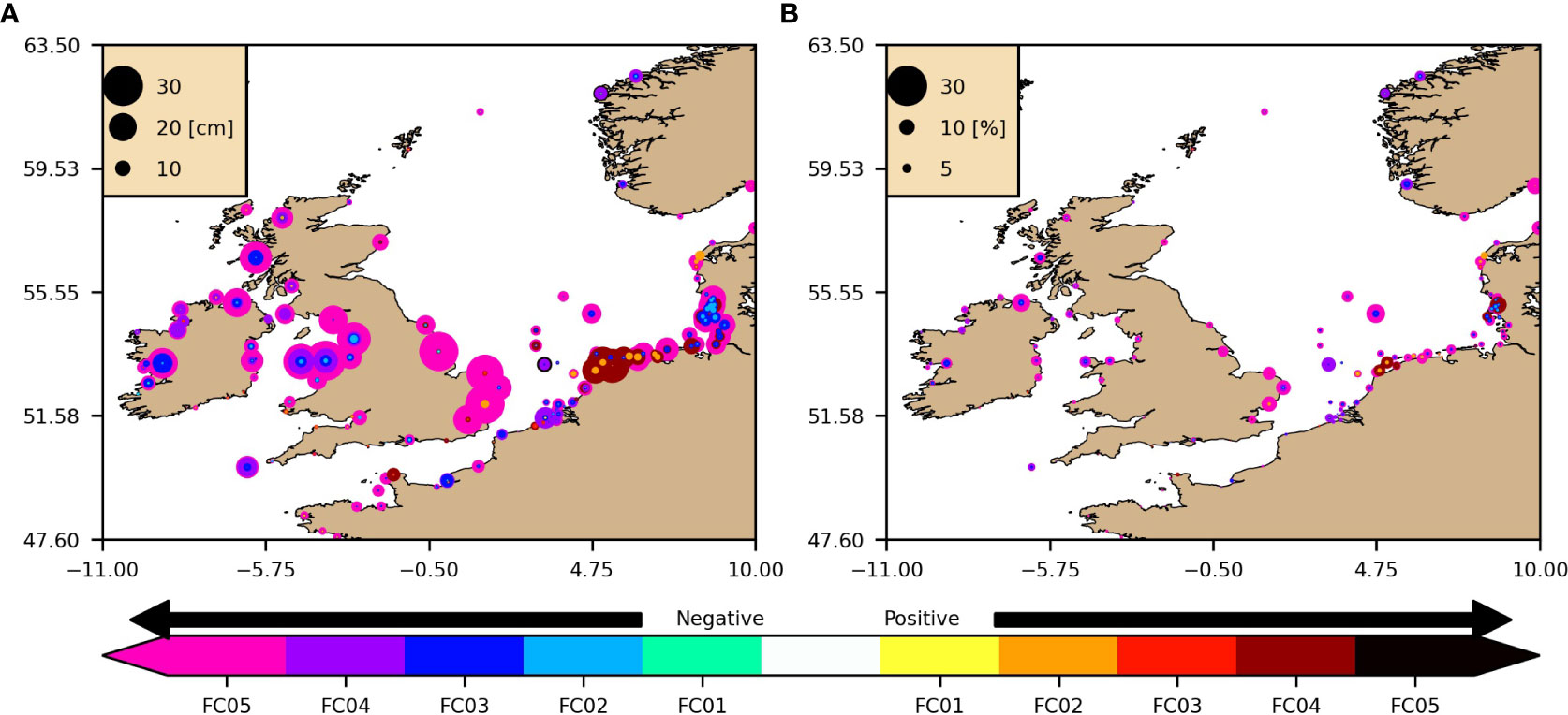
Figure 11 Relative impact of forecasting lead time from 1 to 5 days (FC01 to FC05) on the peak water-level magnitude for the detected EEs from observations. (A) –absolute scaling[cm], (B) -normalized scaling [% of observed peak magnitude]. Warm colours denote and increase of the performance metric value, cold colours denote a decrease. The forecasting lead time impact -change of the metrics relative to the baseline - is shown in the plots as concentric circles with a radius determined by the magnitude of the changes, and a colour determined by the forecasting lead time and sign of the impact (positive/negative). The lowest forecasting lead time is always plotted on top, such that one always visualizes the lowest forecasting lead time at which a substantial impact is observed.

Focusing on the impact on peak surges during the detected EEs (Figure 12), the impact of increased forecast lead time is more widespread both in magnitude and across forecasting lead times than for water-levels. In this occasion, the impact of the 4-day forecasting lead time dominates the picture in the North Sea and southern coasts of the English Channel. In the Irish Sea and Irish Atlantic coast, both lead times (4 and 5 days) show a substantial impact, and mild impacts at lead times as short as 2 days emerge at a handful of tide gauges.

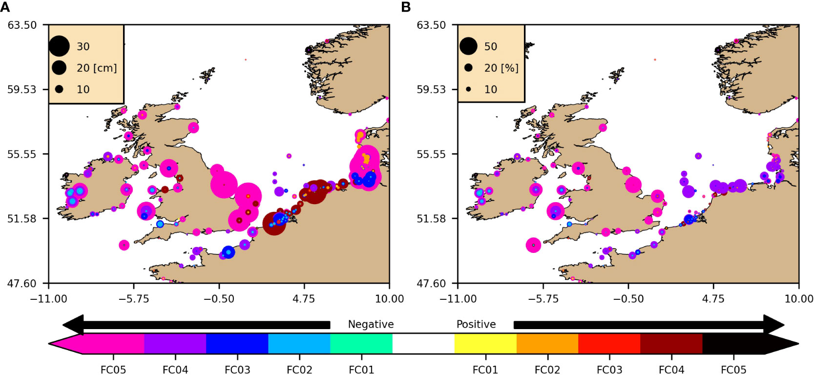
Figure 12 Relative impact of forecasting lead time from 1 to 5 days (FC01 to FC05) on the peak surge magnitude for the detected EEs from observations. (A) –absolute scaling[cm], (B) -normalized scaling [% of observed peak magnitude]. Warm colours denote an increase of the performance metric value, cold colours denote a decrease. See Figure 11 for more explanation on the plotting procedure.

4. Discussion

4.1. Limitations of the methodology

The validation results for the performance during extreme events depend on the choices made in the methodology to detect EEs, and therefore it is clearly stated that all quantitative results presented should be understood as method and period specific (2018-2020). The following choices influence the resulting list of events per TG location, and hence the resulting performance metrics. An argumentation is given for each of the choices and associated limitations, when possible:

1. The use of a simultaneous threshold for water-levels and surges: This choice is made to target extreme water-level events that were induced by extreme surge-events, and that by proxy are assumed to be induced by a passing storm. While resolved by the models, other potential triggers of extreme WLs (extreme tidal ranges (Haigh et al., 2011), interannual and inter-decadal variability of mean sea levels (Lowe et al., 2021), sea-level rise, etc) are considered out of scope.

2. Period used to define the thresholds and detect the EE: In the applied methodology, the EE detection is done on a yearly basis due to temporal coverage limitations in the tide-gauge network. This has evident shortcomings. First, it forces the algorithm to find extreme water-level and surge conditions (while not simultaneously) every year and at all locations. While this is not unrealistic for most regions (and widely accepted by the research community in the field when using, for example, the annual maxima method for extreme WL value distributions, where a maximum is selected every year (Muis et al., 2016)), such approach somewhat neglects the potential for strong interannual variability in the frequency and intensity of storms at each location. Second, the period at hand (3 years) might contain a handful of extreme events but it is considered short for a robust extreme value analysis, which generally relies on multidecadal records. Therefore, even if the right EEs were detected with the algorithm, the list of EEs within 2018-2020 might not be representative of the local historical extreme conditions.

3. Selection of thresholds to define an extreme event: The use of a peak-over-threshold methodology (PoT) to isolate extreme events is common practice in coastal flood risk assessments. The percentile used as threshold varies between studies (e.g., 98^th or 99^th percentile, see Kirezci et al., 2020 and Oppenheimer et al., 2019 respectively), to which results are inevitably sensitive.

Regarding the limitation number 3, Supplementary Figure 2 of Supplementary Materials shows the sensitivity of the average WL and surge peak errors to the threshold selection for several combinations of water level and surge thresholds. For water level peak errors, the results for the different threshold options generally fall within the range of errors provided in this analysis both in absolute and normalized scaling terms. For surges, results show a larger sensitivity. As expected, out-of-range errors are found for those options with higher surge thresholds, which target fewer and more extreme surge events. For events determined purely by surge extremes (option 4 in Supplementary Figure 2 of Supplementary Materials), the surge peak appears to be larger than in those events determined by both water-level and surge, and therefore lead to larger underpredictions. Indeed, some of the largest surge peaks took place during lower tidal levels and therefore didn’t trigger an extreme water level. The implications of this larger surge error under realistic, high tide conditions cannot be assessed given the short record length at hand. In general, the range of errors for the different options are well within the error range shown for the largest events (R1 in Supplementary Table 3 of Supplementary Materials) for the chosen set of thresholds. Using only water level thresholds (options 1 and 3 Supplementary Figure 2 of Supplementary Materials) leads to an increased number of events per year (from 2-4 to 7-10 for tidally dominated regions), many of which are characterized by high tides and small surges, leading to comparatively smaller errors and therefore biasing the assessment towards more optimistic results. These results showcase the usefulness of the simultaneous threshold method on water level and surge components when targeting performance under stormy conditions. Indeed, the error metrics derived for known, hand-picked past extreme events (Table 2) are within the error ranges derived from the extreme event methodology. While informative for the given period and tide-gauge locations, the current results cannot be strictly extrapolated in time and space. In terms of spatial coverage, important gaps exist for the Eastern Mediterranean, Black Sea and Iceland (Arctic) regions given the lack of high-quality tide-gauge records in the Copernicus Marine Service. In terms of temporal coverage, the limitations are mostly associated to the model data coverage. All in all, the order of magnitude and spatial distribution of the errors given in this analysis provide a useful overview of the expected performance for Copernicus Marine Service models for extreme coastal water levels during storms.

4.2. Benchmarking and model configuration impacts

Overall, best analyses of WL produced by the Copernicus Marine Service regional monitoring and forecasting systems show satisfactory comparisons to TG data. However, peak water levels tend to be underestimated. In general, the model performance during average conditions is comparable to other state-of-the-art models with similar spatial resolutions and dedicatedly designed for coastal flood hazard applications at regional scales. In comparison to the European scale 2D model for storm surges by Fernández-Montblanc et al., 2020b, the models show overall comparable skill while substantially better metrics (RMSE, correlation) for Copernicus Marine Service models in the Mediterranean and Baltic Sea. This can be explained by the fact that baroclinic (3D) motions not present in 2D barotropic models contribute greatly in these micro-tidal regions to the water level variability and its extremes (Fernández-Montblanc et al., 2020a; Woodworth et al., 2021). Fernández-Montblanc et al., 2020b also report generally underpredicted extreme surges throughout European coastlines, with maximum errors comparable to the ones presented in this validation (several decimeters). At a regional scale, a handful of models are found in literature that outperform the Copernicus Marine Service operational models for water levels at the coast. This is especially the case for northern Europe, where a vast expertise and long history in numerical modelling for coastal safety purposes exists (De Goede, 2020). In a qualitative level, the better skills for WLs found in northern European systems can generally be explained by a higher resolution of the hydrodynamic models (Andrée et al., 2021), higher resolution of the atmospheric forcing (Brüning et al., 2014), and/or a dedicated calibration targeting coastal water level representation (Zijl et al., 2013). The latter demonstrates not only the benefits of increased model resolution but also the high sensitivity of a 2D barotropic model to bathymetry and bottom friction. Such sensitivity simultaneously poses a great improvement potential through calibration and the potentially great impact that uncertainties in these terms can have in modelled water levels in shelf regions. In Copernicus Marine Service models, no dedicated spatial calibration is performed for these terms, because the models do not specifically target coastal water levels but rather aim to represent the full, 3-dimensional ocean physical field (temperature, salinity, currents…) across all relevant temporal and spatial scales. For other regions of Europe such as the Mediterranean (MED) and the Iberian Biscay (IBI), the performance of the models found in literature is more comparable to the skills reported for the Copernicus Marine Service models. In comparison to the IBI model, errors reported in literature are in the order of several decimeters for individual storms and are mostly attributed to an underprediction of the wind-setup component of the surge (Pasquet et al., 2014; Fortunato et al., 2016; De Alfonso et al., 2020). Interestingly, some of these studies shows that the level of underprediction can vary significantly for different settings of the wind drag coefficient. Indeed, the drag coefficient has been demonstrated to be sea-state dependent in numerous studies and as such it forms part of the components that are usually exchanged in ocean-wave coupled models (e.g., Chune and Aouf, 2018). This topic deserves a dedicated discussion and is addressed further on in this section. For the Mediterranean region, several semi-regional to local forecasting models exists, especially so for the Adriatic Sea region. The range of peak error values shown in this study is representative of that found in multi-resolution, multi-model approaches in the region (Ferrarin et al., 2020). Notably, systems that target much higher spatial resolutions (decametric coastal resolution, kilometric atmospheric resolution) demonstrate the resulting improved extreme water-level skills (Ferrarin et al., 2019).

Despite the coarser coastal resolution of the Copernicus Marine Service models compared to the benchmarking studies presented, it is noteworthy that most studies report some level of underprediction, which points to a common limitation for all models. This is likely related to inaccuracies in the atmospheric forcing, which strongly determine the extreme water level performance. Indeed, at regional scales, atmospheric forcing models operated at the resolution of ~10km (e.g., the European Centre for Medium-Range Weather Forecasts Integrated Forecast System -ECMWF IFS- product used by most Copernicus Marine Service models) often lack the spatial resolution needed to resolve local wind regimes and may therefore underestimate extreme winds at the coast. This was the case for storm Detlef in Venice in November 2019 (see Table 2), where the MED atmospheric model forcing underestimated peak winds by up to 20 m/s, as shown by Giesen et al., 2021. They report that local small-scaled interactions such as orographic steering often play a role in the development of such Mediterranean marine storms, which would require higher resolution atmospheric models. Such small scales also characterize the development and maintenance of Mediterranean hurricanes - Medicanes (Flaounas et al., 2022), which can trigger severe coastal flooding (Androulidakis et al., 2022). In a different environment such as the Irish Sea, Bricheno et al. (2013) demonstrate the substantial sensitivity of wave and storm surge heights during stormy conditions when increasing the atmospheric forcing resolution from 12 km to 4 km. Besides the benefit of added atmospheric resolution, another conclusion stemming from this benchmarking exercise is that local, coastal refinement of ocean models can also greatly enhance their coastal WL performance, especially around shallow coastal regions characterized by fine scale geometry (e.g., islands, coastal lagoon and bay areas, large shallow estuaries and fjord areas). Indeed, WLs can experience very local effects in these environments (Wang et al., 2012; Jacob and Stanev, 2021). The effects are generally related to local tidal distortions (evident under average meteorological conditions) or local enhancement of the storm-surges (evident under extreme meteorological conditions, Bloemendaal et al., 2019). The higher coastal resolutions found in existing operational systems is often achieved by either a computationally lighter, purely barotropic setup (2D) or by the inclusion of nested coastal models or local zooms (Declerck et al., 2016) in regional models, which allow for feasible computational times in operational forecasting. Nevertheless, local effects aside, current kilometric model resolutions seem to suffice to satisfactorily capture WLs across most European coasts, as highlighted by the good model WL skill seen under average to severe conditions. In the vast majority of the coastal stretches, the largest part of the WL error during extreme conditions is still expected to be attributed to the error in atmospheric forcing or specific model settings affecting the surge generation, not resolution. It is highlighted that wave contributions to the coastal total water level (wave setup, wave runup), not considered in our assessment, would undoubtedly greatly benefit from higher local resolutions, given the smaller spatial scales of the wave processes compared to tides, surges and sterodynamic sea-levels.

Beyond the effects of the atmospheric forcing and model resolution, other modelling components and features might be impacting the performance during storms. Notably, the implementation of wetting and drying could strongly influence the performance of the models in shallow water regions such as the Wadden Sea and German Bight (southern North Sea, NWS), as demonstrated by O’Dea et al. (2020). These are the regions where the models currently perform worst. For estuarine areas where local hydrodynamics are the result of interacting ocean and riverine forcing (Spicer et al., 2019), performance will remain a challenge in such large-scale models that mostly rely on climatology (Durand et al., 2019). Furthermore, the bathymetry employed by the Copernicus Marine Service models (see Supplementary Table 1 of Supplementary Materials) is generally outdated (before 2016). Updated datasets of the EMODnet bathymetry offer higher resolution and accuracy, as well as a better representation of intertidal bathymetry which may greatly improve the modelling capabilities at the coast. More accurate bathymetry could substantially improve tidal performance (Wang et al., 2021; Blakely et al., 2022) in the IBI and the NWS models, where tides induce an important part of the errors seen for both average and extreme WL conditions.

Some physical processes and parameterizations potentially impacting water-levels are also identified. In the current operational Copernicus Marine Service models, the models account for the wave coupling effects at different levels (Supplementary Table 1 of Supplementary Materials). The IBI and NWS models offer the most complete coupling, while BAL and MED models only account for the Stokes Drift and the wave drag effects respectively and could therefore be limiting the water-level representation capabilities of these models. Several recent studies have reported on the significant impact of the wave coupling on water-levels around the European Northwest Shelf and Baltic regions, in particular during extreme events, which may increase coastal extreme sea-levels by several decimeters (Staneva et al., 2016; Staneva et al., 2017; Lewis et al., 2019; Bonaduce et al., 2020; Staneva et al., 2021).These studies argue that, on the shelf, the strongest impact is induced by the sea-state dependent sea-surface roughness, which can be importantly enhanced during growing, young sea states (Bertin et al., 2015, Pineau-Guillou et al., 2020). This process is currently lacking in the BAL model. Other coupling components (stokes-drift and mixing related), while less dominant, may enhance peak water-levels locally by 10-20% (Staneva et al., 2016). Given the reported strong impact of wave to ocean coupling, the extreme sea-level skill of the ocean models at hand may rely not only on the level of ocean-wave coupling, but notably on the accuracy of their wave-model counterparts through wave-surge interactions. Furthermore, the choice of wind stress parameterization often differs between the wave and ocean models, with wave models assuming neutral wind conditions whilst ocean models accounting for the stability of the atmospheric boundary layer. Clementi et al. (2017) reported substantially increased extreme wave heights when coupling ocean and wave models for this process. These enhanced wave extremes could feedback on the water-levels through the aforementioned interaction processes. Moreover, the atmospheric model used to force the ocean and wave models –ECMWF IFS for most models - also adopts its own parameterization for the wind stress, in this case determined by the sea-state of the wave model to which it is coupled, influencing the resulting surface winds and stress. As shown by Pineau-Guillou et al. (2018), wave-dependent surface drag values for the ECMWF operational model may be over-estimated for high winds, leading to underestimated 10-meter winds compared to in-situ observations. Importantly, the 10-meter wind needs translating to wind stress before used to force the ocean and wave models. Isolating the (underestimated) 10-meter winds from the associated (overestimated) drag would in principle result in biased (underpredicted) wind stresses that force the ocean and wave models. In summary, inconsistencies on the wind stress formulation between ocean and wave models, but also with the atmospheric model forcing them, may partly explain the systematic underprediction of extreme sea-levels in the models. Additionally lacking complex feedback processes within the marine atmospheric boundary layer (Lemarié et al., 2021) could be further affecting the representation of water-levels. So far, impacts have been studied in the context of ocean mesoscale representation and are still to be explored for coastal locations and under energetic conditions during storms.

For the MED system, it is noteworthy that the model results used in this validation do not include the dynamic representation of tides, and therefore miss non-linear effects between tides and other components. These have been reported to be small in the Mediterranean in some studies (Marcos et al., 2009) and non-negligible in others (Ferrarin et al., 2013). All in all, tides are explicitly represented in the MED operational system since May 2021 and these non-linear effects are therefore currently captured. Another component potentially influencing the water level performance at the coast is the assimilation of altimetric sea levels. The assimilation of this information varies across regions. For MED and NWS, sea level anomaly (SLA) is assimilated in deep waters only, owing to the increasing inaccuracy of altimetry towards the coast (e.g., land contamination) but also of the geophysical correction terms used to filter the signal. For IBI, SLA is assimilated at all depths and could therefore be experimenting induced detriments close to the coast. While the benefits of altimetry assimilation are undeniable in deep waters, the suitability of the employed datasets and configurations for the representation of coastal water levels is still to be explored. Furthermore, temporal smoothing effects might be playing a role in the performance of the water levels in the Copernicus Marine Service models. The ocean models provide outputs that vary between hourly-mean (IBI, MED) and hourly-instantaneous (NWS, BAL). Most models (IBI, NWS, MED) have recently included in their catalogue 15-minute instantaneous surface fields, including sea-levels, but of too short temporal coverage (2021 onwards) to be used in this analysis. A preliminary analysis of the 15-minute series for a short one-month period shows increased high percentiles for IBI, presumably due to a better representation of the tidal high waters. For the MED, while hourly-mean outputs are provided, negligible impacts on the tidal representation are expected due to its micro-tidal regime. Instead, it is found that the hourly-filtering used on the high-frequency Mediterranean TG data (see Figure 2A) leads to the filtering of high-frequency sea-level oscillations (HFSLO, e.g., seiches, meteo-tsunamis) and thus leads to the attenuation of the observed water-level variability. These HFSLO have been identified in several tide-gauges and, despite representing processes that are out of the current scope of the regional ocean models at hand, their potential impact on extremes and thus coastal flood risk is undeniable (Šepić et al., 2015, Pérez-Gómez et al., 2021). Meteo-tsunamis can notably constitute a strong coastal hazard in micro-tidal areas such as the Mediterranean and Black Sea (Vilibić et al., 2021). An overview of the impact of the hourly filtering in the performance statistics during extremes is provided in Supplementary Figure 3 of Supplementary Materials, showing that hourly-filtering leads to reduced peak magnitude errors due to attenuated observed peak water-levels in the Mediterranean. The potential to include these high-frequency motions in the Copernicus Marine Service models needs further research and development. In this context, the residual presence of HFSLO processes and others like wave-setup in the hourly-filtered sea-level observations from tide-gauges cannot be discarded (Woodworth et al., 2019), which would penalize the model performance as these processes are currently not resolved in the models.

Regarding the capability of the Copernicus Marine Service models to independently flag extreme events, a satisfactory score is achieved for all regions, with a hit rate of >70% for all but for the MED region (64%). Besides, an above-average rate of false EEs is seen for the NWS and MED regions. For the MED, the results for both captured and false rates could be attributed to a combination of the relatively low extreme threshold magnitude compared to the standard variability range (the difference in magnitude between extremes and normal amplitudes being smaller than for other regions), and the underpredicted extremes in the model which make this difference even smaller.

4.3. Forecast skill impact

The assessment of the forecast lead time impact on the coastal water level skill shows limited impact under average conditions. Surges show a stronger skill decay than water levels, and most evident at a lead time of four days and longer. The sensitivity to the forecasting lead time is also most evident during the detected extreme events, due to the increased contribution of the storm surge component, and for the NWS region where storm surges are largest. This is expected as a result of the forecast skills and uncertainties inherited from the driving meteorological forcing. In the Copernicus Marine Service systems, the meteorological forcing is an external boundary condition and therefore has a pre-determined accuracy. While the results show limited impact in average up to 4 days of forecasting lead time, which is considered suitable for coastal flood risk warning systems, some locations are identified where impacts emerge at lower lead times. Notably, the available period for the evaluation of the forecasting lead time impact is short, given the scarcity of past forecast data available, which limits the conclusions derived. This is particularly true for the Mediterranean model, for which only 10 months of forecast water level data is available, and the Baltic model for which forecast archives simply don’t exist. In this region though, important impacts could be expected given the large contribution of the surge to the water level variability and the high level of storminess of the region.

4.4. Recommendations and future perspectives

The performance metrics during storm-induced extreme events and the stability of the performance up to a lead time of 4 days demonstrate the suitability of the Copernicus Marine Service systems for pan-European coastal flood early awareness applications such as ECFAS. While the results presented provide a valuable overview of the expected performance of the Copernicus Marine operational models for coastal extreme water-level representation, the short temporal availability of model data and the use of a non-homogeneous model dataset, spanning multiple release versions of the systems, limited the characterisation of the extreme coastal WL skill. In the future, upon availability of homogeneous multi-decadal modelled records, robust extreme value analyses could be performed, and a better characterization of the forecast lead time impact could be achieved if past forecasts were routinely stored.

The systematic underprediction of extreme water levels is potentially attributed to inaccurate atmospheric forcing forecasts by comparison to other studies using higher atmospheric resolution and/or local atmospheric products. While the accuracy of the atmospheric forecast products used to force the Copernicus Marine Service models is pre-determined (while under continuous development by the responsible agencies), ensemble forecasts could greatly reduce the associated uncertainty on the coastal water level forecasts and contribute to their probabilistic forecasting. The level to which the errors in meteorological forcing are responsible for the errors on the modelled surges still needs to be thoroughly evaluated, in order to discern externally introduced errors from possible model-inherent sources for the misrepresentation and be able to direct model development efforts accordingly. In this study, a list of model developments is identified for the potential improvement of the coastal water levels. Updated background bathymetric datasets are recommended across regional models based on ongoing initiatives that aim for increased accuracy, resolution, and coastal coverage bathymetric datasets (e.g., EMODnet bathymetry⁷, GEBCO⁸, Seabed 2030⁹), which could notably improve tidal propagation and the generation of surge during stormy conditions. In terms of tidal representation, efforts should be directed to the improvement of this deterministic component notably in the IBI and NWS systems, where a large part of the error is attributed to the tide. Higher spatial resolution together with a wetting and drying scheme would greatly improve the capabilities of the ocean models around complex shallow coastal areas and estuarine/intertidal areas such as the Wadden Sea or German Bight, where the highest performance errors are currently found. Small scaled, local non-linear effects on WLs around geometrically complex coastlines remain a challenge for these regional models, posing the need for locally nested high resolution coastal models to resolve them. In that respect, the Copernicus Marine Service operational models provide an ideal baseline on which to nest local models, given the kilometric scale, high quality, and data-assimilation supported information of the 3D ocean field they provide across European seas. In this regard, emerging dedicated coastal altimetry datasets (Benveniste et al., 2020) pose the potential to improve model skill at the coast through assimilation, and to improve validation at ungauged coastal locations. Further wave-coupling could help improve the surge performance during storms and would increase the harmonisation between the regional products and thus of the pan-European forecasts. Besides, a consistency evaluation of the wind stress as computed by the atmospheric, wave and ocean models involved in the water-level forecasts is recommended, given its dominant role on the generation of surge. More broadly, missing ocean-atmospheric coupling effects on the coastal water level performance remain to be thoroughly assessed. For the Mediterranean region, the presence of observed high frequency sea-level oscillations (e.g. meteo-tsunamis) and the implications for coastal extremes are highlighted, and the level to which the regional-scale model can capture these processes needs further investigation. Recently emerging, quality-controlled minute-resolution tide-gauge record databases pose the opportunity to further explore these aspects (Zemunik et al., 2022). Besides the physics needed to capture such events, the production of minute-resolution forecasts would certainly pose a challenge in terms of operability of the forecasts.

In relation to these recommended evolution activities, it should be kept in mind that to remain state-of-the-art, Copernicus Marine forecasting systems are continuously evolving and will continue to do so during Copernicus 2 (2021-2027), with several of the evolution activities recommended here already planned (e.g., Melet et al., 2021). The physical content of the numerical models underpinning the forecasts of water level will evolve with more processes being included, the systems will be further coupled (ocean-wave systems), more observations will be assimilated to better constrain the systems including in coastal zones, the spatial resolution will be increased, wetting and drying will be implemented in different regions, outputs will be provided at higher frequencies, etc. The publication of past forecasts and the potential for ensemble-based probabilistic forecasting is also envisioned. Therefore, the skills of the forecasting systems will evolve with future new releases of the Copernicus Marine Service portfolios, and so will the capability of the systems to support coastal flood awareness and warning systems.

In conclusion, the Copernicus Marine Service models provide valuable marine hazard information for broad-scale coastal flood awareness applications such as ECFAS, where the objective is to provide currently lacking pan- European information on coastal flood warnings with sufficient local relevance. In order to target coastal areas characterized by fine scale water level and wave dynamics, higher resolution local systems could be nested as downstream components of the parent pan-European system, which could rely on the warnings raised by the parent model for activation. Nested configurations could refine marine hazard and hence flood forecasts locally where needed, while benefiting from the ECFAS coverage and functionalities. The ECFAS system, supported by the Copernicus Marine Service models for operational marine forcing, poses an excellent opportunity for such downstream applications.

Data availability statement

Copernicus Marine Service data is openly available through the service website. Past forecasts were kindly provided by the corresponding Marine and Forecasting Centres and are not publicly available. Requests to access these datasets should be directed to https://www.ecfas.eu/contact-us/.

Author contributions

MIA contributed to the research conceptualization and wrote the full manuscript, contributed to algorithm writing and data analysis. AM supervised and provided guidance for all the activities. CA contributed to manuscript revision, read, and approved the submitted version

Funding

This work has received funding from the ECFAS project (a proof-of-concept for the implementation of a European Copernicus Coastal Flood Awareness System) funded by the European Union’s Horizon 2020 research and innovation programme under grant agreement No. 101004211.

Acknowledgments

The authors thank the regional Monitoring and Forecasting Centers (MFC) of the Copernicus Marine Service for providing data for both past forecasts and best analyses not available in the Copernicus Marine Service portal. The authors especially thank Stefania Ciliberti (Euro-Mediterranean Center on Climate Change, CMCC), Vibeke Huess (Danish Meteorological Institute, DMI), Laura Tuomi (Finish Meteorological Institute, FMI), Marcos García Sotillo (Puertos del Estado), Arancha Amo Baladrón (Nologin consulting), Emanuela Clementi (Euro-Mediterranean Center on Climate Change, CMCC), Marina Tonani (UK Met Office affiliation at the time of data receival, currently affiliated at Mercator Ocean International),Isabella Ascione (UK Met Office), Andrew Saulter (UK Met Office), Gerasimos Korres (Hellenic Centre for Marine Research,HCMR), Arild Burud(Norwegian Meteorological Institute) and Laurent Bertino (Nansen Environmental and Remote Sensing Center, NERSC) for their dedicated efforts to retrieve the data and their expert advice on its use. The authors also thank Enrico Duo (IUSS Pavia) for his review of early versions on the manuscript, and Juan Montes Perez (University of Cadiz) for his critical review of the final manuscript.

Conflict of interest

The authors declare that the research was conducted in the absence of any commercial or financial relationships that could be construed as a potential conflict of interest.

Publisher’s note

All claims expressed in this article are solely those of the authors and do not necessarily represent those of their affiliated organizations, or those of the publisher, the editors and the reviewers. Any product that may be evaluated in this article, or claim that may be made by its manufacturer, is not guaranteed or endorsed by the publisher.

Supplementary material

The Supplementary Material for this article can be found online at: https://www.frontiersin.org/articles/10.3389/fmars.2022.1091844/full#supplementary-material

Footnotes

1. ^ https://www.usgs.gov/centers/spcmsc/science/operational-total-water-level-and-coastal-change-forecasts.
2. ^ https://www.efas.eu/en.
3. ^ https://www.copernicus.eu/en.
4. ^ https://www.ecfas.eu.
5. ^ https://marine.copernicus.eu.
6. ^ http://www.marineinsitu.eu/).
7. ^ https://emodnet.ec.europa.eu/en/bathymetry.
8. ^ https://www.gebco.net/.
9. ^ https://seabed2030.org/.

References

Álvarez Fanjul E., de Pascual Collar A., Pérez Gómez B., De Alfonso M., García Sotillo M., Staneva J., et al. (2019). “Sea Level, sea surface temperature and SWH extreme percentiles: combined analysis from model results and in situ observations,” in Copernicus Marine service ocean state report, issue 3, J. Oper. Oceanogr. vol. 12 (sup1), 31–39. doi: 10.1080/1755876X.2019.1633075
Andrée E., Su J., Larsen M. A. D., Madsen K. S., Drews M. (2021). Simulating major storm surge events in a complex coastal region. Ocean Modelling 162, 101802. doi: 10.1016/j.ocemod.2021.101802
Androulidakis Y., Makris C., Mallios Z., Pytharoulis I., Baltikas V., Krestenitis Y. (2022). Storm surges during a medicane in the ionian sea. In Editor Tzovara E HCMR. Marine and Inland Waters Research Symposium 2022 Proceedings. Porto Heli, Argolida, Greece, 16–19. doi: 10.21203/rs.3.rs-1781884/v1
Benveniste J., Birol F., Calafat F., Cazenave A., Dieng H., Gouzenes Y., et al. (2020). Coastal sea level anomalies and associated trends from Jason satellite altimetry over 2002-2018. Sci. Data 7, 357. doi: 10.1038/s41597-020-00694-w
Bertin X., Li K., Roland A., Bidlot J. R. (2015). The contribution of short-waves in storm surges: Two case studies in the bay of Biscay. Continental Shelf Res. 96, 1–15. doi: 10.1016/j.csr.2015.01.005
Blakely C., Ling G., Pringle W. J., Contreras M. T., Wirasaet D., Westerink J., et al. (2022). Dissipation and bathymetric sensitivities in an unstructured mesh global tidal model. J. Geophysical Research: Oceans 127, e2021JC018178. doi: 10.1029/2021JC018178
Bloemendaal N., Muis S., Haarsma R. J., Verlaan M., Irazoqui Apecechea M., de Moel H., et al. (2019). Global modeling of tropical cyclone storm surges using high-resolution forecasts. Clim Dyn 52, 5031–5044. doi: 10.1007/s00382-018-4430-x
Bonaduce A., Staneva J., Grayek S., Bidlot J. R., Breivik Ø. (2020). Sea-State contributions to sea-level variability in the European seas. Ocean Dynamics 70 (12), 1547–1569. doi: 10.1007/s10236-020-01404-1
Bricheno L. M., Soret A., Wolf J., Jorba O., Baldasano J. M.. (2013). Effect of High-Resolution Meteorological Forcing on Nearshore Wave and Current Model Performance. J Atmos Ocean Technol 30 (6), 1021–1037. doi: 10.1175/JTECH-D-12-00087.1
Brüning T., Janssen F., Kleine E., Komo H., Maßmann S., Menzenhauer-Schumacher I., et al. (2014). Operational ocean forecasting for German coastal waters. Modelling 81, 273–290. Available at: https://hdl.handle.net/20.500.11970/101695.
Chune S. L., Aouf L. (2018). Wave effects in global ocean modeling: parametrizations vs. forcing from a wave model. Ocean Dynamics 68 (12), 1739–1758. doi: 10.1007/s10236-018-1220-2
Clementi E., Aydogdu A., Goglio A. C., Pistoia J., Escudier R., Drudi, et al. (2021). Mediterranean Sea Analysis and forecast (CMEMS MED-currents, EAS6 system) (Version 1) (Copernicus Monitoring Environment Marine Service (CMEMS). Avalable at: https://data.marine.copernicus.eu/product/MEDSEA_ANALYSISFORECAST_PHY_006_013/description?view=-&product_id=-&option=-.
Clementi E., Oddo P., Drudi M., Pinardi N., Korres G., Grandi A. (2017). Coupling hydrodynamic and wave models: first step and sensitivity experiments in the Mediterranean Sea. Ocean Dynamics 67, 1293–1312. doi: 10.1007/s10236-017-1087-7
Clementi E., Pistoia J., Escudier R., Delrosso D., Drudi M., Grandi A., et al. (2019). Mediterranean Sea Analysis and forecast (CMEMS MED-currents EAS5 system 2017-2020) (Copernicus Monitoring Environment Marine Service (CMEMS). Avalable at: https://www.cmcc.it/doi/mediterranean-sea-physics-analysis-andforecast-cmems-med-currents-eas5-system.
Codiga D. L. (2011). Unified tidal analysis and prediction using the UTide Matlab functions. Technical Report 2011-01. Graduate School of Oceanography, University of Rhode Island, Narragansett, RI. 59pp. doi: 10.13140/RG.2.1.3761.2008
De Alfonso M., María García-Valdecasas J., Aznar R., Pérez-Gómez B., Rodríguez P., Javier de los Santos F., et al. (2020). “Record wave storm in the gulf of cadiz over the past 20 years and its impact on harbours,” in Copernicus Marine service ocean state report, issue 4, J. Oper. Oceanogr. vol. 13 (sup1), 137–144. doi: 10.1080/1755876X.2020.1785097
Declerck A., Ourmières Y., Molcard A. (2016). Assessment of the coastal dynamics in a nested zoom and feedback on the boundary current: the north-Western Mediterranean Sea case. Ocean Dynamics 66, 1529–1542. doi: 10.1007/s10236-016-0985-4
De Goede E. D. (2020). Historical overview of 2D and 3D hydrodynamic modelling of shallow water flows in the Netherlands. Ocean Dynamics 70 (4), 521–539. doi: 10.1007/s10236-019-01336-5
De León J. C. V., Bogardi J., Dannenmann S., Basher R. (2006). Early warning systems in the context of disaster risk management. Entwicklung Ländlicher Raum 2, 23–25. Available at: https://collections.unu.edu/eserv/UNU:2837/ELR_dt_23-25.pdf.
Dodet G., Melet A., Ardhuin F., Bertin X., Idier D., Almar R. (2019). The contribution of wind generated waves to coastal sea level changes. Surveys Geophysics 40, 1562–1601. doi: 10.1007/s10712-019-09557-5
Durand F., Piecuch C. G., Becker M., Papa F., Raju S. V., Khan J. U., et al. (2019). Impact of continental freshwater runoff on coastal sea level. Surveys Geophysics 40 (6), 1437–1466. doi: 10.1007/s10712-019-09536-w
Fernández-Montblanc T., Gómez-Enri J., Ciavola P. (2020a). The role of mean Sea level annual cycle on extreme water levels along European coastline. Remote Sens. 12 (20), 3419. doi: 10.3390/rs12203419
Fernández-Montblanc T., Vousdoukas M. I., Mentaschi L., Ciavola P. (2020b). A pan-European high resolution storm surge hindcast. Environ. Int. 135, 105367. doi: 10.1016/j.envint.2019.105367
Ferrarin C., Davolio S., Bellafiore D., Ghezzo M., Maicu F., Mc Kiver W., et al. (2019). Cross-scale operational oceanography in the Adriatic Sea. J. Operational Oceanography 12 (2), 86–103. doi: 10.1080/1755876X.2019.1576275
Ferrarin C., Valentini A., Vodopivec M., Klaric D., Massaro G., Bajo M., et al. (2020). Integrated sea storm management strategy: the 29 October 2018 event in the Adriatic Sea. Natural Hazards Earth System Sci. 20 (1), 73–93. doi: 10.5194/nhess-20-73-2020
Ferrarin C., Roland A., Bajo M., Umgiesser G., Cucco A., Davolio S., et al. (2013). Tidesurge-wave modelling and forecasting in the Mediterranean Sea with focus on the Italian coast. Ocean Modelling 61, 38–48. doi: 10.1016/j.ocemod.2012.10.003
Flaounas E., Davolio S., Raveh-Rubin S., Pantillon F., Miglietta M. M., Gaertner M. A., et al. (2022). Mediterranean Cyclones: Current knowledge and open questions on dynamics, prediction, climatology and impacts. Weather Climate Dynamics 3 (1), 173–208. doi: 10.5194/wcd-3-173-2022
Fortunato A. B., Li K., Bertin X., Rodrigues M., Miguez B. M. (2016). Determination of extreme sea levels along the Iberian Atlantic coast. Ocean Eng. 111, 471–482. doi: 10.1016/j.oceaneng.2015.11.031
Giesen R., Clementi E., Bajo M., Federico I., Stoffelen A., Santoleri R. (2021). “The November 2019 record high water levels in Venice, Italy,” in Copernicus Marine service ocean state report, issue 5, J. Oper. Oceanogr. vol. 14 (sup1), 156–162. doi: 10.1080/1755876X.2021.1946240
Gregory J. M., Griffies S. M., Hughes C. W., Lowe J. A., Church J. A., Fukimori I., et al. (2019). Concepts and terminology for Sea level: Mean, variability and change, both local and global. Survey Geophysics 40, 1251–1289. doi: 10.1007/s10712-019-09525-z
Haigh I. D., Eliot M., Pattiaratchi C. (2011). Global influences of the 18.61 year nodal cycle and 8.85 year cycle of lunar perigee on high tidal levels. J. Geophysical Research: Oceans 116 (C6), C06025. doi: 10.1029/2010JC006645
Horsburgh K. J., Wilson C. (2007). Tide-surge interaction and its role in the distribution of surge residuals in the north Sea. J. Geophysical Research: Oceans 112 (C8), C08003. doi: 10.1029/2006JC004033
Jacob B., Stanev E. V. (2021). Understanding the impact of bathymetric changes in the German bight on coastal hydrodynamics: One step toward realistic morphodynamic modeling. Front. Mar. Sci. 8, 576. doi: 10.5194/egusphere-egu21-15453
Kirezci E., Young I. R., Ranasinghe R., Muis S., Nicholls R. J., Lincke D., et al. (2020). Projections of global-scale extreme sea levels and resulting episodic coastal flooding over the 21st century. Sci. Rep. 10 (1), 1–12. doi: 10.1038/s41598-020-67736-6
Lemarié F., Samson G., Redelsperger J. L., Giordani H., Brivoal T., Madec G. (2021). A simplified atmospheric boundary layer model for an improved representation of air–sea interactions in eddying oceanic models: implementation and first evaluation in NEMO (4.0). Geoscientific Model. Dev. 14 (1), 543–572. doi: 10.5194/gmd-14-543-2021
Lewis H. W., Castillo Sanchez J. M., Siddorn J., King R. R., Tonani M., Saulter A., et al. (2019). Can wave coupling improve operational regional ocean forecasts for the north-west European shelf? Ocean Sci. 15 (3), 669–690. doi: 10.5194/os-15-669-2019
Lowe R. J., Cuttler M. V., Hansen J. E. (2021). Climatic drivers of extreme sea level events along the coastline of Western Australia. Earth's Future 9 (4), e2020EF001620. doi: 10.1029/2020EF001620
Lyard F. H., Allain D. J., Cancet M., Carrère L., Picot N. (2021). FES2014 global ocean tide atlas: design and performance. Ocean Sci. 17 (3), 615–649. doi: 10.5194/os-17-615-2021
Mangan I. (2019). West Of Ireland battered after storm Elsa brings ferocious winds and flooding (The Irish Mirror). Available at: https://www.irishmirror.ie/weather/storm-elsa-galway-weather-flooding-21129364.
Marcos M., Tsimplis M. N., Shaw A. G. P. (2009). Sea level extremes in southern Europe. J. Geophys. Res. 114, C01007. doi: 10.1029/2008JC004912
Melet A., Buontempo C., Mattiuzzi M., Salomon P., Bahurel P., Breyannis G., et al. (2021). European Copernicus Services to inform on sea-level rise adaptation: current status and perspectives. Front. Mar. Sci 8, 703425. doi: 10.3389/fmars.2021.703425
Muis S., Verlaan M., Winsemius H. C., Aerts J. C., Ward P. J. (2016). A global reanalysis of storm surges and extreme sea levels. Nat. Commun. 7 (1), 1–12. doi: 10.1038/ncomms11969
O’Dea E., Bell M. J., Coward A., Holt J.. (2020). Implementation and assessment of a fluxlimiter based wetting and drying scheme in NEMO. Ocean Modelling 155, 101708. doi: 10.1016/j.ocemod.2020.101708
Oppenheimer M., Glavovic B. C., Hinkel J., van de Wal R., Magnan A. K., Abd-Elgawad A. (2019). “Sea Level rise and implications for low-lying islands, coasts and communities,” in IPCC special report on the ocean and cryosphere in a changing climate. Eds. Pörtner H.-O., Roberts D. C., Masson-Delmotte V., Zhai P., Tignor M., Poloczanska E., Mintenbeck K., Alegría A., Nicolai M., Okem A., Petzold J., Rama B., Weyer N. M. (Cambridge, UK and New York, NY, USA: Cambridge University Press), 321–445. doi: 10.1017/9781009157964.006
Pasquet A., Michaud H., Aouf L., Baraille R., Bru C., Correard, et al. (2014). Implémentation d'un nouveau modèle opérationnel de prévision des vagues et surcotes marines. XIIIèmes Journées Nationales Génie Côtier–Génie Civil 2014 (13), 149–158. doi: 10.5150/jngcgc.2014.017
Perez B., De Alfonso Alonso-Muñoyerro M., Huess V., Rickards L. (2010). Near real time quality control and validation of Sea level in-situ data within MyOcean. Technical report MYO-INS-SL_QC. Avalable at: https://archimer.ifremer.fr/doc/00631/74307/73931.pdf.
Pérez-Gómez B., García-León M., García-Valdecasas J., Clementi E., Aranda C. M., Pérez-Rubio S., et al. (2021). Understanding sea level processes during Western Mediterranean storm Gloria. Front. Mar. Sci 8, 647437. doi: 10.3389/fmars.2021.647437
Pineau-Guillou L., Ardhuin F., Bouin M. N., Redelsperger J. L., Chapron B., Bidlot J. R., et al. (2018). Strong winds in a coupled wave–atmosphere model during a north Atlantic storm event: Evaluation against observations. Q. J. R. Meteorological Soc. 144 (711), 317–332. doi: 10.1002/qj.3205
Pineau-Guillou L., Bouin M. N., Ardhuin F., Lyard F., Bidlot J. R., Chapron B., et al. (2020). Impact of wave-dependent stress on storm surge simulations in the North Sea: Ocean model evaluation against in situ and satellite observations. Ocean Modelling 154, 101694. doi: 10.1016/j.ocemod.2020.101694
Pugh D. T. (1987). “Tides, surges and mean Sea level,” in A handbook for engineers and scientists (Chichester: John Wiley & Sons), 472.
Spicer P., Huguenard K., Ross L., Rickard L. N. (2019). High-frequency tide-Surge-River interaction in estuaries: Causes and implications for coastal flooding. J. Geophysical Research: Oceans 124 (12), 9517–9530. doi: 10.1029/2019JC015466
Staneva J., Alari V., Breivik Ø., Bidlot J. R., Mogensen K. (2017). Effects of wave-induced forcing on a circulation model of the north Sea. Ocean Dynamics 67 (1), 81–101. doi: 10.1007/s10236-016-1009-0
Staneva J., Grayek S., Behrens A., Günther H. (2021). GCOAST: skill assessments of coupling wave and circulation models (NEMO-WAM). J. Phys. Conf. Ser. 1730, 12071. doi: 10.1088/1742-6596/1730/1/012071
Staneva J., Wahle K., Koch W., Behrens A., Fenoglio-Marc L., Stanev E. V. (2016). Coastal flooding: impact of waves on storm surge during extremes–a case study for the German bight. Natural Hazards Earth System Sci. 16 (11), 2373–2389. doi: 10.5194/nhess-16-2373-2016
Stockdon H. F., Holman R. A., Howd P. A., Sallenger A. H. Jr. (2006). Empirical parameterization of setup, swash, and runup. Coast. Eng. 53, 573–588. doi: 10.1016/j.coastaleng.2005.12.005
Šepić J., Vilibić I., Lafon A., Macheboeuf L., Ivanović Z.. (2015). High-frequency sea level oscillations in the Mediterranean and their connection to synoptic patterns. Progress in Oceanography 137, 284–298. doi: 10.1016/j.pocean.2015.07.005
The ISMAR Team, Cavaleri L., Bajo M., Barbariol F., Bastianini M., Benetazzo A., et al. (2020). The 2019 flooding of Venice and its implications for future predictions. Oceanography 33 (1), 42–49. doi: 10.5670/oceanog.2020.105
Vilibić I., Denamiel C., Zemunik P., Monserrat S.. (2021). The Mediterranean and black Sea meteotsunamis: an overview. Nat. Hazards 106, 1223–1267. doi: 10.1007/s11069-020-04306-z
Vousdoukas M. I., Mentaschi L., Hinkel J., Ward P. J., Mongelli I., Ciscar J. C., et al. (2020). Economic motivation for raising coastal flood defenses in Europe. Nat. Commun. 11 (1), 1–11. doi: 10.1038/s41467-020-15665-3
Vousdoukas M. I., Mentaschi L., Voukouvalas E., Verlaan M., Feyen L. (2017). Extreme sea levels on the rise along europe's coasts. Earth's Future 5 (3), 304–323. doi: 10.1002/2016EF000505
Wang Z. B., Hoekstra P., Burchard H., Ridderinkhof H., De Swart H. E., Stive M. J. F. (2012). Morphodynamics of the wadden Sea and its barrier island system. Ocean Coast. Manage. 68, 39–57. doi: 10.1016/j.ocecoaman.2011.12.022
Wang X., Verlaan M., Apecechea M. I., Lin H. X. (2021). Computation-efficient parameter estimation for a high-resolution global tide and surge model. J. Geophysical Research: Oceans 126 (3), e2020JC016917. doi: 10.1029/2020JC016917
Williams J., Irazoqui Apecechea M., Saulter A., Horsburgh K. J. (2018). Radiational tides: their double-counting in storm surge forecasts and contribution to the highest astronomical tide. Ocean Sci. 14 (5), 1057–1068. doi: 10.5194/os-14-1057-2018
Williams J., Matthews A., Jevrejeva S. (2019). “Development of an automatic tide gauge processing system,” in National oceanography centre research and consultancy report, 64 (Southampton: National Oceanography Centre), 26.
Woodworth P. L., Hunter J. R., Marcos M., Hughes C. W. (2021). Towards reliable global allowances for sea level rise. Global Planetary Change 203, 103522. doi: 10.1016/j.gloplacha.2021.103522
Woodworth P. L., Melet A., Marcos M., Ray R. D., Wöppelmann G., Sasaki Y. N., et al. (2019). Forcing factors affecting sea level changes at the coast. Surveys Geophysics 40, 1351–1397. doi: 10.1007/s10712-019-09531-1
Zemunik P., Denamiel C., Šepić J., Vilibić I. (2022). High-frequency sea-level analysis: Global distributions. Global Planetary Change 210, 103775. doi: 10.1016/j.gloplacha.2022.103775
Keywords: early warning, coastal flooding, sea-level extremes, storm-surges, Copernicus Marine Service
Citation: Irazoqui Apecechea M, Melet A and Armaroli C (2023) Towards a pan-European coastal flood awareness system: Skill of extreme sea-level forecasts from the Copernicus Marine Service. Front. Mar. Sci. 9:1091844. doi: 10.3389/fmars.2022.1091844
Received: 07 November 2022; Accepted: 13 December 2022;
Published: 19 January 2023.
Edited by:
Alejandro Jose Souza, Center for Research and Advanced Studies - Mérida Unit, MexicoReviewed by:
Marta Rodrigues, National Laboratory for Civil Engineering, PortugalIvica Janekovic, University of Western Australia, Australia
Copyright © 2023 Irazoqui Apecechea, Melet and Armaroli. This is an open-access article distributed under the terms of the Creative Commons Attribution License (CC BY). The use, distribution or reproduction in other forums is permitted, provided the original author(s) and the copyright owner(s) are credited and that the original publication in this journal is cited, in accordance with accepted academic practice. No use, distribution or reproduction is permitted which does not comply with these terms.
*Correspondence: Maialen Irazoqui Apecechea, mirazoki@mercator-ocean.fr