Mapping the Intertidal Microphytobenthos Gross Primary Production Part I: Coupling Multispectral Remote Sensing and Physical Modeling
 Vona Méléder1*
  Raphael Savelli2
  Alexandre Barnett1,2
  Pierre Polsenaere3
  Pierre Gernez1
  Philippe Cugier4 Astrid Lerouxel1 Anthony Le Bris1,5 Christine Dupuy2
  Vincent Le Fouest2
  Johann Lavaud2,6
- 1Mer Molécules Santé (EA 21 60), Université de Nantes, Nantes, France
- 2LIENSs ‘Littoral ENvironnement et Sociétés’ UMR 7266, Institut du Littoral et de l’Environnement, CNRS/Université de La Rochelle, La Rochelle, France
- 3Laboratoire Environnement Ressources des Pertuis Charentais (LER-PC), Ifremer, L’Houmeau, France
- 4Département Dynamiques de l’Environnement Côtier, Laboratoire d’Ecologie Benthique, Ifremer, Plouzané, France
- 5Centre d’Etude et de Valorisation des Algues (CEVA), Pleubian, France
- 6Takuvik Joint International Laboratory UMI3376, CNRS (France) & ULaval (Canada), Département de Biologie, Université Laval, Québec, QC, Canada
The gross primary production (GPP) of intertidal mudflat microphytobenthos supports important ecosystem services such as shoreline stabilization and food production, and it contributes to blue carbon. However, monitoring microphytobenthos GPP over a long-term and large spatial scale is rendered difficult by its high temporal and spatial variability. To overcome this issue, we developed an algorithm to map microphytobenthos GPP in which the following are coupled: (i) NDVI maps derived from high spatial resolution satellite images (SPOT6 or Pléiades), estimating the horizontal distribution of the microphytobenthos biomass; (ii) emersion time, photosynthetically active radiation (PAR), and mud surface temperature simulated from the physical model MARS-3D; (iii) photophysiological parameters retrieved from Production–irradiance (P–E) curves, obtained under controlled conditions of PAR and temperature, using benthic chambers, and expressing the production rate into mg C h–1 m–2 ndvi–1. The productivity was directly calibrated to NDVI to be consistent with remote-sensing measurements of microphytobenthos biomass and was spatially upscaled using satellite-derived NDVI maps acquired at different seasons. The remotely sensed microphytobenthos GPP reasonably compared with in situ GPP measurements. It was highest in March with a daily production reaching 50.2 mg C m–2 d–1, and lowest in July with a daily production of 22.3 mg C m–2 d–1. Our remote sensing algorithm is a new step in the perspective of mapping microphytobenthos GPP over large mudflats to estimate its actual contribution to ecosystem functions, including blue carbon, from local and global scales.
Introduction
Tidal mudflats are soft sediment coastal marine ecosystems that undergo regular tidal inundation. Their bare surface is colonized by biofilms constituted of photosynthetic microorganisms (microalgae and cyanobacteria), collectively known as microphytobenthos (MPB) (e.g., MacIntyre et al., 1996; Paterson and Hagerthey, 2001). Under temperate latitudes, MPB assemblages are mainly dominated by diatoms that form a brown dense biofilm at the sediment surface during daytime low tides (MacIntyre et al., 1996; Underwood and Kromkamp, 1999). Intertidal flats provide important ecosystem services such as biodiversity depositories, storm protection, and shoreline stabilization (Murray et al., 2018; Legge et al., 2020). They also provide essential food resource for higher trophic levels, from benthic fauna to birds (Herman et al., 2000; Kang et al., 2006; Jardine et al., 2015), and for pelagic organisms when MPB is resuspended in the water column (Perissinotto et al., 2003; Krumme et al., 2008). As such, they contribute to the so-called blue carbon (Otani and Endo, 2019; Legge et al., 2020). With sand and rocky flats, tidal mudflats are one of the most extensive coastal ecosystems, with a recent global area estimation of at least 127,921 km2 (Murray et al., 2018). With a global annual gross primary production (GPP) estimated to be in the order of 0.5 Gt C y–1 (Cahoon, 1999), MPB are of key importance for local and global coastal ecosystem functions, including carbon budget. However, their actual contribution remains unknown, due to the lack of estimation at ecosystem scale (i.e., the entire mudflat). A more comprehensive mapping of these intertidal mudflats is therefore needed to improve the accuracy of coastal carbon budgets (Legge et al., 2020).
The spatial heterogeneity of intertidal mudflats, as well as the high degree of temporal variability in process rates, adds to the challenges of accurately quantifying carbon stocks and flows in coastal areas (Legge et al., 2020). MPB spatiotemporal distribution is highly variable, as it is driven by highly variable physical [photosynthetically active radiation (PAR), mud surface temperature (MST), tides, and waves] and biological (grazing, biostabilization, and bioturbation) factors (e.g., Pinckney and Zingmark, 1991; Kingston, 2002; Cohn et al., 2003; Consalvey et al., 2004; Spilmont et al., 2007; Coelho et al., 2009, 2011; Serôdio et al., 2012; Savelli et al., 2018). Such a variability impedes on an accurate and robust assessment of MPB contribution to the coastal and global marine carbon cycle. To assess MPB biomass and/or GPP, tidal mudflat measurements are usually limited to single-point sampling (e.g., Vieira et al., 2013; Orvain et al., 2014; Cartaxana et al., 2015; Pniewski et al., 2015). Station-based sampling makes it possible to locally assess MPB temporal dynamics, but it fails to describe MPB spatial and temporal variations at the scale of the entire mudflat (Forster and Kromkamp, 2006). Whereas only few studies have resolved MPB variability using sampling campaigns requiring time and important logistical resources (i.e., Guarini et al., 1998; Ubertini et al., 2012), satellite remote sensing appears to be the most efficient upscaling tool. Since the end of the last century, starting with Jobson et al. (1980) initiative, airborne and spaceborne remote sensing methods have been developing increasingly and are now more widely used for MPB studies (Méléder et al., 2003b; van der Wal et al., 2010; Brito et al., 2013; Benyoucef et al., 2014; Echappé et al., 2018). Remote sensing data can cover large spatial scales (from one meter to several kilometers), and vegetation indices such as the normalized difference vegetation index (NDVI) were successfully applied to multispectral broadband satellite sensors to map MPB biomass at the scale of a whole mudflat (e.g., Méléder et al., 2003b; van der Wal et al., 2010; Brito et al., 2013; Benyoucef et al., 2014; Echappé et al., 2018). However, although it is common use to estimate terrestrial vegetation GPP (e.g., Goetz et al., 1999; Huemmrich et al., 2010) and oceanic GPP (e.g., Babin et al., 2015) from space, remote sensing has never been used to map MPB GPP over an entire mudflat before the study by Daggers et al. (2018). While this recent study represents a major contribution to the field, their GPP model does not take into account the seasonal variability of photophysiology (Kromkamp and Forster, 2006) and also strongly depends on the relationship between NDVI and sediment MPB chlorophyll-a (Chl a) concentration, which is known to be highly sensitive to Chl a sampling depth, MPB vertical distribution, and MPB small-scale horizontal variability (Jesus et al., 2006). In order to resolve the NDVI versus Chl a issue, we propose here an original method where GPP is directly calibrated to NDVI. First, a GPP algorithm was obtained using laboratory measurements of NDVI and carbon fluxes (mg C h–1 m–2) fitted on Production–Irradiance (P–E) curves. Second, the seasonal variability of the photophysiological parameters was taken into account in a series of laboratory experiments performed during winter, spring, and summer. Third, the NDVI-calibrated GPP algorithm was applied to high-resolution satellite images acquired during the three seasons and coupled to emersion time, mud surface temperature (MST), and light intensity (PAR) obtained from the physical model for Applications at Regional Scale (MARS-3D). Finally, we compared the remotely sensed GPP with field observations, and we discussed the ability of our algorithm to map MPB GPP at mudflat scale and to provide new insights on the role of MPB in the coastal carbon cycle.
Materials and Methods
Study Site: Brouage Mudflat
The study site was located in the Pertuis Charentais Sea, a shallow semi-enclosed sea located on the French Atlantic coast (Figure 1). The tidal regime is semi-diurnal and macrotidal. The tidal range reaches up to ∼6 m during spring tides. This study focused on the Brouage mudflat which extends over 42 km2 in the southeastern part of the area (Figure 1). The mudflat sediment is composed of very fine and cohesive grains (median grain size is 17 μm and 85% of grains have a diameter <63 μm; Bocher et al., 2007) distributed on a gentle slope (∼1/1000; Le Hir et al., 2000).
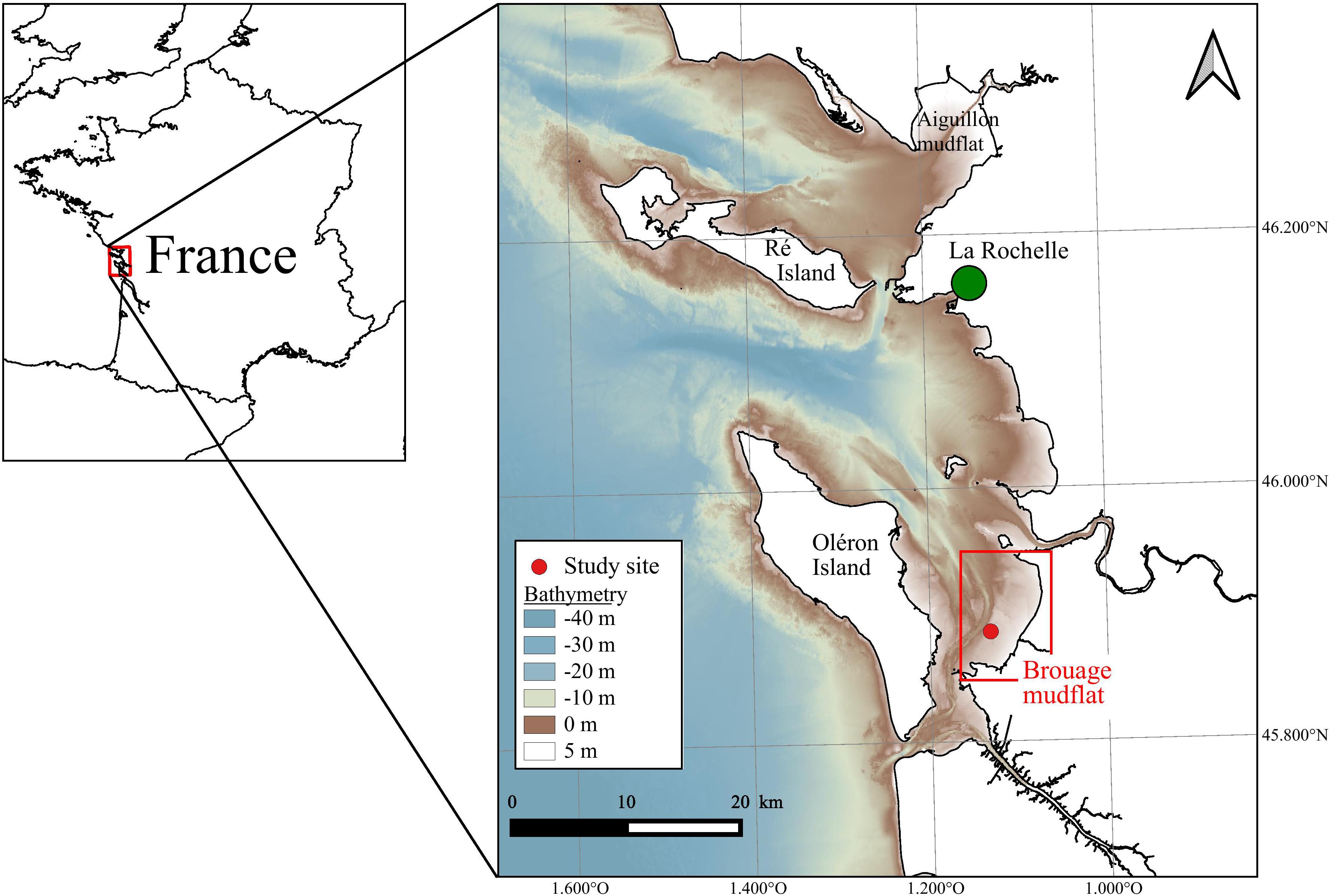
Figure 1. The Pertuis Charentais, and the Brouage mudflat, France. The red point indicates the study site. Bathymetry is used in MARS-3D model (source: SHOM).
Periods of Investigation
The investigated periods for MPB primary production estimation by multispectral remote sensing and modeling were selected in accordance to the seasonal cycle of MPB biomass (Figure 2). This cycle was extracted from a time series from 2000 to 2015, obtained by the processing of 582 low-tide images from the Moderate Resolution Imaging Spectroradiometer (MODIS) onboard the Terra satellite. MODIS Terra data [namely the Surface Reflectance Daily L2G Global 250 m SIN Grid product (MOD09GQ)] were used because the morning pass [10 to 11 h Universal Time (UT)] was better suited than the MODIS Aqua satellite afternoon pass to observe the emerged mudflat during spring low tides at our study site. The MOD09GQ product provides surface reflectance data in a red band (Rred, from 620 to 670 nm) and a near-infrared (NIR) band (RNIR, from 841 to 876 nm) at a spatial resolution of 250 m and with a revisit time of 1 to 2 days. This medium spatial resolution has been previously demonstrated to be valid for the study of MPB seasonal dynamics in large intertidal areas (van der Wal et al., 2010). For the present study, 582 MODIS low-tide images were initially downloaded, from which 343 cloud-free scenes were eventually selected. An NDVI (Eq. 1) was computed as a proxy of MPB biomass. The NDVI quantifies the changes in the reflectance’s spectral shape due to Chl a absorption in the red band and to the absence of absorption by pigments in the NIR plateau (Méléder et al., 2003b; Brito et al., 2013; Benyoucef et al., 2014; Echappé et al., 2018). The NDVI is a widely used vegetation index, relatively robust to the variability in sediment backgrounds (Barillé et al., 2011) and mainly driven by changes in algal biomass (i.e., the higher vegetation biomass, the higher the NDVI). Several methods have been developed to discriminate the MPB from other Chl-bearing intertidal vegetation (e.g., seagrass and macroalgae), from simple reflectance thresholds (Méléder et al., 2003b) to more complex clustering methods (Hossain et al., 2015). As previous field studies did not report significant areas colonized by macrophytes in the MPB-dominated Brouage mudflat (Lebreton, personal communication), the NDVI-derived biomass was non-ambiguously assigned here to MPB biofilms.
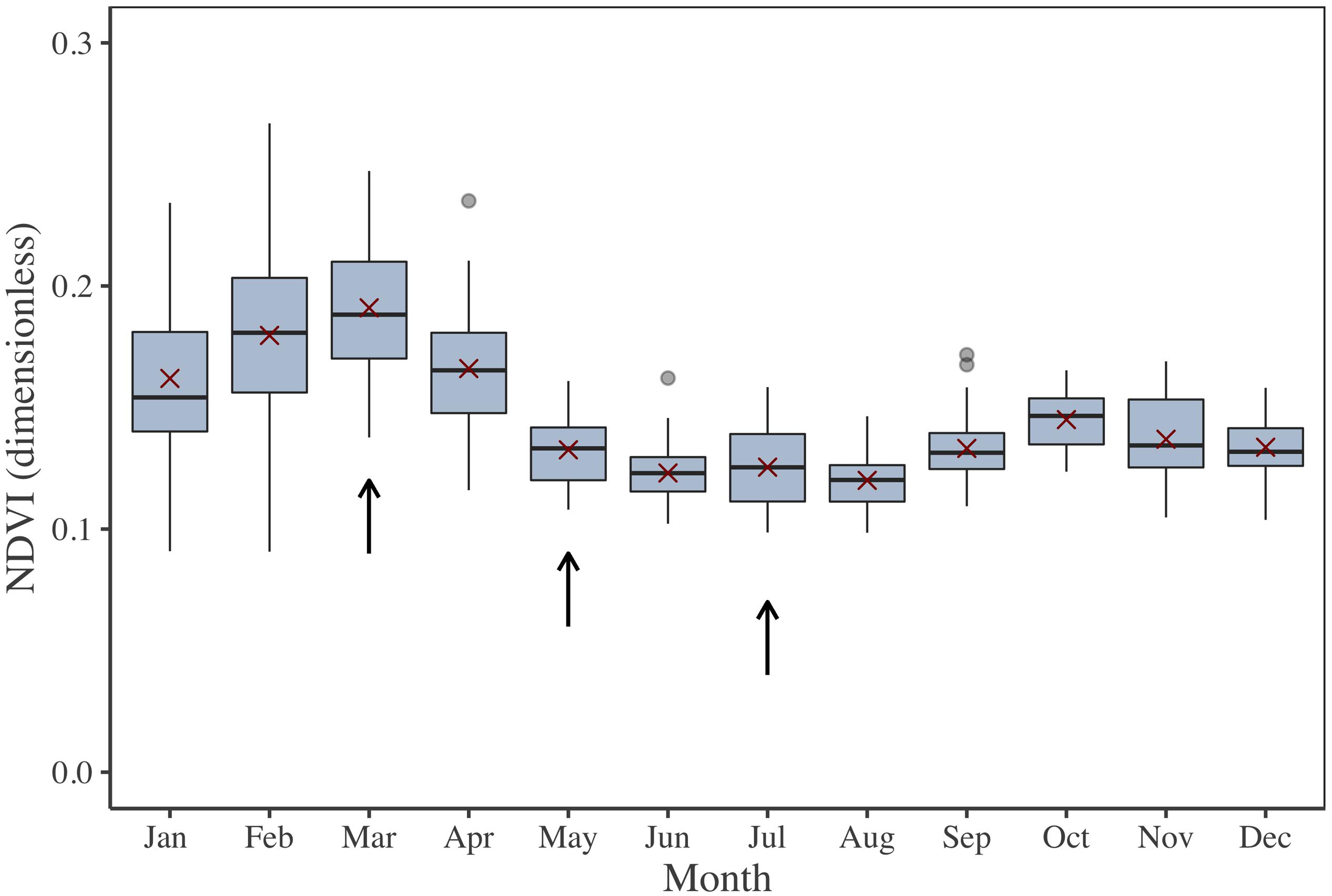
Figure 2. NDVI 2000–2015 time series illustrating the MPB biomass seasonal cycle for the Brouage mudflat. NDVI was retrieved from Terra MODIS reflectance. Box plots were calculated for each month. The red crosses are the monthly average. Arrows show the three period of investigation (March, May, and July).
From this NDVI time series, three periods were selected for field campaigns and for laboratory P–E curve calibration (Figure 2): March, when MPB biomass reaches its highest level; July, corresponding to the lowest level; and May, corresponding to an intermediary level. For the three periods, the weather was also expected to be contrasted: low temperature and light intensity in March, higher temperature and light intensity in July, and intermediate temperature and light in May. Field campaigns occurred the 5th and 6th of May, 2015; the 2nd and 3rd of July, 2015; and the 5th of March, 2018. They included in situ measurements and sediment sampling for further laboratory experiments.
Gross Primary Production (GPP) Measurements
Field Campaigns
The sampling station was located at the “Merignac” site, in the Brouage mudflat (Figure 1, red dot 45°53′11.20″N; 1°7′538″W). CO2 fluxes were measured at the air/sediment interface (enclosed sediment area of 165 cm2 down to 5-cm depth) using the closed-chamber method described in Migné et al. (2002). Air CO2 concentration (ppm) changes were monitored in the benthic chamber (0.8 L) continuously over an incubation period of 20 to 30 min, using an infrared gas analyzer (IRGA Li-840A, LI-COR, Lincoln, NE, United States) connected to a datalogger (Li-1400, LI-COR) with a 30-s frequency. CO2 flux was calculated as the slope of the linear regression of CO2 concentration (μmol mol–1) against time (min) and expressed in mg C m–2 h–1.
Transparent chambers were used to estimate the net benthic community production [NCP; balance between the community GPP and the community respiration (CR)]. Dark chambers were used to estimate the CR. Light and dark incubations were performed successively. Due to the tidal cycle duration, a maximum of four incubations were done per day (two transparents and two darks). The GPP expressed in mg C m–2 h–1 was computed following Migné et al. (2002) (Eq. 2):
The biomass-specific productivity (Pb) was then computed from GPP. Here, the NDVI was used as a proxy of MPB biomass, and Pb was directly expressed in C m–2 h–1 ndvi–1 (Eq. 3):
The NDVI was computed from MPB reflectance spectra acquired using a JAZ (Ocean Optics, Largo, FL, United States) spectroradiometer (200–1100 nm; sampling: 0.3 nm; spectral resolution: 0.3–10 nm FWHM) pointed at an area of the MPB biofilm close to the benthic chambers. Because the spectral resolution of this detector was higher than a satellite multispectral detector, NDVI calculation was adapted (Eq. 1): the red reflectance, Rred, was considered as the averaged value of data at 675 nm ± 3 nm and the NIR reflectance, RNIR, as the average at 750 nm ± 3 nm (Méléder et al., 2003a, 2010). NDVI was measured during the same period of each light incubations (equal to NCP estimation), and a time-averaged NDVI was used to standardize GPP in Eq. 3.
Synchronously, the incident photosynthetically active radiation (PAR, from 400 to 700 nm, in μmol photons m–2 s–1) and mud surface temperature (MST, in °C) were continuously (every 30 s) measured (LS-C sensor plugged to a ULM-500 data-logger, Walz, Effeltrich, Germany) at the sediment surface, near to the chambers and to the area of reflectance acquisition and measurement of MPB Chl a biomass content. The latter was measured in the first 250 μm of sediment continuously sampled (every 5–10 min) by the “crème brulée” technique (Laviale et al., 2015). This technique, derived from the contact-core technique (Ford and Honeywill, 2002), consists of freezing by contact the top surface of sediment (here 250 μm) with a metal surface (1.5 cm2) previously immersed in liquid nitrogen. The obtained sediment disks were stored in liquid nitrogen during field campaign and were kept at −80°C in the laboratory until pigment analysis. After freeze-drying of the sediment disks, pigments were extracted in a cold mixture (4°C) of 90% methanol/0.2 M ammonium acetate (90/10 vol/vol) and 10% ethyl acetate. Injection, HPLC device (Hitachi Lachrom Elite, Tokyo, Japan), pigment identification, and quantification were detailed before (Roy et al., 2011; Barnett et al., 2015). The Chl a amount in sediment was standardized to the sampled surface (1.5 cm2) in order to be expressed in mg Chl a m–2.
In an aim to assess MPB photophysiological status at tide time scale and check if changes occurred during incubation time, several photophysiological parameters (Fv’/Fm’, rETR, α, and Ek) were measured continuously (every 5 to 10 min) using a Water-PAM fluorimeter (Fiber version, Walz, Effeltrich, Germany). For details, see Supplementary Appendix A. All in situ data (GPP, PAR, MST, biomass, and photophysiological parameters) were used as ground-truthing for laboratory P–E curve calibration and the remotely sensed GPP validation.
Laboratory Experiment for Production–Irradiance Curve Calibration
During the three field campaigns, the upper layer (approx. the top first centimeter) of sediment was collected and brought back to the laboratory. The mud was cleaned of fauna by sieving through a 500-μm mesh. The sediment was homogenized by thoroughly mixing and was spread as plane layer in plastic trays of 4-cm depth (Serôdio et al., 2012). A water layer was added for the night and sediment was left undisturbed overnight. The next morning, the water layer was manually removed by a syringe 3 h before the lowest water level timing expected in situ (i.e., at sampling site) and trays were kept in darkness at 22 ± 1°C. Experimentation started 1 h later, when the MPB biofilm started to darken in color at the sediment surface. It consisted of lighting up the trays one by one with an LED panel (LED Light SL 3500-E, Photo System Instrument, Tøeboò, Czechia) at a given PAR (=E), varied from 5 to 2,200 μmol photons m–2 s–1 for 30 min at 22 ± 1°C, exactly in the optimal temperature range for MPB production (according to Blanchard et al., 1997). During the lightening, NCP was estimated through transparent benthic chamber incubations, following the same method as the field measurements (Migné et al., 2002). At the beginning and end of each light incubation, NDVI, sediment Chl a content, and photophysiological parameters using PAM-fluorimetry were measured the same way as in situ (see above). After illumination, CR was measured during the 20- to 30-min dark benthic chamber incubations. The same process was repeated as long as MPB was present at the surface of sediment (i.e., with similar measured NDVI) and for 8 to 11 Es. For each E, GPP was calculated as the sum between NCP and CR as done in situ (Eq. 2, Migné et al., 2002). GPP was then standardized by NDVI in order to directly express Pb in mg C m–2 h–1 ndvi–1 (Eq. 3), so that the GPP algorithm could be consistently applied to satellite-derived NDVI maps (see section “Coupling Remote Sensing Data and Modeling: the GPP-Algorithm”).
For the three campaigns (March, May, and July), a season-dependent Pb was obtained. For each season, several P–E models widely used in the literature [namely Platt et al. (1980), Eilers and Peeters (1988), Steele (1962), Platt and Jassby (1976), and the modified version of Platt and Jassby (1976)] were fitted to the P–E curves to select the best model to be integrated into the GPP-algorithm. The selection of the most appropriate model was done using the determination coefficient (r2) and residual standard deviation (RSD) calculated using the in R-software. For details, see Supplementary Appendix B.
Data Analysis for Field Campaign and Laboratory Experiments
All data are available for download: 10.5281/zenodo0.3862068. Changes in MPB biomass (NDVI and Chl a content), photophysiological parameters measured by PAM-fluorimetry (Fv’/Fm’, α, rETRm and Ek) and GPP and Pb were detected at a tidal time scale (i.e., during incubation) and at a monthly scale (March, May, and July). Knowing the potential high variability of environmental conditions (i.e., PAR, MST, and light dose calculated from PAR and emersion time), the objective was to check if biomass and photophysiological status changed drastically or not during the light incubation estimating GPP as well in situ and at the laboratory. In this aim, Spearman or Pearson correlations, and ANOVA or Kruskal–Wallis (KW) test were performed on all data using R software, after a Shapiro test, to test data normality. For details, see the Supplementary Appendix A.
Coupling Remote Sensing Data and Modeling: the GPP-Algorithm
The successive steps in the remotely sensed GPP procedure are described below and synthesized in Figure 3.
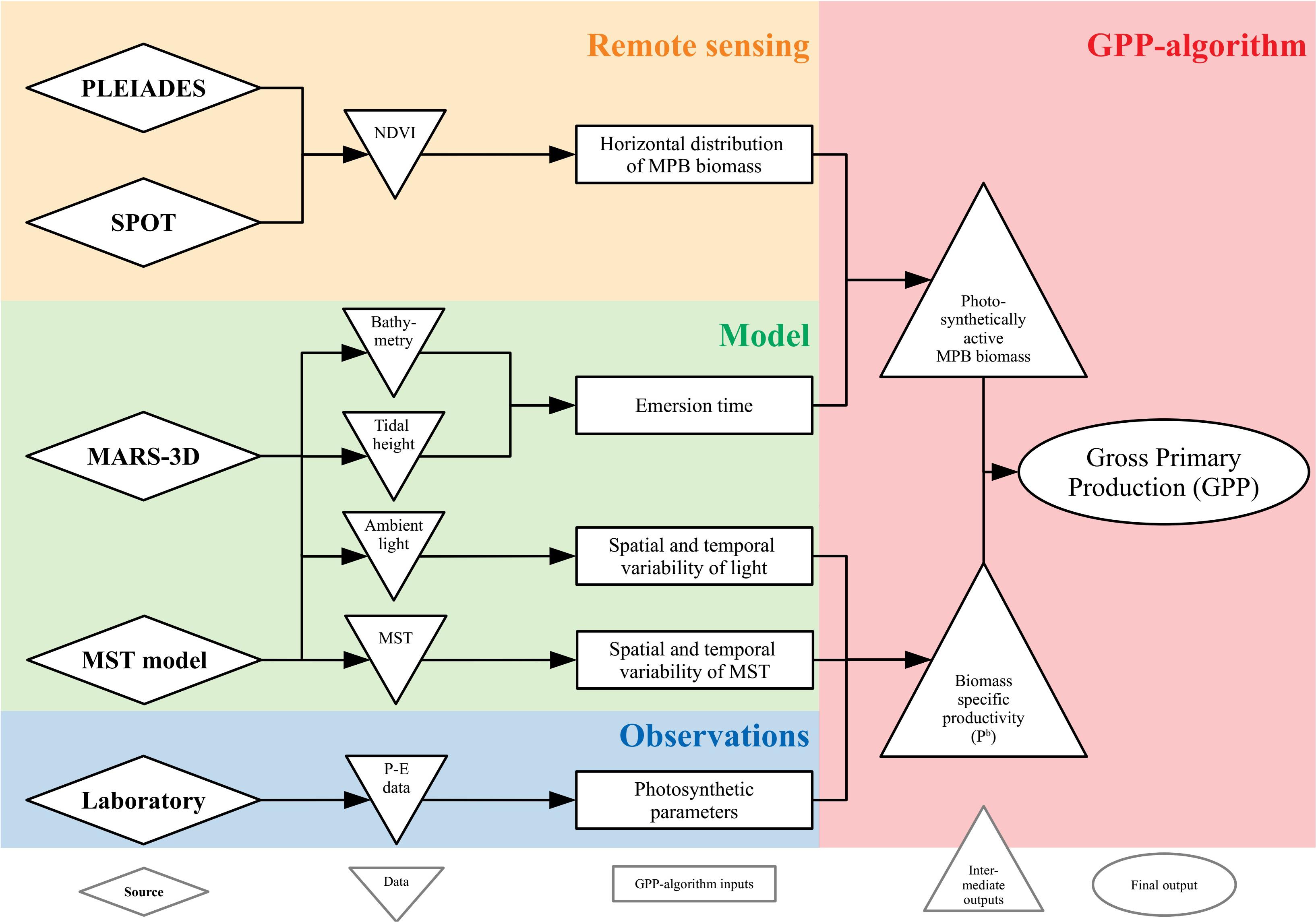
Figure 3. Conceptual scheme of the MPB GPP-algorithm.
Remote Sensing Data
High-resolution satellite remote sensing was used to upscale the GPP algorithm to the whole mudflat, using the season-dependent, NDVI-specific Pb parameter. Multispectral images were selected from the SPOT, Landsat, and Pléiades archives following three acquisition criteria: (1) acquisition day as close as possible to the field campaign day, (2) acquisition time as close as possible to low tide timing (i.e., the lowest water height, when mudflat was the most exposed), and (3) cloud-free observation (cloud cover < 10%) with an almost zenithal sun. These criteria allowed us to select three images from the SPOT6 and Pléiades archive (one per field campaign, Table 1). The top-of-atmosphere data were converted into surface reflectance using the fast line of sight atmospheric analysis of spectral hypercubes (FLAASH, Matthew et al., 2000) atmospheric correction using the ENVI software. For a consistent analysis of the SPOT and Pléiades images, the same FLAASH parameters were applied to each image: United States atmospheric model with a visibility of 40 km, and a maritime aerosol model. The spectral images were registered in the WGS 84 UTM 30N coordinate system. Finally, the NDVI was calculated from the surface reflectance following Eq. (1) to map MPB biomass (Méléder et al., 2003b). As the SPOT6 and Pléiades data have similar spectral characteristics, the NDVI was not recalibrated between the two sensors (Echappé et al., 2018). The satellite-derived NDVI maps were used as inputs for the GPP-algorithm, in complement to other data (Figure 3).
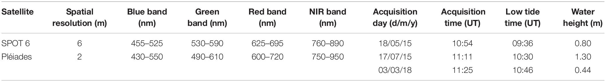
Table 1. Satellite image characteristics used to map the horizontal distribution of the MPB biomass, expressed in NDVI.
Tidal Height and PAR Modeling
The tidal height and PAR were simulated over the Brouage mudflat by the 3D hydrodynamical MARS-3D (Figure 3). The bathymetry was extracted from the model numerical grid. The Navier–Stokes primitive equations were solved under assumptions of Boussinesq approximation, hydrostatic equilibrium, and incompressibility (Blumberg and Mellor, 1987; Lazure and Dumas, 2008). The numerical domain of the Pertuis Charentais Sea consisted of 100- × 100-m grid cells discretized over 20 sigma-levels. For details, see Lazure and Dumas (2008). The meteorological forces (i.e., 10 m wind speed, 2 m air temperature and relative humidity, atmospheric pressure at sea level, nebulosity, and solar fluxes) used to constrain MARS-3D were extracted from the Meteo France AROME model1. The tidal model CST FRANCE, developed by the SHOM (Simon and Gonella, 2007), forced MARS-3D at the domain boundaries. The tidal model solved the amplitude and phase of 115 harmonic constituents. Initial and boundary conditions of seawater temperature, salinity, current velocity, and sea surface height were extracted from the MANGAE 2500 Ifremer model of 2.5-km lateral resolution (Lazure et al., 2009). Simulated tidal height associated to bathymetry allowed to estimate the beginning, the end and thus the duration of emersion period of each grid cells. During emersion period, PAR intensity varied every 10 min at 100- × 100-m spatial resolution, but values were interpolated on the horizontal grid of satellite data (2 or 6 m, see Table 1) and used as inputs in the GPP-algorithm (Figure 3).
Mud Surface Temperature Modeling
The simulated mud surface temperature (MST) was obtained from the coupling of the MST model of Savelli et al. (2018) with MARS-3D. The simulated heat fluxes in a 1-cm-deep sediment layer were solved by thermodynamic equations detailed in Savelli et al. (2018). The horizontal fluxes of heat were neglected. During exposure periods, the simulated MST resulted from heat exchanges between the sun, the atmosphere, and the sediment surface; from the conduction between mud and air; and from evaporation. The simulated MST of immersed mud was set to the temperature of the overlying seawater simulated by MARS-3D since MST was not used in this study. The MST differential equation was solved by the MARS-3D numerical scheme. For more details, see Savelli et al. (2018). During emersion period, MST varied at the same time resolution than PAR intensity (10 min and 100 × 100 m). But, as PAR, the MST values were interpolated on the horizontal grid of satellite data (2 or 6 m, see Table 1) and was used as input in the GPP algorithm (Figure 3).
GPP Algorithm
Finally, the GPP algorithm (Figure 3) coupled NDVI maps from SPOT and Pléiades scenes with forces by hydrodynamical MARS-3D. Whereas the NDVI estimates the horizontal distribution of MPB biomass, the MARS-3D model simulates the emersion time over the whole mudflat using the bathymetry and the tidal height. Coupled with the MPB biomass, the emersion time determined the photosynthetically active biomass at the mud surface. The MPB biomass detected by satellite was assumed to correspond to the fully established biofilm during the daytime low tide (total photosynthetically active biomass). The migration behavior of MPB was introduced in the model through a progressive establishment of the total photosynthetically active biomass at the sediment surface, known to take place during 20 min at Brouage mudflat (Herlory et al., 2004). The MPB started to migrate at the sediment surface just after water removal to reach 50% of the total amount of the photosynthetically active biomass (=NDVI/2) after 10 min of emersion of respective grid cells. After 20 min, the MPB biofilm at the sediment surface was fully formed. 20 min before the immersion, downward migration started and only the half of the total photosynthetically active biomass was still at the surface 10 min before immersion. No biomass was at the surface when water overlaid the sediment. PAR and MST simulated by MARS-3D were used to constrain the algorithm: the selected P–E model and its respective parameters values fitted on the laboratory measurements were used to compute the Pb according to the simulated light conditions. The effect of MST was simulated using the Blanchard et al. (1996) model to compute the Pb variations according to the simulated temperature. Finally, combined with the horizontal distribution of the MPB biomass of the NDVI maps, the Pb (mg C m–2 h–1 ndvi–1) was further used to map the remotely sensed GPP (mg C m–2 h–1). The time resolution was 10 min (following PAR and MST variations), whereas the spatial resolution was the one of the SPOT or Pléiades image (2 or 6 m, see Table 1).
The current configuration of the GPP-algorithm was consistent only for intertidal mudflats composed by very fine cohesive grains over the Brouage mudflat (Poirier et al., 2010). Consequently, no-muddy areas were excluded of the GPP-algorithm and MST model used was developed and validated for the mud only (Savelli et al., 2018). Therefore, laboratory and in situ measurements were conducted only on muddy sediment. The GPP maps thus corresponded to MPB assemblages known to be dominated by epipelic diatoms at the study site (Haubois et al., 2005; Du et al., 2017).
GPP Maps Validation
The validation of the GPP model was performed in three steps for each seasonal experiment, using the field data acquired at the study site (see section “Gross Primary Production (GPP) measurements”). First, the simulated MST and PAR were compared to in situ measurements using a Mann Whitney (MW) test to assess the accuracy of the physical model. Second, the satellite derived NDVI was validated against field measurements. The GPP was then computed from satellite-derived NDVI maps coupled with the modeled PAR and MST data. The remotely sensed GPP maps were averaged hourly (mg C m–2 h–1) over the emersion period, as well as daily-integrated period (mg C m–2 d–1). Finally, the hourly remotely sensed GPP data was compared to in situ GPP measurement using a MW test.
To ensure that the delay between measurements for P–E calibration and image acquisition (2, 13, and 14 days in March, May, and July, respectively) was not an issue, simulated PAR were averaged during daytime emersion periods 2 weeks before each sampling/measurement session and image acquisition to be compared (MW tests). The main limitation was a change in physiology and metabolic acclimation status of MPB cells due to a change in light and temperature conditions during this delay, preventing the use of P–E photophysiological parameters retrieved from laboratory experiments to calibrate images acquired several days later.
Results
Microphytobenthos GPP Variation Between Months
Field Campaigns
During field campaigns, PAR intensity and MST were significantly different between months (Figures 4a,b; KW test, p ≤ 0.001). Minimum values were mainly measured in March for PAR and MST with 624 ± 10 μmol photons m–2 s–1 (mean ± SE) and 15.7 ± 0.1°C, respectively, whereas maximum values were reached in May for PAR (1,509 ± 27 μmol photons m–2 s–1) and July for MST (30.7 ± 0.2°C) (Figures 4a,b). According to its seasonal cycle (Figure 2), MPB biomass was higher in March than in May and July (KW test, p≤0.001) with averaged NDVI values and Chl a sediment content of 0.61 ± 0.01 and 95.2 ± 3.1 mg m–2, respectively (Figures 4c,d). The GPP did not vary significantly among campaigns, although the minimum value was measured in March, and the highest was measured in July (Figure 4e). When GPP was standardized by NDVI to be expressed into biomass-specific productivity (Pb), this difference was more visible (Figure 4f) even if it was not significant (KW test, p = 0.1). Regarding photophysiological parameters measured by PAM-fluorimetry (Fv’/Fm’, α, rETRm, and Ek), see Supplementary Appendix A. At the tidal scale, biomass (NDVI and Chl a content), but also PAM photophysiological parameters (Fv’/Fm’, α, rETRm, and Ek) changed with PAR, light dose, and MST, illustrating the rapid responses of MPB (behavioral migration and/or physiology) to environmental conditions.
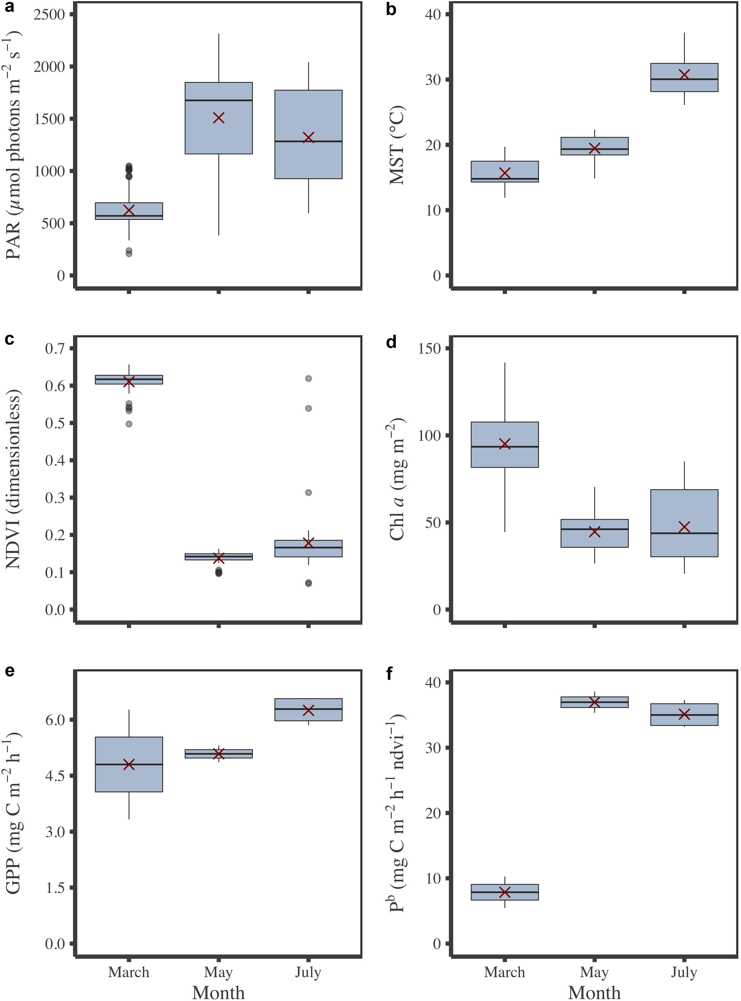
Figure 4. Monthly variations of environmental and MPB parameters measured in situ. PAR (a), MST (b), biomass in NDVI (c) and Chl a content (d), GPP (e) and Pb (f). Red crosses correspond the mean values for the corresponding period.
Laboratory Measurements for P–E Curve Calibration
During laboratory experiments, whereas temperature and PAR were controlled, the MPB biomass, expressed in NDVI or Chl a sediment content, changed with the sampling campaign date; as for in situ, it was the highest in March, with an averaged value of 0.57 ± 0.01 for NDVI and 97.7 ± 5.5 mg Chl a m–2 (three-way ANOVA, p ≤ 0.001; Figure 5 and Supplementary Table A3). The biomass at the sediment surface of the plastic trays globally did not change between PAR tested and during incubation time for a given month (see Supplementary Table A3 for details). Consequently, GPP measured from benthic chamber incubations for each sediment tray were considered to correspond to a same MPB biomass. Biomass specific productivity, Pb was then obtained by dividing GPP by the averaged NDVI value over the sediment trays for each month: 0.57 ± 0.01 in March, 0.08 ± 0.01 in May, and 0.20 ± 0.01 in July (Supplementary Figure A3a). The shape of the relationship between Pb and the irradiance provided by artificial lighting (i.e., P–E curves) varied with seasons (Figure 5), as well the fitted photophysiological parameters from the five P–E models tested (Supplementary Table B1). The high r2 and low RSD values demonstrated that all P-E models fitted well with the laboratory measurements (Supplementary Table B2). Because it exhibited the best fit to P–E laboratory measurements, the Eilers and Peeters (1988) model was selected to estimate and map remotely-sensed GPP using the GPP-algorithm.
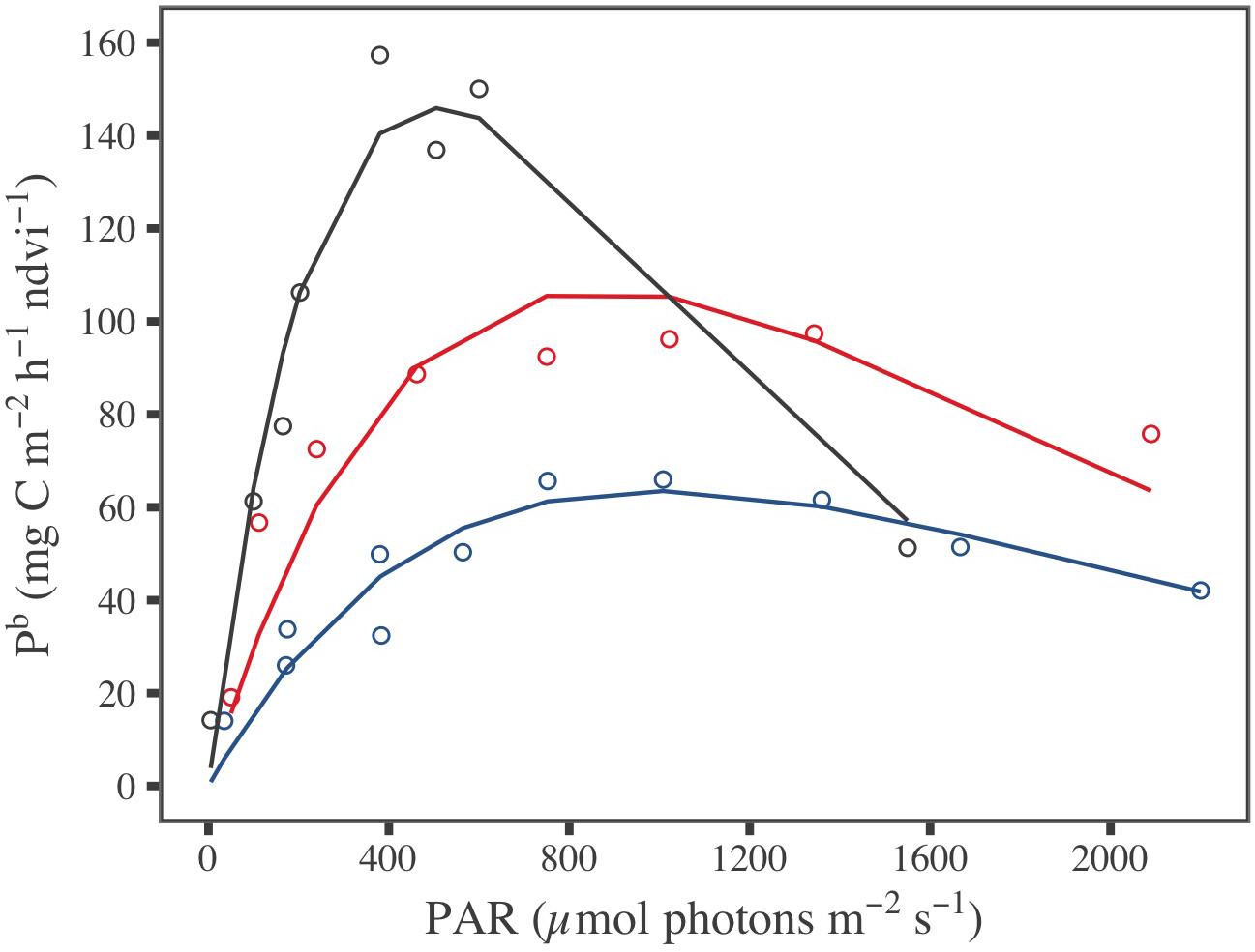
Figure 5. Measured (dot) and predicted (line) biomass specific productivity (Pb) standardized by NDVI, fitted with the Eilers and Peeters (1988) P–E model for the three periods of investigation: March (blue), May (gray), and July (red).
Mapping Microphytobenthos GPP From NDVI Maps
Overall, SPOT and Pléiades provided consistent spatial distribution of MPB biomass, with a higher NDVI in the middle and lower areas of the mudflat than in the upper shore, especially in March and May (Figure 6). The Pléiades-derived NDVI varied from 0 to 0.4, with an averaged value of 0.2 ± 0.09 in March and of 0.14 ± 0.05 in July (Figures 6a,c), whereas the SPOT6-derived NDVI varied from 0 to 0.3, with an averaged value of 0.14 ± 0.05 in May (Figure 6b). Besides the seasonal variability, the difference in the sensors’ spatial resolution could also partly explain the differences between SPOT6 and Pléiades. Compared to Pléiades (2 m), the lower spatial resolution of SPOT6 (6 m) smoothed out the fine-scale distribution of MPB biofilms, thus resulting in lower NDVI averages.
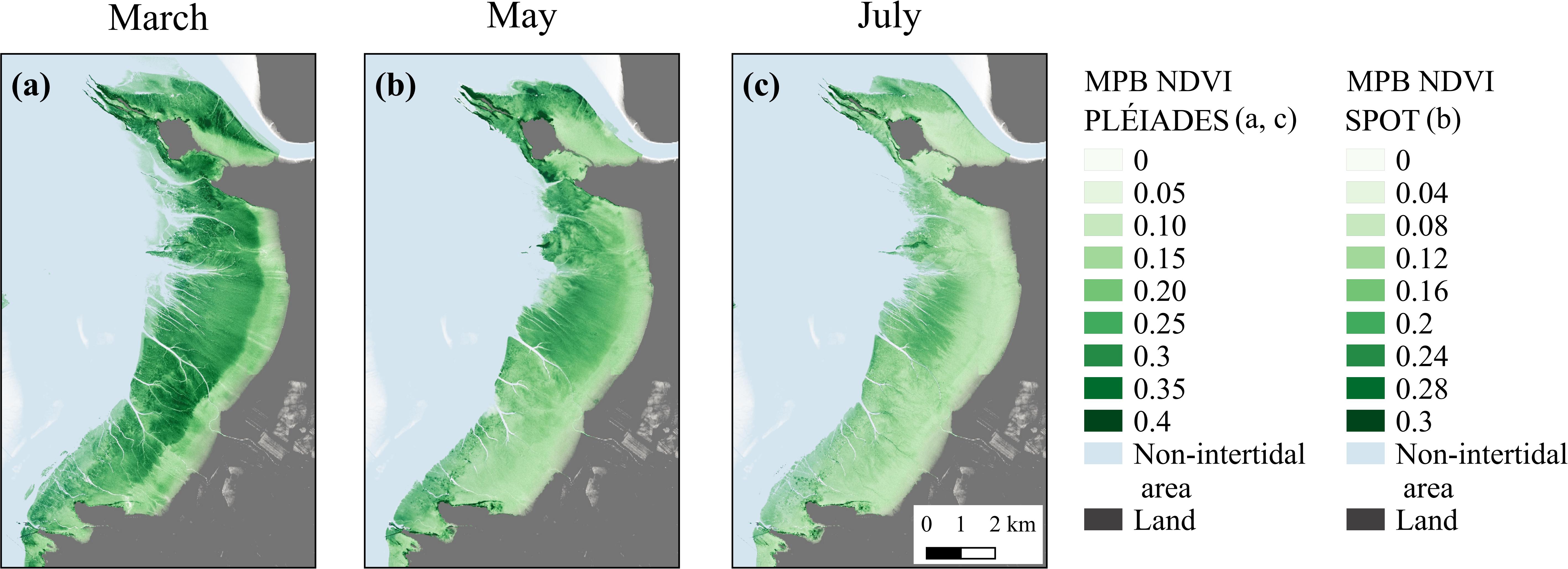
Figure 6. MPB-specific NDVI from Pléiades satellite, March 3, 2018 (a), and July 17, 2015 (c), and from SPOT6 satellite, May 6, 2015 (b).
Spatially resolved GPP rates were then modeled from the satellite-derived NDVI maps for each season (Figure 7). The short-scale temporal variability of the production factors was taken into account using the hourly PAR and MST MARS-3D simulations and the laboratory P–E curves (Figure 5 and Supplementary Table B1). For each date of satellite acquisition, remotely sensed GPP was averaged over the daytime emersion period (Figures 7a–c) and eventually integrated to yield daily GPP maps (Figures 7d–f). GPP was at its maximum in March and its minimum in July (Figures 7a,c). The most productive areas of the mudflat were the middle and lower shores, with values up to 14.4 mg C m–2 h–1 in March and 10.8 mg C m–2 h–1 in May (Figures 7a,b). The upper shore was less productive with an hourly GPP of ∼7.5 mg C m–2 h–1 in March and ∼6.0 mg C m–2 h–1 in May (Figures 7a,b). The hourly GPP exhibited no spatial pattern in July, and GPP was low over the entire mudflat (∼1.8 mg C m–2 h–1, Figure 7c). The mean daily-integrated GPP, reaching 50.2 ± 30.1 mg C m–2 d–1 in March, 40.9 ± 26.8 mg C m–2 d–1 in May, and 22.3 ± 20.5 mg C m–2 d–1 in July, allowed to integrate GPP over the mudflat, reaching, respectively, 2.06 (for an emerged surface of 41 km2), 1.42 (for 34.5 km2), and 0.80 tC d–1 (for 36 km2) in March, May, and July (Figures 7d–f).
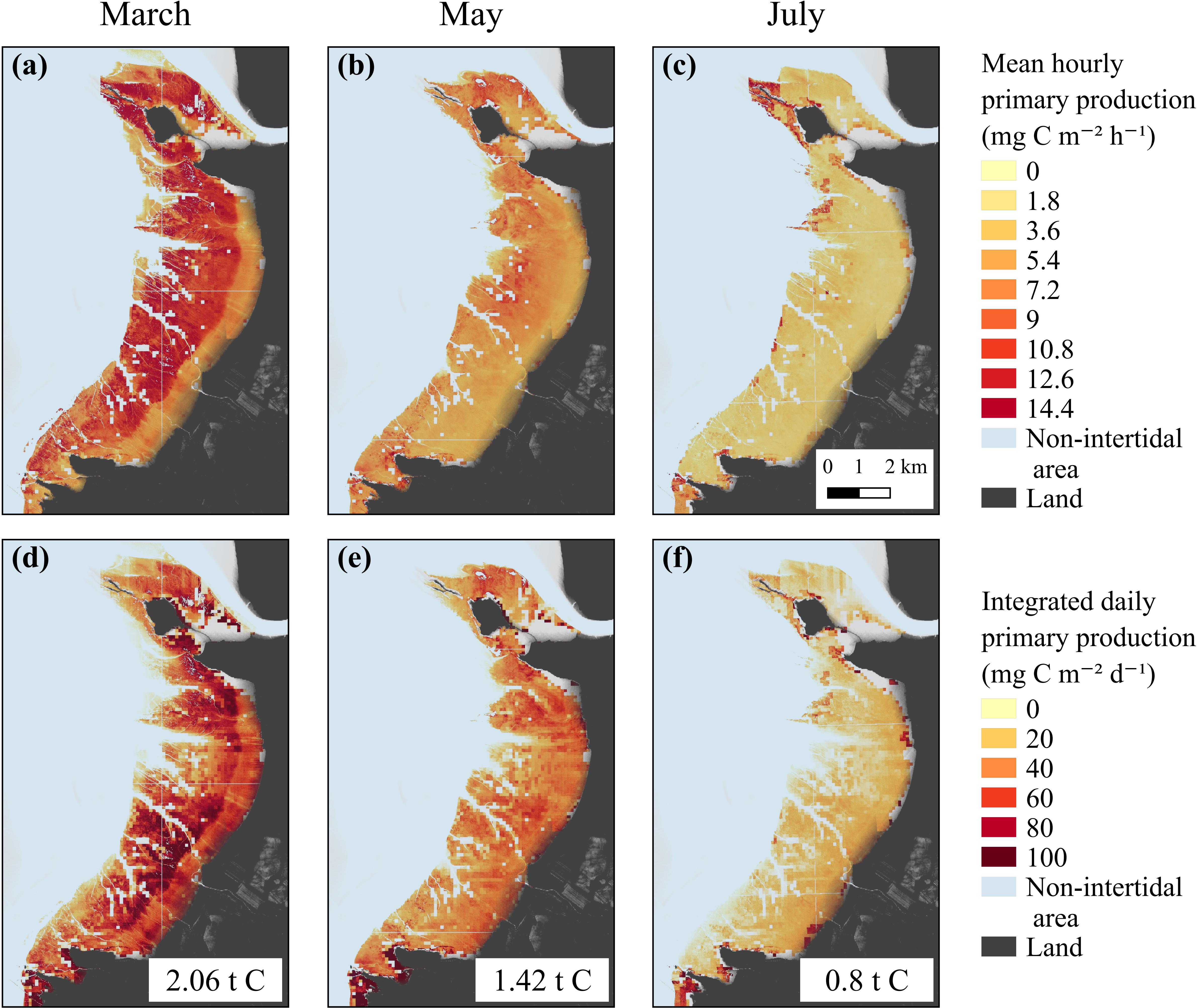
Figure 7. Hourly (mg C m–2 h–1) and daily (mg C m–2 d–1) averaged remotely-sensed GPP from the GPP-algorithm based on Eilers and Peeters (1988) P–E model in March (a,d), May (b,e), and July (c,f).
Validations
A Priori Physical Environment Validation
The MST and PAR conditions simulated by the MARS-3D model satisfactorily compared to the in situ conditions, even if there were some significant differences (Figures 8a,b). The delay between field campaigns and image acquisition was not an issue (Figures 8c,d): for the three periods, the averaged PAR and the MST 2 weeks before measurements and before images acquisition were not significantly different (Figures 8c,d). These observations mean that MPB cells were expected to be in a similar acclimation status during laboratory experiments and image acquisition. After these first validations, simulated MST and PAR, satellite images and calibrate P–E model were used in the GPP algorithm to predict and map GPP.
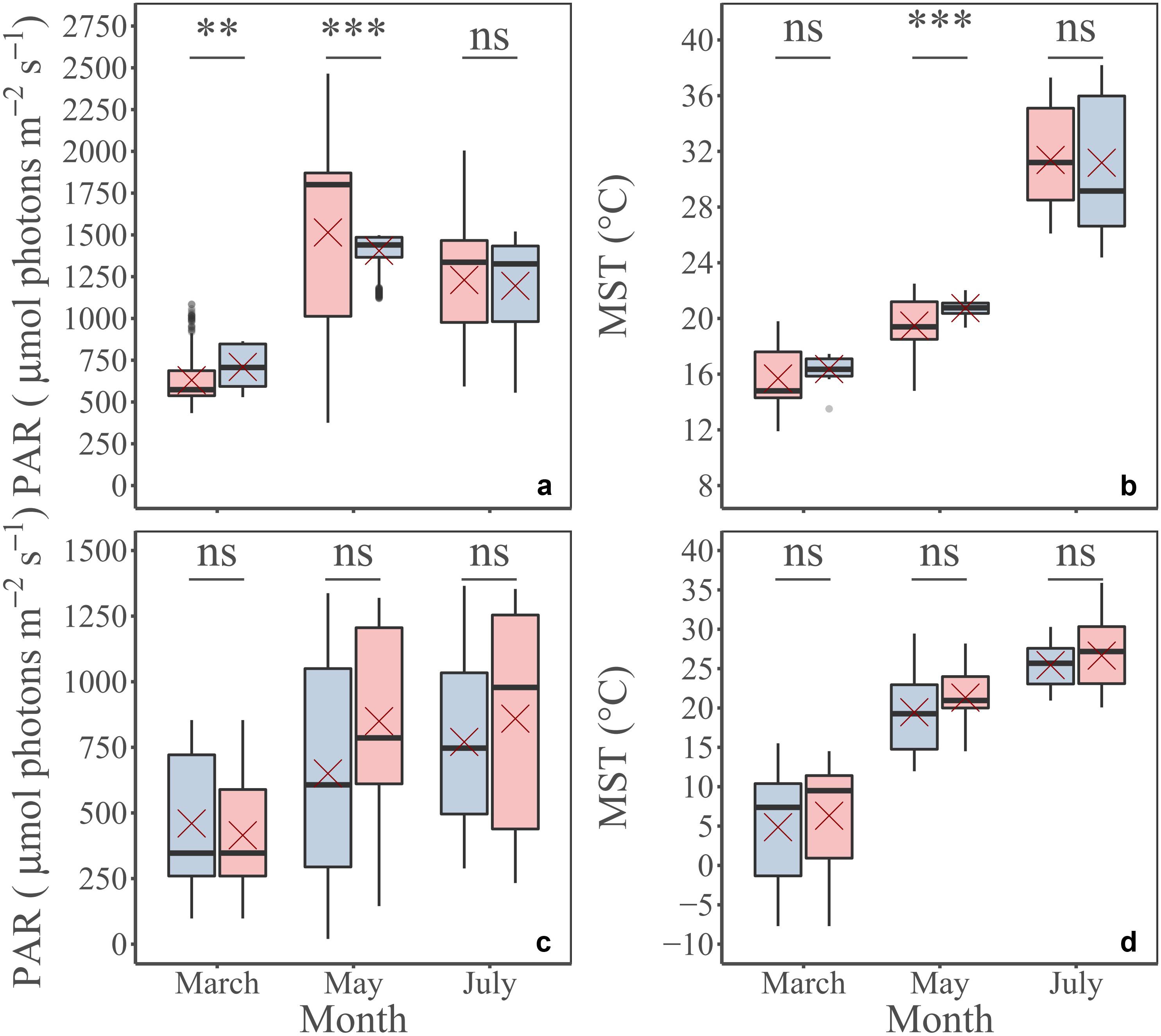
Figure 8. A priori physical environment validation. PAR (a) and MST (b) measured in situ (blue) and simulated by MARS-3D (pink) for the same period: March, May, and July; PAR (c) and MST (d) simulated by MARS-3D, averaged during daytime emersion periods 2 weeks before in situ measurements (blue) and satellite scenes acquisitions (pink). Red crosses correspond the mean value of PAR and MST for the corresponding period. Mann Whitney test; p-value: ns, p > 0.01; *p ≤ 0.01; **p ≤ 0.001; ***p ≤ 0.0001.
Measured Versus Estimated NDVI and GPP
The NDVI measured in situ was always higher than the remotely sensed NDVI at the study site (Figure 9a). In March, the NDVI measured in situ (0.61 ± 0.03) was almost 5-fold higher than the remotely sensed NDVI at the pixel corresponding to the study site (0.14). The NDVI measured in situ in May (0.14 ± 0.02) was 1.5-fold higher than the remotely sensed NDVI at the pixel of the study site (0.09). In July, the NDVI measured in situ (0.18 ± 0.09) was almost 1.8-fold higher than the remotely sensed NDVI at the pixel of the study site (0.1). Regarding the GPP, the measured value in situ varied from 4.8 ± 2.1 mg C m–2 h–1 in March to 6.3 ± 0.3 mg C m–2 h–1 in July (Figures 4e, 9b), whereas the GPP remotely-sensed at the respective grid cell averaged during daytime emersion varied from 2.2 ± 1.4 mg C m–2 h–1 in July to 7.8 ± 3.1 mg C m–2 h–1 in March (Figure 9b). However, there was not significant difference between in situ and remotely sensed GPP (MW tests, Figure 9b).
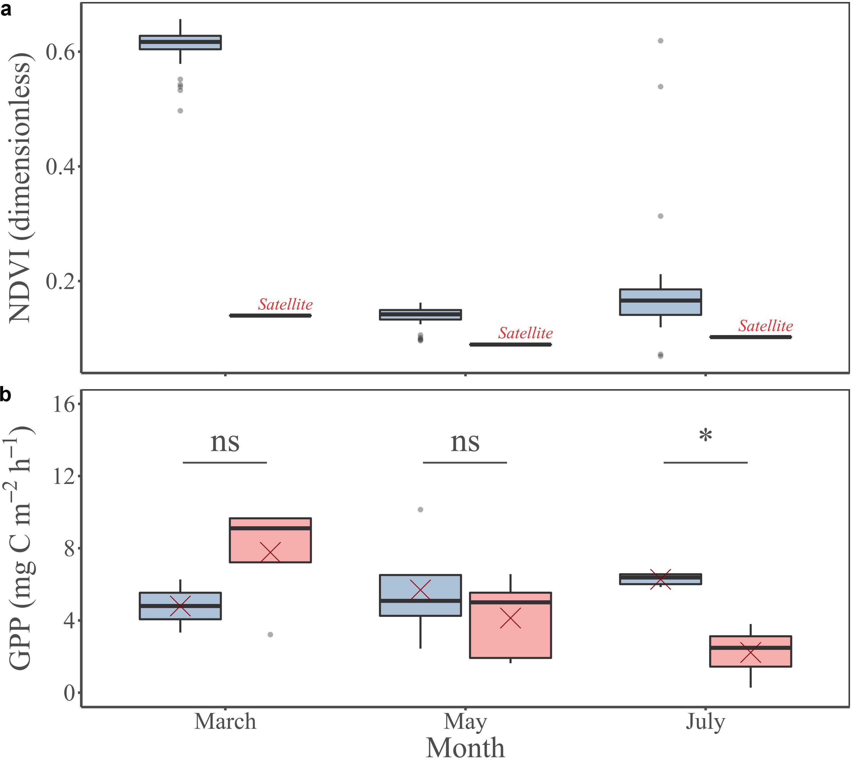
Figure 9. MPB-specific NDVI (a) and GPP (b) measured in situ (blue) and remotely sensed (pink) at the study site for the three investigated periods: March, May, and July. Red crosses correspond the mean values for the corresponding period. Mann Whitney test, p-value: ns, p > 0.01; *p ≤ 0.01; **p ≤ 0.001; ***p ≤ 0.0001.
Discussion
NDVI Versus Chl a GPP Standardization
In order to be able to upscale MPB biomass over an entire mudflat, NDVI has been used as a proxy of MPB abundance (e.g., Méléder et al., 2003b; van der Wal et al., 2010; Brito et al., 2013; Benyoucef et al., 2014; Echappé et al., 2018). Here, the NDVI 2000–2015 time series demonstrated a seasonal cycle characterized by a maximum of MPB biomass in winter–spring and a minimum in summer. This MPB seasonality observed in the Brouage mudflat is consistent with the seasonal pattern reported before for the same mudflat (Cariou-Le Gall and Blanchard, 1995; Savelli et al., 2018) and for other Northern European mudflats (van der Wal et al., 2010; Echappé et al., 2018).
Usually, on a local scale, GPP is standardized to the Chl a sediment content (e.g., Cahoon, 2006). Ideally, in order to convert our NDVI maps into GPP, a conversion of NDVI in Chl a sediment content should be performed. However, a direct relationship between NDVI and Chl a is a real issue for three main reasons. First, the relationship is known to be non-linear and to saturate for high values of Chl a (Méléder et al., 2003a; Serôdio et al., 2009; Barillé et al., 2011; Daggers et al., 2018). Second, there is an ongoing debate on the sediment depth to be sampled for Chl a content estimation in order to be in accordance with the sediment depth detected by sensors for NDVI calculation. Jesus et al. (2006) suggested the sampling of the first 150 μm, however, all depths tested along the first 2 mm were highly correlated, leading to similar NDVI for different Chl a contents (i.e., different depths). Moreover, the optical depth varies with the MPB biomass at the sediment surface, the sediment texture, the organic and water content, and the incident light wavelengths (Kühl et al., 1994; Jesus et al., 2006; Barillé et al., 2011; Kazemipour et al., 2011; Fisher et al., 2018). In the current study, the length of the path of the reflected light (i.e., the NDVI) is assumed to correspond to the photic zone, where the biomass is photosynthetically active, which rarely exceeds 500 μm for muddy sediments (Cartaxana et al., 2011). Third, the dilution of the reflectance signal from the sediment surface to the satellite sensor is variable. MPB-specific NDVI data obtained in this study from MODIS-Terra, SPOT6, and Pléiades satellites and measured in situ with a handheld field spectroradiometer reach, respectively, maximal values of 0.25, 0.30, and 0.40 for satellite and 0.60 in situ, meaning that maximum NDVI value decreases with spatial resolution. Even if such values are in the range of the MPB-specific NDVI derived from satellite data over temperate mudflats (Méléder et al., 2003b; van der Wal et al., 2010; Brito et al., 2013; Benyoucef et al., 2014; Echappé et al., 2018), their variability illustrates the different sensitivity between devices, but also the dilution of the reflectance signal for larger surfaces, mainly due to the patchiness distribution of the MPB biofilm (Saburova et al., 1995; Jesus et al., 2006; Spilmont et al., 2011). Méléder et al. (2010) and Launeau et al. (2018) demonstrated previously that MPB patchiness is responsible for a reflectance signal, due to the non-linear mixing of individual MPB patches and apparent mud. This generates one Chl a content corresponding to diverse NDVI values and conversely, one NDVI value could correspond to diverse Chl a content. This non-linear mixing increases the difficulty to use the Chl a sediment content measured at local scale (a few millimeters squared) to map NDVI over several meters squared or kilometers squared. In the present study, the direct calibration of the GPP-algorithm in NDVI allowed to decrease bias due to uncertainties of the NDVI versus Chl a relationship. Nevertheless, and in spite of this major improvement, some issues remain, such as the NDVI saturation for high MPB biomass leading to a potential non-linear GPP-NDVI relation, which will need further investigation.
GPP Algorithm Physical Setting
The MST and PAR conditions simulated by the MARS-3D model compared well to the conditions measured in the field. The model-versus-in situ data comparison suggested that the 3D model can resolve with confidence the physical environment experienced by MPB at the sediment surface. In regards to the frequency of the atmospheric AROME model (1 h), the simulated PAR conditions varied less than the in situ observations. The 3D model could not reproduce the observed synoptic variations of irradiance at the sub-hourly scale that can induce a substantial variability in the remotely sensed GPP over an emersion period. In addition, the horizontal resolution of the 3D model (100 × 100 m) may also translate into model–data discrepancies. In the GPP-algorithm, the bathymetric level and simulated water height originating from 100- × 100-m grid cells delay the emersion timing by ∼30 min. However, considering this delay, the comparison of in situ and simulated physical conditions and GPP were made on the corresponding low tides. Most importantly, the preservation of the horizontal resolution of satellite data in order to capture the MPB patchiness suggests that the GPP algorithm can resolve with confidence the overall dynamics of MPB GPP at the tidal scale.
Ability of the GPP Algorithm to Map the Current Productive State of the Mudflat
Our study is not the first to assess MPB primary production coupling remotely sensing and physical–biological modeling. Daggers et al. (2018) proposed a first approach using (i) remotely sensed information on MPB biomass and on sediment mud content, (ii) surface irradiance and ambient temperature, (iii) directly measured photophysiological parameters by PAM fluorimetry, and (iv) a tidal model. The current GPP algorithm improves the (Daggers et al., 2018) approach by (i) the use of NDVI rather than the conversion of NDVI into Chl a, which introduces uncertainties (see section “Discussion” above); (ii) the use of MST rather than ambient temperature, which was identified as a weakness of their model; and (iii) photophysiological parameters derived directly from benthic chamber CO2 exchange measurements on natural MPB communities in sediment under controlled conditions, rather than an averaged electron requirement (EE) rate derived from PAM fluorimetry. The EE used by Daggers et al. (2018) corresponds to the ETR efficiency for C fixation to translate ETR (μmol electrons m–2 s–1) into C (mg C m–2 h–1). However, it is known to vary with season, species, and site (Barranguet and Kromkamp, 2000), and the relationship between ETR and C-fixation can be non-linear, especially at irradiances exceeding Ek. The difficulty to use photophysiological parameters derived from PAM fluorimetry to predict C fixation was confirmed by the current study. PAM photophysiological parameters could vary rapidly even during the time of benthic chamber incubation (30-min duration) rendering the use of an averaged EE rate weakly representative of a given season, a given day and even a given emersion. To overcome this issue, we suggest to directly calibrate the P–E model with C-fixation standardized to NDVI values.
Additionally, the environmental conditions 2 weeks before measurements for the GPP algorithm calibration and 2 weeks before the acquisition of satellite images used to apply GPP algorithm were checked in the aim to support the representativeness of the photophysiological parameters. The conditions were similar, assuming the same photosynthetic capabilities of MPB during experiments for the calibration and during image acquisition. Otherwise, it would have been hazardous to apply the GPP algorithm on MPB that would have been differently acclimated between lab experiments and satellite image acquisitions.
The GPP algorithm uses a vertical migration scheme of MPB biomass within the upper layer of sediment, which is represented through the modulation of the total photosynthetically active biomass detected from the remotely sensed NDVI. Such a migration scheme in the GPP algorithm was set according to the observation of the progressive superficial sediment covering by MPB during emersion at our study site (Herlory et al., 2004). However, the migration speed can be faster [a few minutes; see Méléder et al. (2003b)] or slower [one hour; see Paterson et al. (1998)], and it is mainly controlled by the tidal cycle and the light climate and spectral quality (Pinckney and Zingmark, 1991; Spilmont et al., 2007; Coelho et al., 2011; Barnett et al., 2020; Prins et al., 2020), but also by temperature (Cohn et al., 2003), nutrient availability in the sub-surface of sediment (Kingston, 2002), and desiccation (Coelho et al., 2009). Currently, the GPP-algorithm does not include the short-term variations of MPB photosynthetically active biomass at the sediment surface (i.e., “micro-migrations”), as it has been also observed some days/timings during our field campaigns. As suggested previously by Daggers et al. (2018), further research on the mechanisms and triggers that determine the vertical phototaxis of diatom cells in sediment is required to better predict and model intertidal MPB migration patterns and therefore changes in MPB photosynthetically active biomass at the sediment surface.
When constrained by the PAR and MST conditions simulated by the MARS-3D model, the remotely sensed GPP predicted by the GPP-algorithm reached rates up to 14 mg C m–2 h–1 or 100 mg C m–2 d–1, similar to rates reported for other European mudflats (Barranguet et al., 1998; Underwood and Kromkamp, 1999; Cahoon, 2006; Hubas et al., 2006; Daggers et al., 2018; Frankenbach et al., 2020). These values further supports the key role of MPB in supporting the high productivity of temperate intertidal bare mudflats (e.g., Cahoon, 1999; Underwood and Kromkamp, 1999; Barranguet and Kromkamp, 2000) and its paramount support to local socio-economics (Lebreton et al., 2019). This growing recognition also supports the necessity for the worldwide consideration of mudflats as key ecosystems in the marine global carbon budget (Ciais et al., 2014; Legge et al., 2020).
The predicted and measured GPP reasonably compared. Both GPP show low seasonal variability, whereas the MPB biomass displays a pronounced seasonal cycle. This leads to lower Pb values during the period with the highest MPB biomass (i.e., March). It has been shown before that high MPB biomass does not always generate high production (Barranguet et al., 1998). During winter, the MPB biomass standing stock increases due to lower grazing activity (Thompson et al., 2000). As a consequence, MPB photosynthetically active biomass is mainly concentrated in an extremely thin layer at the sediment surface. However, such high concentration induces strong competition for light and nutrients, limiting the biomass specific productivity (Pb) (Barranguet et al., 1998; Stal, 2010; Vieira et al., 2016). This competition, compensated by high biomass, suggests a bottom-up regulation of the GPP in winter (by light, temperature, and nutrients), whereas a top-down control (by grazing activity) occurs in spring and summer.
Conclusion and Perspectives: The Use of Hyperspectral Remote Sensing
The GPP algorithm developed in this study combines satellite remote sensing, laboratory measurements, and a 3D physical model. The algorithm is constrained by realistic simulated 2D fields of tidal heights, MST, and PAR. It is standardized by photophysiological parameters estimated from laboratory measurements on natural MPB communities in sediment and expressed in C fixation rates. In addition, the direct calibration of the algorithm in NDVI is a step forward to limiting outstanding bias due to NDVI to Chl a conversion. Moreover, the calibration of the GPP algorithm to NDVI allowed us to consistently apply the algorithm to satellite images. This study shows that:
• The NDVI data retrieved from the SPOT6 and Pléiades sensors were consistent with the seasonality of the MPB biomass previously reported for the study site, and their range was comparable to NDVI data from other European mudflats;
• The GPP-algorithm yields MPB GPP rates in the range of in situ GPP measurements, including the seasonal variability of GPP;
• The GPP algorithm was well-adapted to intertidal mudflats mostly composed by fine cohesive sediments dominated by motile epipelic diatoms, and it could be applied for similar habitats.
However, this study highlights several challenging issues that need to be tackled to better estimate MPB production on regional and global scales from in situ information:
• Photosynthetic ability changes over a range of time scales, from the emersion to the season via the tidal fortnight cycle. To overcome this issue, photophysiological parameters, and not only MPB biomass, have to be measured at the ecosystem level (i.e., entire mudflat scale). Currently, only hyperspectral remote sensing is able to capture such a detailed information based on fine pigment absorption features, as recently proposed for terrestrial vegetation (DuBois et al., 2018; Lees et al., 2018). This is an approach we have started to develop successfully on MPB (Méléder et al., 2018).
• Up-scaling remains the main issue. It could be overcome also using hyperspectral remote sensing as demonstrated recently by Launeau et al. (2018). The use of the optical properties retrieved from hyperspectral images to predict MPB biomass allows to remove the patchiness effect (=non-linear mixing) which build a linear relationship between MPB biomass and optical properties independent of the size of the analyzed surface. This approach could be applied for GPP mapping to improve the up-scaling bias.
Data Availability Statement
All the data, inlcuding maps from GPP-algotithm, are avaible on a data repository (Zenodo): doi: 10.5281/zenodo.3862068.
Author Contributions
VM, RS, VL, and JL developed the theoretical formalism. VM, RS, AB, PP, AL, and JL carried out the experiments. PG, AL, and ALB processed the remote sensing data. VM, RS, and VF designed the model and the computational framework. VM, RS, AB, and JL analyzed the data. VM and RS wrote the manuscript with inputs from all authors. All authors contributed to the final version of the manuscript.
Funding
This work was supported by (i) the DYCOFEL project, funded through the 2015 Fondation de France call “Quels littoraux pour demain?”; (ii) the MIMOSA project, funded through the 2018 CNRS EC2CO-LEFE call; (iii) the HYPEDDY project, funded through the 2018–2020 Tosca-CNES call; (iv) the BIO-Tide project, funded through the 2015–2016 BiodivERsA COFUND call for research proposals, with the national funders BelSPO, FWO, ANR, and SNSF; (v) the public funds received in the framework of GEOSUD, a project (ANR-10-EQPX-20) of the program “Investissements d’Avenir,” managed by the French National Research Agency; and (vi) the projects Littoral 1 and ECONAT funded by the Contrat de Plan Etat-Région (CPER) and the CNRS and the European Regional Development Fund. Pléiades and SPOT images were acquired by CNES’s ISIS program, facilitating scientific access to imagery. Pléiades CNES 2015, 2018, Distribution Airbus DS, all rights reserved. Commercial uses forbidden. This research was part of fulfillment of the requirements for a Ph.D. degree (RS) at the Université de La Rochelle, France. RS was supported by a Ph.D. fellowship from the French Ministry of Higher Education, Research and Innovation.
Conflict of Interest
The authors declare that the research was conducted in the absence of any commercial or financial relationships that could be construed as a potential conflict of interest.
Acknowledgments
We thank the CNRS, Ifremer, the Université de Nantes, and the Université de La Rochelle for their support and V. Ouisse and N. Spilmont for their help with setting up the benthic chambers and with analyzing the CO2 data.
Supplementary Material
The Supplementary Material for this article can be found online at: https://www.frontiersin.org/articles/10.3389/fmars.2020.00520/full#supplementary-material
Footnotes
References
Babin, M., Bélanger, S., Ellingsen, I., Forest, A., Le Fouest, V., Lacour, T., et al. (2015). Estimation of primary production in the Arctic Ocean using ocean colour remote sensing and coupled physical–biological models: strengths, limitations and how they compare. Overarching Perspect. Contemp. Future Ecosyst. Arct. Ocean 139, 197–220. doi: 10.1016/j.pocean.2015.08.008
Barillé, L., Mouget, J. L., Méléder, V., Rosa, P., and Jesus, B. (2011). Spectral response of benthic diatoms with different sediment backgrounds. Remote Sens. Environ. 115, 1034–1042. doi: 10.1016/j.rse.2010.12.008
Barnett, A., Méléder, V., Blommaert, L., Lepetit, B., Gaudin, P., Vyverman, W., et al. (2015). Growth form defines physiological photoprotective capacity in intertidal benthic diatoms. ISME J. 9, 32–45. doi: 10.1038/ismej.2014.105
Barnett, A., Méléder, V., Dupuy, C., and Lavaud, J. (2020). The vertical migratory rhythm of intertidal microphytobenthos in sediment depends on the light photoperiod, intensity, and spectrum: evidence for a positive effect of blue wavelengths. Front. Mar. Sci. 7:212. doi: 10.3389/fmars.2020.00212
Barranguet, C., and Kromkamp, J. (2000). Estimating primary production rates from photosynthetic electron transport in estuarine microphytobenthos. Mar. Ecol. Prog. Ser. 204, 39–52. doi: 10.3354/meps204039
Barranguet, C., Kromkamp, J., and Peene, J. (1998). Factors controlling primary production and photosynthetic characteristics of intertidal microphytobenthos. Mar. Ecol. Prog. Ser. 173, 117–126. doi: 10.3354/meps173117
Benyoucef, I., Blandin, E., Lerouxel, A., Jesus, B., Rosa, P., Méléder, V., et al. (2014). Microphytobenthos interannual variations in a north-European estuary (Loire estuary, France) detected by visible-infrared multispectral remote sensing. Estuar. Coast. Shelf Sci. 136, 43–52. doi: 10.1016/j.ecss.2013.11.007
Blanchard, G., Guarini, J.-M., Gros, P., and Richard, P. (1997). Seasonal effect on the relationship between the photosynthetic capacity of intertidal microphytobenthos and temperature. J. Phycol. 3, 723–728. doi: 10.1111/j.0022-3646.1997.00723.x
Blanchard, G. F., Guarini, J.-M., Richard, P., Gros, P., and Mornet, F. (1996). Quantifying the short-term temperature effect on light-saturated photosynthesis of intertidal microphytobenthos. Mar. Ecol. Prog. Ser. 134, 309–313. doi: 10.3354/meps134309
Blumberg, A. F., and Mellor, G. L. (1987). A description of a three-dimensional coastal ocean circulation model. Three Dimens. Coast. Ocean Models 4, 1–16. doi: 10.1029/co004p0001
Bocher, P., Piersma, T., Dekinga, A., Kraan, C., Yates, M. G., Guyot, T., et al. (2007). Site-and species-specific distribution patterns of molluscs at five intertidal soft-sediment areas in northwest Europe during a single winter. Mar. Biol. 151, 577–594. doi: 10.1007/s00227-006-0500-4
Brito, A. C., Benyoucef, I., Jesus, B., Brotas, V., Gernez, P., Mendes, C. R., et al. (2013). Seasonality of microphytobenthos revealed by remote-sensing in a South European estuary. Cont. Shelf Res. 66, 83–91. doi: 10.1016/j.csr.2013.07.004
Cahoon, L. (2006). “Upscaling primary production estimates: Regional and global scale estimates of microphytobenthos production,” in Functionning of Microphytobenthos in Estuarines, eds J. Kromkamp, J. Brouwer, G. Blanchard, R. Forster, and V. Créach (Amsterdam: Royal Netherlands Academy of Arts and Science), 99–108.
Cahoon, L. B. (1999). The role of benthic microalgae in neritic ecosystems. Oceanogr. Mar. Biol. 37, 47–86.
Cariou-Le Gall, V., and Blanchard, G. (1995). Monthly measurements of pigment concentration from an intertidal muddy sediment of Marennes-Oleron, France. Mar. Ecol. Prog. Ser. 121, 171–179. doi: 10.3354/meps121171
Cartaxana, P., Ruivo, M., Hubas, C., Davidson, I., Serôdio, J., and Jesus, B. (2011). Physiological versus behavioral photoprotection in intertidal epipelic and epipsammic benthic diatom communities. J. Exp. Mar. Biol. Ecol. 405, 120–127. doi: 10.1016/j.jembe.2011.05.027
Cartaxana, P., Vieira, S., Ribeiro, L., Rocha, R. J., Cruz, S., Calado, R., et al. (2015). Effects of elevated temperature and CO2 on intertidal microphytobenthos. BMC Ecol. 15:10. doi: 10.1186/s12898-015-0043-y
Ciais, P., Sabine, C., Bala, G., Bopp, L., Brovkin, V., Canadell, J., et al. (2014). “Carbon and other biogeochemical cycles,” in Climate Change 2013: The Physical Science Basis. Contribution of Working Group I to the Fifth Assessment Report of the Intergovernmental Panel on Climate Change, eds T. F. Stocker, D. Qin, G.-K. Plattner, M. Tignor, S. K. Allen, and J. Boschung (Cambridge: Cambridge University Press), 465–570.
Coelho, H., Vieira, S., and Serôdio, J. (2009). Effects of desiccation on the photosynthetic activity of intertidal microphytobenthos biofilms as studied by optical methods. J. Exp. Mar. Biol. Ecol. 381, 98–104. doi: 10.1016/j.jembe.2009.09.013
Coelho, H., Vieira, S., and Serôdio, J. (2011). Endogenous versus environmental control of vertical migration by intertidal benthic microalgae. Eur. J. Phycol. 46, 271–281. doi: 10.1080/09670262.2011.598242
Cohn, S. A., Farrell, J. F., Munro, J. D., Ragland, R. L., Weitzell, R. E. Jr., and Wibisono, B. L. (2003). The effect of temperature and mixed species composition on diatom motility and adhesion. Diatom Res. 18, 225–243. doi: 10.1080/0269249x.2003.9705589
Consalvey, M., Jesus, B., Perkins, R. G., Brotas, V., Underwood, G. J. C., and Paterson, D. M. (2004). Monitoring migration and measuring biomass in benthic biofilms: the effects of dark/far-red adaptation and vertical migration on fluorescence measurements. Photosynth. Res. 81, 91–101. doi: 10.1023/b:pres.0000028397.86495.b5
Daggers, T. D., Kromkamp, J. C., Herman, P. M. J., and van der Wal, D. (2018). A model to assess microphytobenthic primary production in tidal systems using satellite remote sensing. Remote Sens. Environ. 211, 129–145. doi: 10.1016/j.rse.2018.03.037
Du, G., Yan, H., and Dupuy, C. (2017). Microphytobenthos as an indicator of environmental quality status in intertidal flats: case study of coastal ecosystem in Pertuis Charentais, France. Estuar. Coast. Shelf Sci. 196, 217–226. doi: 10.1016/j.ecss.2017.06.031
DuBois, S., Desai, A. R., Singh, A., Serbin, S. P., Goulden, M. L., Baldocchi, D. D., et al. (2018). Using imaging spectroscopy to detect variation in terrestrial ecosystem productivity across a water-stressed landscape. Ecol. Appl. 28, 1313–1324. doi: 10.1002/eap.1733
Echappé, C., Gernez, P., Méléder, V., Bruno, J., Cognie, B., Decottignies, P., et al. (2018). Satellite remote sensing reveals a positive impact of living oyster reefs on microalgal biofilm development. Biogeosciences 15, 905–918. doi: 10.5194/bg-15-905-2018
Eilers, P. H. C., and Peeters, J. C. H. (1988). A model for the relationship between light intensity and the rate of photosynthesis in phytoplankton. Ecol. Model. 42, 199–215. doi: 10.1016/0304-3800(88)90057-9
Fisher, A., Wangpraseurt, D., Larkum, A. W., Johnson, M., Kühl, M., Chen, M., et al. (2018). Correlation of bio-optical properties with photosynthetic pigment and microorganism distribution in microbial mats from Hamelin Pool, Australia. FEMS Microbiol. Ecol. 95:fiy219.
Ford, R. B., and Honeywill, C. (2002). Grazing on intertidal microphytobenthos by macrofauna: is pheophorbide a a useful marker? Mar. Ecol. Prog. Ser. 229, 33–42. doi: 10.3354/meps229033
Forster, R. M., and Kromkamp, J. C. (2006). “Estimating benthic primary production: scaling up from point measurements to the whole estuary,” in Functioning of Microphytobenthos in Estuaries, eds J. C. Kromkamp, J. F. C. de brouwer, G. F. Blanchard, R. M. Forster, and V. Creach (Amsterdam: Edita -the Publishing House of the Royal), 109–120.
Frankenbach, S., Ezequiel, J., Plecha, S., Goessling, J. W., Vaz, L., Kühl, M., et al. (2020). Synoptic spatio-temporal variability of the photosynthetic productivity of microphytobenthos and phytoplankton in a tidal estuary. Front. Mar. Sci. 7:170. doi: 10.3389/fmars.2020.00170
Goetz, S. J., Prince, S. D., Goward, S. N., Thawley, M. M., and Small, J. (1999). Satellite remote sensing of primary production: an improved production efficiency modeling approach. Ecol. Model. 122, 239–255. doi: 10.1016/s0304-3800(99)00140-4
Guarini, J.-M., Blanchard, G., Bacher, C., Gros, P., Riera, P., Richard, P., et al. (1998). Dynamics of spatial patterns of microphytobenthic biomass: inferences from a geostatistical analysis of two comprehensive surveys in Marennes-Oléron Bay (France). Mar. Ecol. Prog. Ser. 166, 131–141. doi: 10.3354/meps166131
Haubois, A.-G., Sylvestre, F., Guarini, J.-M., Richard, P., and Blanchard, G. F. (2005). Spatio-temporal structure of the epipelic diatom assemblage from an intertidal mudflat in Marennes-Oléron Bay, France. Estuar. Coast. Shelf Sci. 64, 385–394. doi: 10.1016/j.ecss.2005.03.004
Herlory, O., Guarini, J.-M., Richard, P., and Blanchard, G. F. (2004). Microstructure of microphytobenthic biofilm and its spatio-temporal dynamics in an intertidal mudflat (Aiguillon Bay, France). Mar. Ecol. Prg. Ser. 282, 33–44. doi: 10.3354/meps282033
Herman, P. M. J., Middelburg, J. J., Widdows, J., Lucas, C. H., and Heip, C. H. R. (2000). Stable isotopes as trophic tracers: combining field sampling and manipulative labelling of food resources for macrobenthos. Mar. Ecol. Prog. Ser. 204, 79–92. doi: 10.3354/meps204079
Hossain, M. S., Bujang, J. S., Zakaria, M. H., and Hashim, M. (2015). The application of remote sensing to seagrass ecosystems: an overview and future research prospects. Int. J. Remote Sens. 36, 61–114. doi: 10.1080/01431161.2014.990649
Hubas, C., Davoult, D., Cariou, T., and Artigas, L. F. (2006). Factors controlling benthic metabolism during low tide along a granulometric gradient in an intertidal bay (Roscoff Aber Bay, France). Mar. Ecol. Prog. Ser. 316, 53–68. doi: 10.3354/meps316053
Huemmrich, K. F., Gamon, J. A., Tweedie, C. E., Oberbauer, S. F., Kinoshita, G., Houston, S., et al. (2010). Remote sensing of tundra gross ecosystem productivity and light use efficiency under varying temperature and moisture conditions. Remote Sens. Environ. 114, 481–489. doi: 10.1016/j.rse.2009.10.003
Jardine, C. B., Bond, A. L., Davidson, P. J., Butler, R. W., and Kuwae, T. (2015). Biofilm consumption and variable diet composition of Western Sandpipers (Calidris mauri) during migratory stopover. PLoS One 10:e0124164. doi: 10.1371/journal.pone.0124164
Jesus, B., Mendes, C. R., Brotas, V., and Paterson, D. M. (2006). Effect of sediment type on microphytobenthos vertical distribution: modelling the productive biomass and improving ground truth measurements. J. Exp. Mar. Biol. Ecol. 332, 60–74. doi: 10.1016/j.jembe.2005.11.005
Jobson, D. J., Zingmark, R. G., and Katzberg, S. J. (1980). Remote sensing of benthic microalgal biomass with a tower-mounted multispectral scanner. Remote Sens. Environ. 9, 351–362. doi: 10.1016/0034-4257(80)90039-5
Kang, C., Lee, Y., Eun, J. C., Shin, J., Seo, I., and Hong, J. (2006). Microphytobenthos seasonality determines growth and reproduction in intertidal bivalves. Mar. Ecol. Prog. Ser. 315, 113–127. doi: 10.3354/meps315113
Kazemipour, F., Méléder, V., and Launeau, P. (2011). Optical properties of microphytobenthic biofilms (MPBOM): Biomass retrieval implication. J. Quant. Spectrosc. Radiat. Transf. 112, 131–142. doi: 10.1016/j.jqsrt.2010.08.029
Kingston, M. B. (2002). Effect of subsurface nutrient supplies on the vertical migration of Euglena proxima (Euglenophyta). J. Phycol. 38, 872–880. doi: 10.1046/j.1529-8817.2002.t01-1-01197.x
Kromkamp, J., and Forster, R. M. (2006). “Development in microphytobenthos primary productivity studies,” in Functioning of Microphytobenthos in Estuaries, eds J. Kromkamp, J. F. C. de Brouwer, G. F. Blanchard, R. M. Forster, and V. Creach (Amsterdam: Edita -the Publishing House of the Royal), 9–30.
Krumme, U., Keuthen, H., Barletta, M., Saint-Paul, U., and Villwock, W. (2008). Resuspended intertidal microphytobenthos as major diet component of planktivorous Atlantic anchoveta Cetengraulis edentulus (Engraulidae) from equatorial mangrove creeks. Ecotropica 14, 121–128.
Kühl, M., Lassen, C., and Jørgensen, B. B. (1994). Light penetration and light intensity in sandy marine sediments measured with irradiance and scalar irradiance fiber-optic microprobes. Mar. Ecol. Prog. Ser. 139–148. doi: 10.3354/meps105139
Launeau, P., Méléder, V., Verpoorter, C., Barillé, L., Kazemipour-Ricci, F., Giraud, M., et al. (2018). Microphytobenthos biomass and diversity mapping at different spatial scales with a hyperspectral optical model. Remote Sens. 10:716. doi: 10.3390/rs10050716
Laviale, M., Ezequiel, J., Pais, C., Cartaxana, P., and Serôdio, J. (2015). The “crème brûlée” sampler: a new high-resolution method for the fast vertical sampling of intertidal fine sediments. J. Exp. Mar. Biol. Ecol. 468, 37–44. doi: 10.1016/j.jembe.2015.03.013
Lazure, P., and Dumas, F. (2008). An external–internal mode coupling for a 3D hydrodynamical model for applications at regional scale (MARS). Adv. Water Resour. 31, 233–250. doi: 10.1016/j.advwatres.2007.06.010
Lazure, P., Garnier, V., Dumas, F., Herry, C., and Chifflet, M. (2009). Development of a hydrodynamic model of the Bay of Biscay. Validation of hydrology. Cont. Shelf Res. 29, 985–997. doi: 10.1016/j.csr.2008.12.017
Le Hir, P., Roberts, W., Cazaillet, O., Christie, M., Bassoullet, P., and Bacher, C. (2000). Characterization of intertidal flat hydrodynamics. Cont. Shelf Res. 20, 1433–1459. doi: 10.1016/s0278-4343(00)00031-5
Lebreton, B., Rivaud, A., Picot, L., Prévost, B., Barillé, L., Sauzeau, T., et al. (2019). From ecological relevance of the ecosystem services concept to its socio-political use. The case study of intertidal bare mudflats in the Marennes-Oléron Bay, France. Ocean Coast. Manag. 172, 41–54. doi: 10.1016/j.ocecoaman.2019.01.024
Lees, K. J., Quaife, T., Artz, R. R. E., Khomik, M., and Clark, J. M. (2018). Potential for using remote sensing to estimate carbon fluxes across northern peatlands–A review. Sci. Total Environ. 615, 857–874. doi: 10.1016/j.scitotenv.2017.09.103
Legge, O., Johnson, M., Hicks, N., Jickells, T., Diesing, M., Aldridge, J., et al. (2020). Carbon on the Northwest European Shelf: contemporary budget and future influences. Front. Mar. Sci. 7:143. doi: 10.3389/fmars.2020.00143
MacIntyre, H., Geider, R., and Miller, D. (1996). Microphytobenthos: the ecological role of the “secret garden” of unvegetated, shallow water marine habitats. I. Distribution, abundance and primary production. Estuaries 19, 186–201.
Matthew, M. W., Adler-Golden, S. M., Berk, A., Richtsmeier, S. C., Levine, R. Y., Bernstein, L. S., et al. (2000). “Status of atmospheric correction using a MODTRAN4-based algorithm,” in SPIE Proceedings of the Algorithms for Multispectral, Hyperspectral, and Ultraspectral Imagery VI, Orlando, FL, 199–208.
Méléder, V., Barillé, L., Launeau, P., Carrere, V., and Rince, Y. (2003a). Spectrometric constraint in analysis of benthic diatom biomass using monospecific cultures. Remote Sens. Environ. 88, 386–400. doi: 10.1016/j.rse.2003.08.009
Méléder, V., Jesus, B., Barnett, A., Barillé, L., and Lavaud, J. (2018). Microphytobenthos primary production estimated by hyperspectral reflectance. PLoS One 13:e0197093. doi: 10.1371/journal.pone.0197093
Méléder, V., Launeau, P., Barillé, L., Combe, J. P., Carrere, V., Jesus, B., et al. (2010). “Hyperspectral imaging for mapping microphytobenthos in coastal areas,” in Geomatic Solutions for Coastal Environments, eds M. Maanan and M. Robin (Hauppauge, NY: Nova Science Publishers, Inc), 71–139.
Méléder, V., Launeau, P., Barillé, L., and Rincé, Y. (2003b). Microphytobenthos assemblage mapping by spatial visible-infrared remote sensing in a shellfish ecosystem. C. R. Biol. 326, 377–389.
Migné, A., Davoult, D., Spilmont, N., Menu, D., Boucher, G., Gattuso, J. P., et al. (2002). A closed-chamber CO2-flux method for estimating intertidal primary production and respiration under emersed conditions. Mar. Biol. 140, 865–869. doi: 10.1007/s00227-001-0741-1
Murray, N. J., Phinn, S. R., DeWitt, M., Ferrari, R., Johnston, R., Lyons, M. B., et al. (2018). The global distribution and trajectory of tidal flats. Nature 565, 222–225. doi: 10.1038/s41586-018-0805-8
Orvain, F., De Crignis, M., Guizien, K., Lefebvre, S., Mallet, C., Takahashi, E., et al. (2014). Tidal and seasonal effects on the short-term temporal patterns of bacteria, microphytobenthos and exopolymers in natural intertidal biofilms (Brouage, France). J. Sea Res. 92, 6–18. doi: 10.1016/j.seares.2014.02.018
Otani, S., and Endo, T. (2019). “CO2 flux in tidal flats and salt marshes,” in Blue Carbon in Shallow Coastal Ecosystems, eds T. Kuwae and M. Hori (Berlin: Springer), 223–250. doi: 10.1007/978-981-13-1295-3_8
Paterson, D. M., and Hagerthey, S. E. (2001). “Microphytobenhthos in contrasting coastal ecosytems: biology and Dynamics,” in Ecological Comparisons of Sedimentary Shores, ed. K. Reise (Berlin: Spring-Verlag), 105–125.
Paterson, D. M., Wiltshire, K. H., Miles, A., Blackburn, J., Davidson, I., Yates, M. G., et al. (1998). Microbiological mediation of spectral reflectance from intertidal cohesive sediments. Limnol. Oceanogr. 43, 1207–1221. doi: 10.4319/lo.1998.43.6.1207
Perissinotto, R., Nozais, C., Kibirige, I., and Anandraj, A. (2003). Planktonic food webs and benthic-pelagic coupling in three South African temporarily-open estuaries. Acta Oecol. 24, S307–S316.
Pinckney, J., and Zingmark, R. G. (1991). Effects of tidal stage and sun angles on intertidal benthic microalgal productivity. Mar. Ecol. Prog. Ser. 76, 81–89. doi: 10.3354/meps076081
Platt, T., Gallegos, C., and Harrison, W. (1980). Photoinhibition of photosynthesis in natural assemblages of marine phytoplankton. J. Mar. Res. 38, 687–701.
Platt, T., and Jassby, A. D. (1976). The relationship between photosynthesis and light for natural assemblages of coastal marine phytoplankton. J. Phycol. 12, 421–430. doi: 10.1111/j.1529-8817.1976.tb02866.x
Pniewski, F. F., Biskup, P., Bubak, I., Richard, P., Latala, A., and Blanchard, G. (2015). Photo-regulation in microphytobenthos from intertidal mudflats and non-tidal coastal shallows. Estuar. Coast. Shelf Sci. 152, 153–161. doi: 10.1016/j.ecss.2014.11.022
Poirier, C., Sauriau, P.-G., Chaumillon, E., and Bertin, X. (2010). Influence of hydro-sedimentary factors on mollusc death assemblages in a temperate mixed tide-and-wave dominated coastal environment: implications for the fossil record. Cont. Shelf Res. 30, 1876–1890. doi: 10.1016/j.csr.2010.08.015
Prins, A., Deleris, P., Hubas, C., and Jesus, B. (2020). Effect of light intensity and light quality on diatom behavioral and physiological photoprotection. Front. Mar. Sci. 7:203. doi: 10.3389/fmars.2020.00203
Roy, S., Llewellyn, C., Egeland, E. S., and Johnsen, G. (2011). Phytoplankton Pigments - Characterization, Chemotaxonomy and Applications in Oceanography. Cambridge: Cambridge University Press.
Saburova, M. A., Polikarpov, I. G., and Burkovsky, I. V. (1995). Spatial structure of an intertidal sandflat microphytobenthic community as related to different spatial scales. Mar. Ecol. Prog. Ser. 129, 229–239. doi: 10.3354/meps129229
Savelli, R., Dupuy, C., Barillé, L., Lerouxel, A., Guizien, K., Philippe, A., et al. (2018). On biotic and abiotic drivers of the microphytobenthos seasonal cycle in a temperate intertidal mudflat: a modelling study. Biogeosciences 15, 7243–7271. doi: 10.5194/bg-15-7243-2018
Serôdio, J., Cartaxana, P., Coelho, H., and Vieira, S. (2009). Effects of chlorophyll fluorescence on the estimation of microphytobenthos biomass using spectral reflectance indices. Remote Sens. Environ. 113, 1760–1768. doi: 10.1016/j.rse.2009.04.003
Serôdio, J., Ezequiel, J., Barnett, A., Mouget, J.-L., Méléder, V., Laviale, M., et al. (2012). Efficiency of photoprotection in microphytobenthos: role of vertical migration and the xanthophyll cycle against photoinhibition. Aquat. Microb. Ecol. 67, 161–175. doi: 10.3354/ame01591
Spilmont, N., Migné, A., Seuront, L., and Davoult, D. (2007). Short-term variability of intertidal benthic community production during emersion and the implication in annual budget calculation. Mar. Ecol. Prog. Ser. 333, 95–101. doi: 10.3354/meps333095
Spilmont, N., Seuront, L., Meziane, T., and Welsh, D. T. (2011). There’s more to the picture than meets the eye: sampling microphytobenthos in a heterogeneous environment. Estuar. Coast. Shelf Sci. 95, 470–476. doi: 10.1016/j.ecss.2011.10.021
Stal, L. J. (2010). Microphytobenthos as a biogeomorphological force in intertidal sediment stabilization. Ecol. Eng. 36, 236–245. doi: 10.1016/j.ecoleng.2008.12.032
Steele, J. H. (1962). Environmental control of photosynthesis in the sea. Limnol. Oceanogr. 7, 137–150. doi: 10.4319/lo.1962.7.2.0137
Thompson, R. C., Roberts, M. F., Norton, T. A., and Hawkins, S. J. (2000). “Feast or famine for intertidal grazing molluscs: a mis-match between seasonal variations in grazing intensity and the abundance of microbial resources,” in Island, Ocean and Deep-Sea Biology. Developments in Hydrobiology, Vol. 152, eds M. B. Jones, J. M. N. Azevedo, A. I. Neto, A. C. Costa, and A. M. F. Martins (Dordrecht: Springer), 357–367. doi: 10.1007/978-94-017-1982-7_33
Ubertini, M., Lefebvre, S., Gangnery, A., Grangeré, K., Le Gendre, R., and Orvain, F. (2012). Spatial variability of benthic-pelagic coupling in an estuary ecosystem: consequences for microphytobenthos resuspension phenomenon. PLoS One 7:e44155. doi: 10.1371/journal.pone.0044155
Underwood, G. J. C., and Kromkamp, J. (1999). Primary production by phytoplankton and microphytobenthos in estuaries. Adv. Ecol. Res. 29, 93–153. doi: 10.1016/s0065-2504(08)60192-0
van der Wal, D., Wielemaker-van den Dool, A., and Herman, P. M. (2010). Spatial synchrony in intertidal benthic algal biomass in temperate coastal and estuarine ecosystems. Ecosystems 13, 338–351. doi: 10.1007/s10021-010-9322-9
Vieira, S., Cartaxana, P., Máguas, C., and Marques da Silva, J. (2016). Photosynthesis in estuarine intertidal microphytobenthos is limited by inorganic carbon availability. Photosynth. Res. 128, 85–92. doi: 10.1007/s11120-015-0203-0
Keywords: microphytobenthos, intertidal mudflat, gross primary production, remote sensing, NDVI, modeling
Citation: Méléder V, Savelli R, Barnett A, Polsenaere P, Gernez P, Cugier P, Lerouxel A, Le Bris A, Dupuy C, Le Fouest V and Lavaud J (2020) Mapping the Intertidal Microphytobenthos Gross Primary Production Part I: Coupling Multispectral Remote Sensing and Physical Modeling. Front. Mar. Sci. 7:520. doi: 10.3389/fmars.2020.00520
Received: 20 December 2019; Accepted: 08 June 2020;
Published: 23 July 2020.
Edited by:
Angel Borja, Technological Center Expert in Marine and Food Innovation (AZTI), SpainReviewed by:
Peter M. J. Herman, Delft University of Technology, NetherlandsAlfonso Corzo, University of Cádiz, Spain
Copyright © 2020 Méléder, Savelli, Barnett, Polsenaere, Gernez, Cugier, Lerouxel, Le Bris, Dupuy, Le Fouest and Lavaud. This is an open-access article distributed under the terms of the Creative Commons Attribution License (CC BY). The use, distribution or reproduction in other forums is permitted, provided the original author(s) and the copyright owner(s) are credited and that the original publication in this journal is cited, in accordance with accepted academic practice. No use, distribution or reproduction is permitted which does not comply with these terms.
*Correspondence: Vona Méléder, vona.meleder@univ-nantes.fr