Mapping Forest Degradation and Contributing Factors in a Tropical Dry Forest

1 Introduction

Globally, forest cover has been reduced by 7.84 million ha from 2010 to 2020 (Food and Agriculture organization of the United Nations (FAO), 2020), and in addition, there has been considerable forest degradation. Different from deforestation which is permanent forest conversion to establish other types of land use, forest degradation reduces forest canopy cover and biomass density while forest remains as forest (Kissinger et al., 2012). Both deforestation and forest degradation are key contributors to carbon emissions (Goetz et al., 2015). Carbon emissions originating from forest degradation account for 47%–75% of the additional carbon emissions caused by deforestation (Asner et al., 2010; Berenguer et al., 2014). The large uncertainty is mainly associated with the difficulty of measuring forest degradation with remote sensing methods (Gao et al., 2020a). The remote sensing data and methods that work well for deforestation often have limited spatial resolution and are not sensitive to forest degradation (DeFries et al., 2002; Hansen et al., 2010). During the past two decades, methods have been developed using optical, synthetic aperture radar (SAR), and LiDAR to map forest degradation at both regional and national scales. Because driving mechanisms behind degradation, the process, and the time frame over which it is observed all vary, it is challenging to apply one single method to map forest degradation from different driving factors (Mitchell et al., 2017).

Tropical dry forests represent about 42% of all tropical forests and in Mexico they cover about 11.26% of the land surface (Challenger and Soberón, 2008). One of the main characteristics of tropical dry forests are their seasonality, with 5–8 months of dry season, during which most of the trees, between 50% and 100%, lose their leaves (Challenger and Soberón, 2008). Despite their importance in biodiversity conservation and carbon storage, globally, tropical dry forests have rarely been given the attention for protection and conservation they deserve (de la Barreda-Bautista et al., 2011). During the 1930s in Mexico, the establishment of a national policy of occupying idle lands led to large areas of tropical dry forests being cleared for agriculture activities and later, during the national policy of agricultural division in the 1970s, deforestation accelerated (Gonzalez-Navarro, 1977; Trejo and Dirzo, 2000; CONABIO, 2020; Trejo and Dirzo, 2020). Although currently there are four biosphere reserves and four national parks as well as 36 priority areas for protection and conservation within the tropical dry forests, it is estimated that 73% of these areas have been degraded and deforested mainly due to agriculture expansion, shifting cultivation, and cattle grazing (Trejo and Dirzo, 2000; Farfán Gutiérrez et al., 2016). Only about 2.8% of well-conserved tropical dry forests are located in protected areas (SEMARNAT-CONANP, 2016). Most of the tropical dry forests have been in the hands of communities and ejido properties which are forms of land tenure in Mexico. People within the ejidos and communities are owners of productive lands and forests and make decisions regarding the use of common lands (Bonilla-Moheno et al., 2012).

Forest degradation is associated with changes in vegetation structural attributes such as canopy height, basal area, and biomass (Chaplin-Kramer et al., 2015; Rappaport et al., 2018). Although these structural attributes of vegetation vary with physical conditions such as elevation, topography, and soil type or nutrients (Lieberman et al., 1996), in areas with anthropogenic disturbances, they can also indicate different levels of degradation (Lieberman et al., 1996; Peres et al., 2006). Therefore, by mapping forest attributes using a combination of forest inventory and remote sensing data, forest degradation can be mapped and quantified (Halperin et al., 2016; Clark and Tilman, 2017; Sharma et al., 2017). In this paper, forest degradation refers to the visible changes in forests that can be seen by remote sensing and we characterized degraded forest extent with forest attributes measured from a field survey.

Because of the seasonality of tropical forests, the detection of degradation is often complicated by phenological changes and limited by the scarcity of optical images during the rainy season. To overcome this problem, we used images from multiple remote sensing sensors to map forest structure attributes. The degraded forest can then be mapped by using forest structure attributes calibrated with field survey data. Previous research shows that variables such as normalized difference vegetation index (NDVI) have been related to forest structural changes such as canopy height (Caughlin et al., 2021), canopy cover (Feeley et al., 2005) and biomass (Das and Singh, 2012). Soil-adjusted vegetation index (SAVI) has also been used in vegetation cover modeling. In Lawrence and Ripple (1998), SAVI showed a predictive power of 55% to describe vegetation cover. Additionally, the disturbance index (DI) was developed to detect stand-replacing disturbances and proved to be responsive to slow recovery of vegetation using multi-temporal analysis of Landsat images in temperate ecosystems (Healey et al., 2005). This index was developed using tasseled cap transformations of Landsat bands to capture moisture, brightness and greenness and has proved useful for disturbance detection (Healey et al., 2005). In addition, texture measures such as Grey level co-occurrence matrix (GLCM) have been implemented to improve the precision of biomass estimates. For example, in Dube and Mutanga (2015), the use of textural metrics derived from the Landsat-8 OLI sensor (30 m) improves the performance of models estimating aboveground live biomass in tropical forests, obtaining R² up to 0.65. The use of texture metrics has also been associated with the prediction of tropical dry forest structural attributes such as canopy height, canopy cover and basal area with R² > 0.85 using high resolution images of 2.6 m (Gallardo-Cruz et al., 2012).

Although most degradation is driven by local human activities (e.g., cattle grazing, shifting cultivation, wood extraction), there are also indirect driving factors involved. Direct drivers of forest degradation refer to human activities that directly impact on forest cover and cause losses of carbon stock, while indirect drivers of degradation are the social, economic, cultural, technological processes and their interactions that affect the human activities (Kissinger et al., 2012). Although many studies have explored the underlying driving factors associated with tropical forest loss, with emphasis on livestock grazing and agricultural expansion (Curtis et al., 2018), fewer have been directed towards understanding degradation. Some of the factors related to deforestation may potentially also play a role in degradation, through fragmentation of the forest into smaller areas. In Mexico, several studies have been carried out to explore the indirect causes of forest degradation. In the Ayuquila River Basin, where tropical dry forest dominates, a poverty index and the population size of settlements near the forests were positively correlated to the occurrence of forest degradation (Morales-Barquero et al., 2015; Borrego and Skutsch 2019), although this does not necessarily imply causation. In the Monarch Butterfly Biosphere Reserve, illegal logging and social conflicts within and between communities were identified as the main factors behind forest degradation (Vidal et al., 2014). At the same time, the use of economic support policies for communities, as well as projects supporting alternative income sources, resulted in less illegal logging (Vidal et al., 2014). In Oaxaca state, biophysical factors such as altitude, slope, distance to forest, settlements and roads, and social economic factors such as population pressure, economically active population, migration, illiteracy, access to health care services and social marginalization have also been related to both deforestation and degradation in the tropical dry forest (Guerra-Martínez et al., 2019), however, a clear distinction was not made between these two processes.

The objective of this study was to map degraded forest in a tropical dry forest and identify the most relevant biophysical and socioeconomic factors that seem to promote or discourage forest degradation. We focus on the following two specific objectives: 1) to map degraded forest using forest survey data and multiple resolution satellite images, and 2) to identify the most relevant biophysical and socioeconomic factors that are associated with forest degradation for a better understanding of its causes. Providing information on the extension of the degraded forest, and on biophysical and socioeconomic factors that are most relevant to forest degradation, can potentially contribute to forest emission reduction and climate change mitigation, by directing the efforts towards the identified factors.

2 Study Area

The study area, the Ayuquila River Basin (ARB), is located in Jalisco State, Mexico. ARB consists of ten municipalities: Autlán de Navarro, Unión de Tula, Ejutla, El Limón, El Grullo, Tuxcacuesco, Tonaya, San Gabriel, y Zapotitlán de Vadillo (Figure 1). It has an area of approximately 4,114 km² with a rugged topography. The altitude ranges from 260 to 2,500 m above mean sea level. There are two major soil types: Eutric regosol and Haplic Feozem (Instituto Nacional de Estadística, Geografía (INEGI), 2014). The distribution of vegetation varies with the altitude: in the lower range tropical dry forests dominate, covering about 24% of ARB, while at higher altitudes, temperate forests including oak, pine, and mountain cloud forests can be found, covering about 12% of the Basin area (Morales-Barquero et al., 2015). In the lower lying areas, the terrain is mostly flat with slopes ranging from 0° to 7.5°, where both irrigated agriculture and rainfed agriculture are located, while on steeper slopes pastureland and shifting cultivation can be found. Tropical dry forests are used mainly for shifting cultivation and are predominantly in a degraded condition (Salinas-Melgoza et al., 2017). The ARB is one of the “early action areas” in Mexico in its program for Reduction of Emission from Deforestation and forest Degradation and forest enhancement (REDD+). There are also programs of “payment for ecosystem services” being applied in ARB.

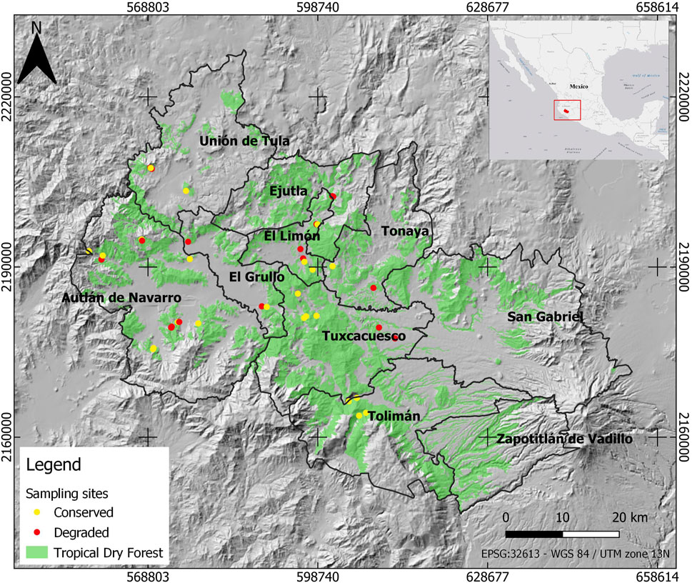
FIGURE 1. The study area location. The yellow and red dots indicate forest survey plots and the black lines represent the boundaries of the municipalities. The area of tropical dry forests was delimited by visual interpretation of Landsat images of 2018. The map was projected to UTM 13N WGS84.

3 Materials and Methods

As shown in Figure 2, the methods are composed of the following major steps: 1) spatial data processing. In this step, satellite images of both Landsat-8 and Sentinel-2 were obtained and based on which, various spectral indices and texture metrics were calculated; 2) field data measurement. In this step, the obtained field sampling data were processed and compared; 3) forest attributes mapping, and 4) degraded forest mapping and biophysical and socio-economic variables identification. In these two steps, forest attributes data were mapped using regression models and degraded forest was characterized based on maps of forest attributes and field measurement data. The most relevant biophysical and socio-economic factors to degraded forest were also identified.

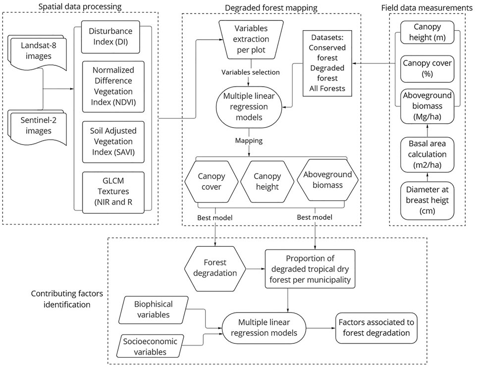
FIGURE 2. Diagram of the general methodology.

3.1 Field Data Sampling and Forest Survey Data Collection

The field data were collected from 28 May to 5 June 2019, which corresponds to the end of the dry season and the beginning of the rainy season. Affected by seasonality, tropical dry forests lose most of their leaves during the dry season, and they respond rapidly to the onset of the rainy season with fast greening. The location of the sample plots was decided by visually analyzing Landsat time series images from 2016 to 2018, together with high spatial resolution images from Google Earth. Initially, 60 locations in tropical dry forest were selected including both degraded and conserved forest with 30 points for each type of forest. Degraded forest locations were defined as areas that showed visible changes in the image texture while conserved forest showed no change. Later, these points were adjusted with expert knowledge regarding accessibility and safety as well as forest conditions. The final data included 41 sampling plots, with 23 plots of conserved forest and 18 plots of degraded forest.

Each sampling plot covers a circular area of 500 m², divided into a central area of 30 m², in which all trees with a diameter at breast height (DBH, breast height = 1.30 m) above 2.5 cm were measured, and a peripheral part in which only those trees with a DBH above 5 cm were measured. For each sampled tree, its canopy height, DBH and the number of branches were registered. Additionally, the percentage of canopy cover of each plot was measured using a concave spherical ground densiometer. Afterward, each plot’s mean canopy height was calculated as the average of the individual tree heights within the plot, while basal area and the number of branches corresponded to the sum of the individual measures. In turn, density of trees was calculated based on the number of trees registered for each plot. The aboveground biomass (AGB) for each tree was calculated using an allometric equation (Eq. 1) developed for tropical dry forest in the coastal area of Biosphere Reserve Chamela-Cuixmala, Jalisco (Martinez-Yrizar et al., 1992) which is about 60 km away from the study area.

In which log10 is the logarithm (base 10), AGB stands for aboveground biomass in Kg, A is a constant (−0.5352), and BA is the basal area in cm² of each sampled tree. Then, the individual AGB for each tree were summed to obtain the AGB by plot. Finally, all the forest attributes affected by area (i.e., basal area, AGB, number of branches, density of trees and density of branches) were extrapolated to 1 ha. Thus, the TDF attributes for each plot consisted of canopy cover (%), canopy height (m), basal area (m²/ha), AGB (Mg/ha), density of branches (№/ha), and density of trees (№/ha).

3.2 Remote Sensing Data

Remote sensing data come from two sensors, Landsat-8 and Sentinel-2. Landsat-8 (L8) OLI from collection level-1 was obtained from NASA Earth Explorer (www.earthexplorer.com) with acquisition dates ranging from 01 May 2019, to 29 July 2019, covering both dry and rainy seasons, which also corresponding to the timing of the field sampling data. This level-1 product was already geometrically corrected and orthorectified with a digital elevation model to correct for topography effects. It was also radiometrically calibrated at the top of the atmosphere level and therefore, we applied the Dark Object Subtraction method (Chavez 1986) to obtain the image at surface reflectance level. Sentinel-2 (S2) images with ates ranging from 18 April 2019 to 02 June 2019, at level 2A were also obtained. Level 2A products consist of geometrically and atmospherically corrected images at surface reflectance level, thus, no further correction was needed. The spectral bands of S2 images come with a spatial resolution of 10, 20, and 60 m and we only used the three visible bands and one near infrared band that have a spatial resolution of 10 m. The images from April and May were classified as data of the dry season, while the ones from June and July, as data of the rainy season. The selected Landsat-8 and Sentinel-2 images were acquired on different dates because we prioritized those with less cloud cover. Nevertheless, the difference in the date of acquisition was less than 2 months. Landsat images in the acquisition dates were cloud free and we created cloud masks using QA60 band for Sentinel-2 images. The atmospheric correction was carried out in QGIS (QGIS development team, 2019) and the cloud masks were obtained from Google Earth Engine (Gorelick et al., 2017).

3.2.1 Spectral Indices

To map forest attributes and to characterize area of degraded forest, we calculated spectral indices of the Normalized Difference Vegetation Index (NDVI), and Soil-adjusted vegetation index (SAVI) from the near infrared (NIR) and red (RED) bands of both L8 and S2 images in both dry and rainy seasons (Eqs 2, 3).

where the RED and NIR are band 4 (0.630–0.680 µm) and band 5 (0.845–0.885 µm), respectively, of L8 OLI, and band 4 (0.65–0.68 µm) and band 8 (0.78–0.90 µm), respectively, of S2. $L$ is a constant for adjusting influences from soil brightness, here we adopted the value of 0.5 for intermediate vegetation density (Huete, 1988).

In addition, for each Landsat and Sentinel image, we applied the Tasseled Cap (TC) transformation which reduces the dimensionality of the optical sensor’s spectral bands into three orthogonal indices of brightness, greenness, and wetness, calculated as weighted sums of the spectral bands. The design of the TC transformation specifically emphasizes inherent data structures that capture key physical properties of vegetated systems that can be compared both within and across scenes (Crist and Kauth 1986). TC brightness generally captures variation in overall reflectance; TC greenness captures variability in green vegetation, and it is a contrast of near infrared band and the visible bands; and TC wetness responds to a combination of moisture conditions and vegetation structure, and it is contrast of short-wave infrared bands with the other spectral bands (Cohen and Spies, 1992). We calculated these TC indices for each pixel using the band weightings provided by Baig et al. (2014) for L8 bands and for the bands of S2 images we used the weights given by Henrich et al. (2012). Finally, we computed a disturbance index (DI, Eq. 4), which is a linear combination of the components from a Tasseled Cap transformation of brightness, greenness and wetness (Healey et al., 2005).

where $B_r$ for brightness, $G_r$ for greenness and $W_r$ for wetness are rescaled Tasseled Cap transformations from 0 to 1.

3.2.2 Texture Data

Since texture metrics such as GLCM are important to map forest attributes and characterize degraded forest, we also calculated six texture metrics from the NIR and RED bands of the L8 and S2 images of both dry and rainy seasons with the method of Gray Level Co-occurrence Matrix (GLCM) including mean, variance, entropy, dissimilarity, homogeneity, and contrast (Haralick et al., 1973; Haralick 1979). These metrics were calculated using 64 levels of gray, an offset = 1 pixel and averaging the values in the four possible directions (0°, 90°, 180°, and 270°) with a window size of 3 by 3.

3.2.3 Image Variables Extraction and Selection

We used regression model to map forest attributes and characterize degraded forest. To extract spectral variables for each sample plot, first, we created a buffer area with a radius of 12.6 m around the center of each plot to cover the sampling area, and then we extracted the pixels of the spectral variables that intersected with this area. We calculated the mean values for the areas where there were multiple pixels in one buffer area. For the regression model, we obtained 12 spectral indices resulting from a combination of the three spectral indices (NDVI, SAVI, and DI), the two seasons (dry and rainy season), and the two types of images (L8 and S2). We also obtained 48 texture metrics from a combination of the six GLCM texture metrics, the two seasons (dry and rainy season), the two images (L8 and S2) and the two spectral bands (NIR and R). Additionally, we obtained one slope variable from a Digital Elevation Model with 15 m spatial resolution.

3.3 Forest Structural Attributes Modeling

We used multiple linear regression (MLR) by ordinary least squares (OLS) to find out which image variables can help predict forest structural attributes as measured in the ground-level forest survey. The response variables in the regression model are canopy cover, canopy height, and AGB. The explanatory variables include the above mentioned 12 spectral indices, 48 texture metrics, and one slope variable. We excluded the explanatory variables that are highly intercorrelated and included only variables that have an inter-correlation coefficient (Pearson) lower than 0.8.

Because we have a reduced number of plots, we limited the number of explanatory variables in the MLR to three. The MLR models include from one to three explanatory variables without interaction (Eqs 5–7) and one model that includes two explanatory variables and their interaction (Eq. 8).

Model with one explanatory variable. $y$ is the response variable, $x_1$ is the explanatory variable, $b_1$ is the slope coefficient, and $b_0$ is the y intercept when x = 0.

Model with two explanatory variables. $y$ is the response variable, $x_1, x_2$ are the explanatory variables, $b_1$ is the slope coefficient, and $b_0$ is the y intercept when x = 0.

Model with three explanatory variables. $y$ is the response variable, $x_1, x_2$, $x_3$ are the explanatory variables, $b_1$ is the slope coefficient, and $b_0$ is the y intercept when x = 0.

Model with two explanatory variables and their interaction. where $y$ is the response variable, $b_0$ is the y intercept when x = 0, $x_1$, $x_2$ are explanatory variables and $b_1$, $b_2,b_3$ are slope coefficients for each explanatory variable and for the interaction of the two explanatory variables, $x_1{x}_2$ (Eq. 8).

]We fitted the regression models to three forest types: 1) all-forest, that is, including both degraded and conserved forest samples; 2) degraded forest, and 3) conserved forest. After eliminating highly correlated explanatory variables, 23 variables were used for all-forest models, and 20 variables for each of the conserved and degraded forest models. The model performance was determined by its coefficient of determination (R²) and the corrected Akaike Information Criteria (AICc). A better model is characterized by a higher R² and a lower AICc. When comparing models with the same independent variables, the one with higher R² was chosen as the best, while comparing models with a different number of parameters, the one with lower AICc was chosen as the best. If two or more models showed an AICc difference of less than 2 units, the simplest model (with fewer variables) was chosen as the best (Burnham and Anderson 2002). We used “leave-one-out” cross validation to validate the model. This method generates a set of validation data by randomly leaving out one sample of the dataset.

3.3.1 Mapping Forest Degradation

A previous analysis using the same field survey data showed that only three forest structure attributes (canopy cover, canopy height, and AGB) were significantly different between degraded and conserved forest, by a Wilcoxon test (Table 1; Gao et al., 2020b). Thus, only the best models of these three attributes were used to construct the maps of degraded forest. We classified TDF into degraded and conserved forest using thresholds of forest attributes defined by a logistic regression in the above-mentioned study, achieving an overall accuracy of 72.22%–80.56% (Gao et al., 2020b). For AGB, the threshold is 27.5 Mg/ha, for canopy cover it is 90.9% and for canopy height it is 5.3 m (Gao et al., 2020b).

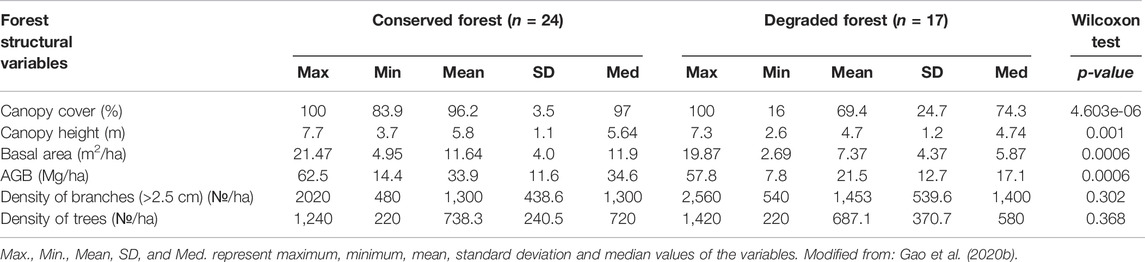
TABLE 1. Summary of forest structural variables in conserved and degraded forest obtained from field measurements during the dry season.

As mentioned, there were three models by forest type, i.e., all-forest, conserved and degraded forest. We first classified the attribute maps into binary images, where class one represented the attribute values below the thresholds (i.e., degraded forest), and class zero, the attribute values above the thresholds (i.e., conserved forest). Then, we summed the three maps and defined the final degraded forest area as that showing the three attributes in a degraded condition. After visually inspecting these results, we considered that the degraded forest model best depicted the actual forest conditions in the study area, and it was chosen to map the degraded forest. A forest mask made by visual interpretation using Landsat-8 images of 2018 was applied to exclude areas that did not correspond to TDF. We computed the area of degraded forest and calculated the ratio of degraded forest to the total area of TDF in each municipality.

3.4 Biophysical and Socioeconomic Variables Associated With Forest Degradation

After obtaining the degraded forest maps, we compiled several biophysical and socioeconomic variables that could help explain the percentage of degraded forest by municipality. We considered three biophysical variables including distance from settlements to forest (dist-TDF-settlements), distance from roads to forest (dist-TDF-roads), and slope. The first two variables were calculated using human settlements and road layers obtained from the Mexican National Institute of Statistics and Geography (Instituto Nacional de Estadística, Geografía (INEGI), 2016; Instituto Nacional de Estadística, Geografía (INEGI), 2021). Both dist-TDF-settlements and dist-TDF-roads were calculated based on the nearest linear distance from each settlement or road to the boundary of TDF, and they were averaged by each municipality. Slope was obtained in degrees from a digital elevation model with a 15-m resolution and also averaged by municipality. Based on previous studies, we hypothesized that municipalities with forest closer to roads and settlements and with lower slope should have a higher percentage of degraded forests, since they were more accessible (Morales-Barquero et al., 2015; Borrego and Skutsch 2019; Guerra-Martínez et al., 2019).

For socio-economic variables, we considered the land tenure within each municipality, expressed as the percentage of land that is under the social ownership (ejido property), according to the National Agrary Record (Registro Agrario Nacional (RAN), 2022). We also considered the percentage of parceled and communal-use lands, since ejido property is composed of both. The spatial distribution of ejido, parceled land and communal-use areas within municipalities is presented in Supplementary Figure S1. We also considered a poverty index (Consejo Nacional de Población (CONAPO), 2020) with higher values corresponding to greater poverty. The demographic data of each municipality (Instituto Nacional de Estadística, Geografía (INEGI), 2020) and production data of both crop agriculture and cattle ranching were also included. We computed the agricultural and livestock production in units of Mg per ha averaged between 2017 and 2019 with the data extracted from the department of agriculture and rural development (SIAP, 2022). We also included the data on firewood consumption at the municipal level in 2008 (Pacheco et al., 2008). Although this data is not up to date, we believe that firewood use has not changed significantly in the intervening period. Based on previous studies, we expected that municipalities with a higher percentage of land under social ownership, less poverty, less population, less agriculture, and cattle production, as well as less firewood consumption, should correspond to those with less percentage of degraded forest (Morales-Barquero et al., 2015; Borrego and Skutsch 2019; Guerra-Martínez et al., 2019). The complete biophysical and socio-economic variables were listed in Supplementary Table S1.

3.5 Forest Degradation Models

We used multiple linear regression (see Section 3.3) to identify the most relevant biophysical and socio-economic factors that are associated with forest degradation at municipality level (see Section 3.3.1). In these models, the percentage of degraded forest with respect to the total forest area was the dependent variable, while the three biophysical and eleven socioeconomic variables were used as independent variables. To eliminate highly inter-correlated independent variables, we removed the variables that had a Pearson correlation coefficient above 0.8. After this procedure, two biophysical variables (distance to settlements and slope) and nine socioeconomic variables (percentage of municipality under parceled land regime, percentage of municipality under communal-use ownership, poverty index, fuelwood consumption, temporal agriculture production, irrigated agriculture production, percentage of forest under parceled land regime, percentage of forest under communal-use ownership) were used as explanatory variables.

The vegetation indices, texture metrics calculation and all statistical procedures and models were carried out in R (R Core Team, 2021). The satellite images processing was carried out in QGIS (QGIS development team, 2019).

4 Results

4.1 Forest Attributes Modeling With Remote Sensing Data

4.1.1 Best Model Selection

The best models for the three forest attributes that were significantly different between degraded and conserved forest, that is, canopy cover, canopy height, and AGB were selected for the models fitted with the all-forest, conserved forest, and degraded forest datasets (Table 2). The model goodness-of-fit (R²) was consistently higher in the degraded forest model, followed by the conserved forest model, and then by the all-forest model. In the degraded forest model, the R² was higher than 0.62 for the three forest attributes, which means that the spectral variables in these models can explain at least 62% of the variation in the forest attributes.

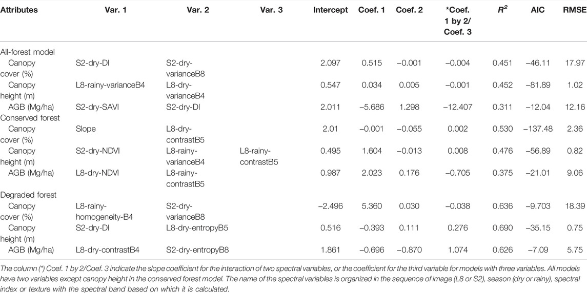
TABLE 2. Best models for all-forest, conserved forest, and degraded forest.

4.1.2 Model Validation, Observed vs. Predicted

By “leave-one-out” cross validation (CV), using the model of degraded forest, the model for AGB had the best CV result ($R_{cv}^2$ = 0.53), followed by canopy height ($R_{cv}^2$ = 0.46), and then by canopy cover ($R_{cv}^2$ = 0.36). Using the all-forest model, the goodness-of-fit from the CV procedure is $R_{cv}^2$ = 0.16 for AGB, $R_{cv}^2$ = 0.012 for Canopy cover and $R_{cv}^2$ = 0.32 for canopy height. With the conserved forest model, the canopy height had a goodness-of-fit of $R_{cv}^2$ = 0.18, canopy cover of $R_{cv}^2$ = 0.17, and AGB, $R_{cv}^2$ = 0.08. Compared with the degraded forest model, the all-forest model and the conserved forest model have reduced their predictive power with a leave-one-out dataset, with evidently much lower $R_{cv}^2$ values. Furthermore, this observation gave us an additional reason for selecting the degraded forest model as the one used in forest degradation mapping. Using the models presented in Table 2, the forest attributes were predicted and compared with the observed attributes (Figure 3). In this figure, one would expect a slope = 1, and R² = 1 for perfectly fitted models. In addition, among the constructed models, the ones that showed a better goodness-of-fit are the degraded forest models.

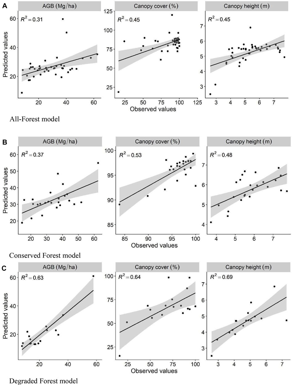
FIGURE 3. Predicted vs. observed forest attributes with the best models of different datasets. The gray areas show the confidence intervals. (A): all-forest dataset; (B): conserved forest dataset; (C): degraded forest dataset.

4.2 Mapping Forest Degradation

We mapped the forest attributes of canopy cover, canopy height and AGB using the best models of all three model types (degraded forest model, conserved forest model, and all-forest model). The maps (Figure 4) indicate that forest area with value zero has all three attributes in a conserved status; forest area with value one has one attribute that falls into the degraded category; areas with value two have two such attributes, and areas with value three have all three forest attributes in the degraded category. In the map produced by the conserved forest model, most of the forest area is in a conserved state, and there is only 1.86% of forest area in a degraded category, which is equivalent to 2,348.20 ha. In the map using all-forest model 15.33% of forest, 19,317.71 ha, is in a degraded category, and in the map produced from the degraded forest model, degraded forest dominates with 49.91% of the area, covering 62,878 ha. Considering the history of the intensive use of the tropical dry forest for shifting cultivation, cattle grazing, and fuelwood collection in the study area, we adopt the result of the degraded forest model to study the associated biophysical and socio-economic factors.

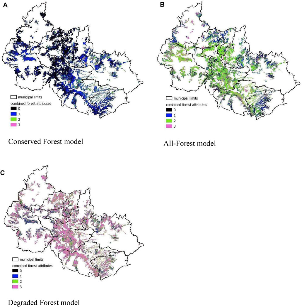
FIGURE 4. Maps indicating the sum of the number of structural attributes (canopy cover, canopy height and AGB) below the degraded threshold and produced by (A) the Conserved Forest model, (B) All-Forest model, and (C) Degraded Forest model, respectively.

4.3 The Biophysical and Socio-Economic Variables That Are Associated With Forest Degradation

The best model to describe the percentage of degraded forest over the total area of forest by its biophysical and socio-economic variables is summarized in Table 3.

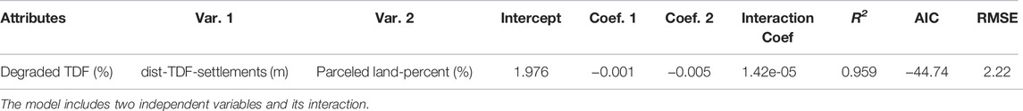
TABLE 3. Best model for degraded forest expressed as the percentage of degraded forests in each municipality.

The percentage of degraded forest in each municipality is best explained by distance to settlements (dist-TDF-settlements) and percentage of forest in parceled land, with negative coefficients for both variables, but a positive coefficient for its interaction (Table 3). These two variables can explain 95.8% of the variance in the percentage of degraded forest. According to this model, the municipalities where the forests are closer to the settlements have higher percentages of degraded forest, while municipalities with a higher percentage under parceled land ownership have a lower percentage of degraded forest. However, its interaction has a positive coefficient, meaning that municipalities where the forest is farthest from settlements and with a higher land tenure under parceled land, tend to have a higher percentage of degraded forest.

Figure 5 shows the spatialized factors associated with forest degradation, as well as the remaining forest area. This figure shows that the municipalities with the highest percentage of degraded forest are located in the center of the ARB, while the ones with the largest remaining tropical dry forest areas can be found in the southern part of the ARB. Additionally, the municipalities with the lowest remaining forest cover are El Limón and El Grullo, which are also the smallest municipalities in the ARB.

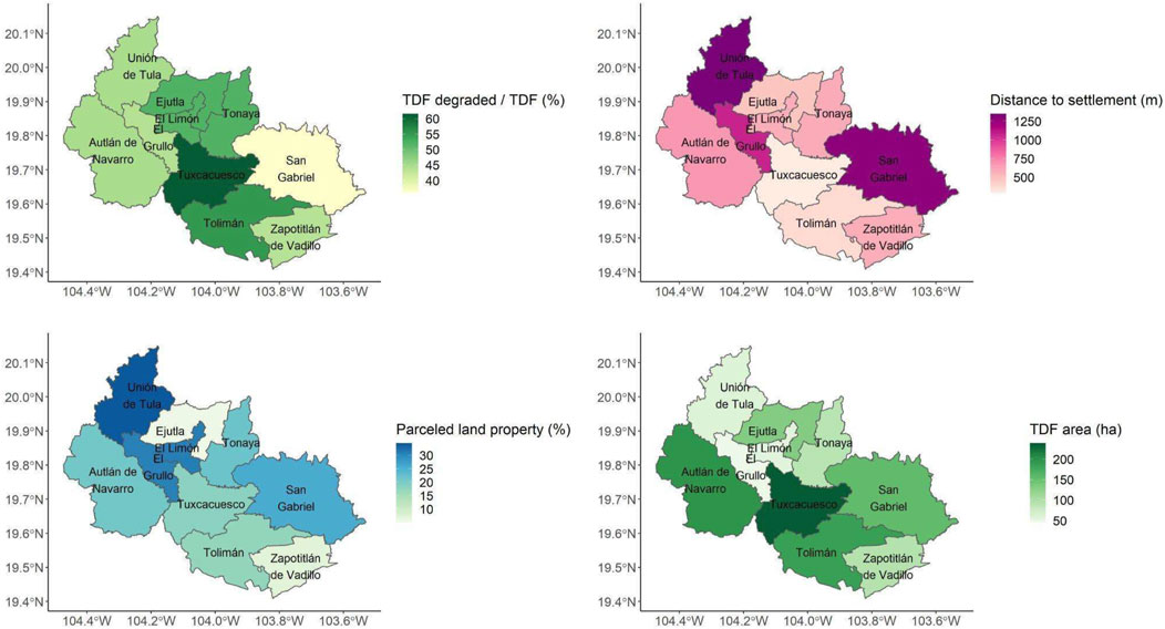
FIGURE 5. The mapped degraded forest and the two biophysical and socio-economic factors relevant to explain the percentage of degraded forest by municipality.

5 Discussion

5.1 Mapping Forest Attributes Using Remote Sensing and Field Inventory Data

Three different types of models were fitted according to the forest degradation status, i.e., degraded, conserved and both (i.e., all-forest). However, since each one was constructed with different subsets of the same data, they differ in the variables included, as well as in their goodness-of-fit (R²). The higher R² value shown by the degraded forest model might be related to the fact that there is more variation that can be modeled by the image metrics, in comparison with the conserved forest. For example, previous studies have reported that models of old-growth forest attributes often show lower R² values than models of secondary forests, which can be considered as forming a gradient of degraded forests (Eckert, 2012; Gallardo-Cruz et al., 2012; Solórzano et al., 2017). Additionally, several of these studies created their secondary forest datasets according to a successional stage gradient, which ensures that the dataset is heterogeneous and covers a wide variety of structural attribute values. On the contrary, in the studies focused on old-growth forests, there is no evident gradient that can maximize heterogeneity and admittedly, structural heterogeneity in old-growth forests is far less than that of secondary forests with different ages of abandonment.

Although at a first glance, the all-forest dataset could represent a “middle point” model, it showed most of the forest as non-degraded (value = 2; Figure 3), which we considered did not accurately represent the forest condition in the ARB. Furthermore, because the degraded forest models showed higher R² and R_CV² values we considered it a better model to identify degraded forest in the study area. We suspect that the all-forest models showed lower goodness-of-fit, in comparison to the degraded forest ones, because the forest attribute—image variables relationship showed a non-linear pattern in that dataset. Thus, we chose the degraded forest model to map the degradation in the ARB. Finally, we could have classified forest degradation according to each forest attribute (i.e., AGB, canopy cover and mean height); however, we used a conservative approach to define degraded forest, that is, degraded forest was defined as forest with lower values on all three forest structural variables.

In our work, the DI derived from the Sentinel-2 images, in combination with the Landsat-8 entropy metric had a good response in detecting canopy height (R² = 0.69). Both metrics are possibly complementary, but the DI indicates a good response of degradation associated with decreasing height. Previously DI has been derived from coarser spatial resolution images such as Landsat and MODIS and used for disturbance detection from agriculture and fires (Masek et al., 2008; Hilker et al., 2009). In this work, Sentinel-2 derived DI contributed to the model fitting possibly because of its higher spatial resolution. The use of a combination of images from different seasons could improve the identification of vegetation characteristics represented by vegetation structural variables. In the rainy season, the image variables are mostly associated with canopy cover characteristics; thus, we expected higher predictive power from this set of variables. However, the dry season images turned out to be better explanatory variables for the canopy height and AGB parameters of the degraded forest dataset. A possible explanation could be that during the dry season, tropical dry forests lose most of their foliage, and thus, the images capture reflectances from branches, trunks and dry leaves or soil (Ferreira and Huete, 2004).

There was a large presence of textural metrics in our models. These metrics have been shown to explain the variation of structural attributes in tropical dry forest (Gallardo-Cruz et al., 2012; Barbosa et al., 2014; Solórzano et al., 2017). Our models showed that the textural metrics of variance, contrast, entropy, and homogeneity explained variations in most of the vegetation attributes. Texture metrics have been shown to be associated with vegetation homogeneity or heterogeneity characteristics, i.e., in continuous uniform areas of conserved forest, the contrast between pixel tones is usually lower. While in disturbed areas, the images will capture not only canopy characteristics, but also fragments of trunks, branches and soil that are exposed by vegetation disturbances, which usually increases the values of textures measuring heterogeneity.

5.2 Mapping Forest Degradation

We estimated that 49.9% of the tropical dry forest in the study area is degraded, using the criterion of canopy cover less than 90.9%, AGB less than 27.5 Mg/ha and canopy height lower than 5.3 m. Most of these areas were located at the boundaries with other land use, such as agriculture, where they coincide with the fragmented forests. At the edges of these fragments, the forests are usually composed of trees of lower height, smaller basal area and lower biomass due to an “edge effect” from the mortality of large trees caused by land clearing for agricultural activity (Almeida et al., 2019). This effect may also come from the alteration in the microclimate and therefore, those trees that do not tolerate the stress of high temperatures and lower humidity may gradually die (Laurance et al., 2007). In addition, an activity frequently seen in the field, especially in degraded forests, is the presence of cattle that graze freely within the forest, which worsens the situation of the forest’s border areas. One of the important effects of grazing in forests is the high mortality of young trees, which reduces tree recruitment and hinders forest recovery and carbon storage, especially of those species that have the greatest potential to accumulate carbon (Chaturvedi et al., 2012). Therefore, constant livestock activity could be one of the fundamental causes of forest degradation in this region. In Section 5.4, we will further elaborate on the effects of cattle grazing as socio-economic factors for forest degradation.

Previous studies suggested that most of the tropical dry forest in the study area is in a degraded state (Salinas-Melgoza et al., 2017), which partially agrees with our findings. However, studies also showed that the AGB of the tropical dry forests also corresponds to topography variables by combining anthropogenic and biophysical factors (Salinas-Melgoza et al., 2018). Therefore, a limitation in our work is that natural forests with low AGB, canopy cover, or canopy height were probably classified as degraded forests. Therefore, we need to consider the elevation and slope thresholds to refine our degraded forest map, implying a much larger dataset acquisition. Limited by time and monetary cost, we opt to leave this for future work. Nevertheless, verification of our degraded forest maps will still be needed to assess the precision of the adopted approach.

5.3 Socio-Economic and Biophysical Factors Associated With Forest Degradation

The most relevant socio-economic and biophysical variables to explain the percentage of degraded forest by municipality were distance to settlements and percentage of land under parceled land property. Together they explained more than 95% of the variance in degraded forest by municipality (%). Previous studies have reported similar findings. For example, Morales-Barquero et al. (2015) reported that in the same study area, the factors most related to forest degradation were marginalization, forest area/population ratio, use of forest as a source of posts, livestock management and slope. Additionally, Corona-Núñez et al., 2021 found that distance to agricultural areas, settlements and dirt roads, as well as elevation, are among the factors related to tropical dry forest biomass reduction in the Mexican Pacific Coast. In turn, Vaca et al. (2019) found that accessibility related factors, slope, and land tenure were among the principal factors explaining deforested areas in Southeast Mexico.

In our study, the variables of distance to settlements, cattle production and distance to roads were strongly correlated (r >= 0.82), thus, the last two variables were removed from the analysis. Therefore, we cannot conclude, for example, that cattle production was not an important factor to explain the percentage of degraded forest by municipality, but rather that any one of these three variables might act as explanatory variables with similar predictive power. In fact, according to the field observations, cattle production might play an important role in forest degradation, as well as the distance to roads, as an indicator of accessibility. In the case of the percentage of parceled land, the only highly correlated variable was the percentage of ejido property (r = 0.82), which contains both parceled land and communal-use land. In this case, we consider that the percentage of ejido property is a variable with similar predicting power as the percentage of parceled land and might be a better indicator to explain the percentage of degraded forest (Supplementary Figure S2).

5.4 Limitations and Future Work

We focused on testing the explanatory power of biophysical and socio-economic factors only for the percentage of degraded forest. However, these factors could be valuable to explain other unmeasured variables such as percentage of remaining forest cover which is associated with deforestation in the study area. This study focused on forest degradation, however, in order to get a complete picture of forest transformation and the use of forest resources in the region, the area of transformed forest to agricultural or pastureland should also be accounted for. For example, it is interesting that Figure 4 shows that Tuxcacuesco is the municipality with the highest percentage of degraded forest and also, the one with the largest extent of remaining forest. Finally, the same factors that are relevant for forest degradation could also be related to deforestation in the region.

Admittedly, other biophysical and socio-economic factors could be important to help explain the percentage of degraded forests, for example, the number of livestock, the percentage of inhabitants dedicated to cattle ranching or agricultural activities, the use of forest for activities such as constructing fences, cattle grazing, or medicinal plants. All these activities contribute to forest degradation; however, the data was either not updated or not available at municipal level.

Due to logistics and accessibility constraints, we did not cover all important forest sampling sites during field surveys, which might affect the modeling result of forest status. On the other hand, the modeling of forest attributes could be limited by the spatial resolution of satellite images. We used images with spatial resolution of up to 10 m, but degradation could occur in smaller areas. To have more precise information on the level of degradation and forest status, it is important to consider images with higher spatial resolutions.

In addition, the forest structural information can be better captured by L- or P-band SAR, airborne LiDAR or GEDI data (Dupuis et al., 2020). With these last considerations, it would be possible to include information on canopy height or branch density in the models. The incorporation of auxiliary variables such as soil erosion, soil moisture, management history, among others, can be used to characterize degraded forest. This, together with higher resolution satellite images, can better characterize forest conditions.

Uncertainty analysis in biomass estimation with remote sensing is often hampered by the difficulty in obtaining reference data. Major error components often include the sampling error, measurement error for diameter, and regression error for tree biomass from different allometric equations (Phillips et al., 2000). When remote sensing data is used, the error sources can extend to data processing techniques and input parameters in modeling algorithms (Lu et al., 2012). Compared with the case study in Lu et al. (2012) which estimated biomass using Landsat TM and Lidar with the dominant uncertainty sources in sample plot data and optical sensor saturation problem, our study integrated the strengths of multi-sensor data and texture metrics and therefore increased the confidence in forest biomass estimates.

6 Conclusion

We presented an approach to map degraded forests in the Ayuquila River Basin, Jalisco, Mexico. Our results showed that 49.91% of the remaining forest in the study site was degraded, covering 62,878 ha. We used a regression model to map forest structural attributes, including AGB, canopy cover, and canopy height, with spectral indices and texture metrics derived from Landsat-8 and Sentinel-2 images. We then identified degraded forests as those areas that fall under a discrimination threshold between the degraded and conserved forests. We found that texture variables were essential in modeling forest attributes, especially the metrics measured in the dry season when tropical dry forests lose their leaves. As for the underlying biophysical and socioeconomic factors associated with forest degradation, we found that distance from settlements and parceled land ownership explained the most variation in the degraded forest by municipalities. Both factors showed a positive trend with degraded forest. Future studies should evaluate the precision of our degraded forest map and test which socioeconomic and biophysical factors explain forest degradation at a much finer scale. Finally, due to the large proportion of degraded forests in the study area, we suggest that future policy interventions are directed towards more sustainable use of the forests to promote forest conservation.

Data Availability Statement

The original contributions presented in the study are included in the article/Supplementary Material, further inquiries can be directed to the corresponding author.

Author Contributions

YG, DLJ-R, and JVS contributed to conceptualization; JVS, DLJ-R, and YG contributed to methodology and data curation; YG, JVS, and DLJ-R contributed to the writing of the first draft; MS, MAS-M, DRP-S, and MF contributed to the editing of the first draft. All authors agreed to the submission of the final version.

Funding

This work was funded by the Consejo Nacional de Ciencia y Tecnología (CONACyT), “Ciencia Básica” SEP-285349.

Conflict of Interest

The authors declare that the research was conducted in the absence of any commercial or financial relationships that could be construed as a potential conflict of interest.

Publisher’s Note

All claims expressed in this article are solely those of the authors and do not necessarily represent those of their affiliated organizations, or those of the publisher, the editors and the reviewers. Any product that may be evaluated in this article, or claim that may be made by its manufacturer, is not guaranteed or endorsed by the publisher.

Acknowledgments

The authors would like to acknowledge Samuel and Oscar Ponce from Junta Intermunicipal de Medio Ambiente para la gestión de la Cuenca Baja del Río Ayuquila (JIRA) for their valuable advice during the fieldwork. Thanks also go to Jaime Loya, Ernesto Carrillo, Miriam San Jose and Rita Adame for their assistance and participation in the fieldwork.

Supplementary Material

The Supplementary Material for this article can be found online at: https://www.frontiersin.org/articles/10.3389/fenvs.2022.912873/full#supplementary-material

References

Almeida, D. R. A., Stark, S. C., Schietti, J., Camargo, J. L. C., Amazonas, N. T., Gorgens, E. B., et al. (2019). Persistent Effects of Fragmentation on Tropical Rainforest Canopy Structure after 20 Yr of Isolation. Ecol. Appl. 29, e01952. doi:10.1002/eap.1952
Asner, G. P., Powell, G. V., Mascaro, J., Knapp, D. E., Clark, J. K., Jacobson, J., et al. (2010). High-resolution Forest Carbon Stocks and Emissions in the Amazon. Proc. Natl. Acad. Sci. U. S. A. 107, 16738–16742. www.pnas.org/cgi/doi/10.1073/pnas.1004875107. doi:10.1073/pnas.1004875107
Baig, M. H. A., Zhang, L., Shuai, T., and Tong, Q. (2014). Derivation of a Tasseled Cap Transformation Based on Landsat 8 At-Satellite Reflectance. Remote Sens. Lett. 5, 5. doi:10.1080/2150704x.2014.915434
Barbosa, J. M., Broadbent, E. N., and Bitencourt, M. D. (2014). Remote Sensing of Aboveground Biomass in Tropical Secondary Forests: A Review. Int. J. For. Res. 2014, 1–14. doi:10.1155/2014/715796
Berenguer, E., Ferreira, J., Gardner, T. A., Aragão, L. E. O. C., De Camargo, P. B., Cerri, C. E., et al. (2014). A Large-Scale Field Assessment of Carbon Stocks in Human-Modified Tropical Forests. Glob. Change Biol. 20, 3713–3726. doi:10.1111/gcb.12627
Bonilla-Moheno, M., Aide, T. M., and Clark, M. L. (2012). The Influence of Socioeconomic, Environmental, and Demographic Factors on Municipality-Scale Land-Cover Change in Mexico. Reg. Environ. Change 12, 543–557. doi:10.1007/s10113-011-0268-z
Borrego, A., and Skutsch, M. (2019). How Socio-Economic Differences between Farmers Affect Forest Degradation in Western Mexico. Forests 10, 893. doi:10.3390/f10100893
Burnham, K. P., and Anderson, D. R. (2002). Model Selection and Multimodel Inference: A Practical Information-Theoretic Approach. New York: Springer.
Caughlin, T. T., Barber, C., Asner, G. P., Glenn, N. F., Bohlman, S. A., and Wilson, C. H. (2021). Monitoring Tropical Forest Succession at Landscape Scales Despite Uncertainty in Landsat Time Series. Ecol. Appl. 31, e02208. doi:10.1002/eap.2208
Challenger, A., and Soberón, J. (2008). Los ecosistemas terrestres, en Capital natural de México, I. México: Conocimiento actual de la biodiversidad. Conabio.
Chaplin-Kramer, R., Sharp, R. P., Mandle, L., Sim, S., Johnson, J., Butnar, I., et al. (2015). Spatial Patterns of Agricultural Expansion Determine Impacts on Biodiversity and Carbon Storage. Proc. Natl. Acad. Sci. U. S. A. 112, 7402–7407. doi:10.1073/pnas.1406485112
Chaturvedi, R. K., Raghubanshi, A. S., and Singh, J. S. (2012). Effect of Grazing and Harvesting on Diversity, Recruitment and Carbon Accumulation of Juvenile Trees in Tropical Dry Forests. For. Ecol. Manag. 284, 152–162. doi:10.1016/j.foreco.2012.07.053
Chavez, P. S. (1986). An Improved Dark-Object Subtraction Technique for Atmospheric Scattering Correction of Multispectral Data. Remote Sens. Environ. 24, 3. doi:10.1016/0034-4257(88)90019-3
Clark, M., and Tilman, D. (2017). Comparative Analysis of Environmental Impacts of Agricultural Production Systems, Agricultural Input Efficiency, and Food Choice. Environ. Res. Lett. 12, 6. doi:10.1088/1748-9326/aa6cd5
Cohen, W. B., and Spies, T. A. (1992). Estimating Structural Attributes of Douglas-Fir/Western Hemlock Forest Stands From Landsat and SPOT Imagery. Remote Sens. Environ. 41, 1–17. doi:10.1016/0034-4257(92)90056-P
CONABIO (2020). Selvas Secas. Available at: https://www.biodiversidad.gob.mx/ecosistemas/selvaSeca. (Accessed April 2, 2022)
Consejo Nacional de Población (CONAPO) (2020). Índice de marginación por entidad federativa y municipio 2020. Available at: https://www.gob.mx/conapo/documentos/indices-de-marginacion-2020-284372. (Accessed January 21, 2022)
Corona-Núñez, R. O., Mendoza-Ponce, A. V., and Campo, J. (2021). Assessment of Above-Ground Biomass and Carbon Loss from a Tropical Dry Forest in Mexico. J. Environ. Manag. 282, 111973. doi:10.1016/j.jenvman.2021.111973
Crist, E. P., and Kauth, R. J. (1986). The Tasseled Cap De-mystified. Photogrammetric Eng. Remote Sens. 52, 81–86.
Curtis, P. G., Slay, C. M., Harris, N. L., Tyukavina, A., and Hansen, M. C. (2018). Classifying Drivers of Global Forest Loss. Science 361, 1108–1111. doi:10.1126/science.aau3445
Das, S., and Singh, T. P. (2012). Correlation Analysis between Biomass and Spectral Vegetation Indices of Forest Ecosystem. IJERT 1, 1–13. doi:10.17577/IJERTV1IS5369
de la Barreda-Bautista, B., López-Caloca, A. A., Couturier, S., and Silván-Cárdenas, J. L. (2011). “Tropical Dry Forests in the Global Picture: The Challenge of Remote Sensing-Based Change Detection in Tropical Dry Environments,” in Planet Earth 2011 - Global Warming Challenges and Opportunities for Policy and Practice, Editor E. Carayannis (London, United Kingdom: TechOpen ), 231–256. doi:10.5772/24283
DeFries, R. S., Houghton, R. A., Hansen, M. C., Field, C. B., Skole, D., and Townshend, J. (2002). Carbon Emissions from Tropical Deforestation and Regrowth Based on Satellite Observations for the 1980s and 1990s. Proc. Natl. Acad. Sci. U. S. A. 99, 14256–14261. doi:10.1073/pnas.182560099
Dube, T., and Mutanga, O. (2015). Investigating the Robustness of the New Landsat-8 Operational Land Imager Derived Texture Metrics in Estimating Plantation Forest Aboveground Biomass in Resource Constrained Areas. ISPRS J. Photogrammetry Remote Sens. 108, 12–32. doi:10.1016/j.isprsjprs.2015.06.002
Dupuis, C., Lejeune, P., Michez, A., and Fayolle, A. (2020). How Can Remote Sensing Help Monitor Tropical Moist Forest Degradation? A Systematic Review. Remote Sens. 12, 1087. doi:10.3390/rs12071087
Eckert, S. (2012). Improved Forest Biomass and Carbon Estimations Using Texture Measures from WorldView-2 Satellite Data. Remote Sens. 4, 12. doi:10.3390/rs4040810
Food and Agriculture organization of the United Nations (FAO) (2020). Global Forest Resources Assessment 2020 – Key Findings. Rome. doi:10.4060/ca8753en
Farfán Gutiérrez, M., Rodríguez-Tapia, G., and Mas, J.-F. (2016). Análisis jerárquico de la intensidad de cambio de cobertura/uso de suelo y deforestación (2000-2008) en la Reserva de la Biosfera Sierra de Manantlán, México. Investig. Geográficas 89, 104.
Feeley, K. J., Gillespie, T. W., and Terborgh, J. W. (2005). The Utility of Spectral Indices from Landsat ETM+ for Measuring the Structure and Composition of Tropical Dry Forests1. Biotropica 37, 508–519. doi:10.1111/j.1744-7429.2005.00069.x
Ferreira, L. G., and Huete, A. R. (2004). Assessing the Seasonal Dynamics of the Brazilian Cerrado Vegetation through the Use of Spectral Vegetation Indices. Int. J. Remote Sens. 25, 1837–1860. doi:10.1080/0143116031000101530
Gallardo-Cruz, J. A., Meave, J. A., González, E. J., Lebrija-Trejos, E. E., Romero-Romero, M. A., Pérez-García, E. A., et al. (2012). Predicting Tropical Dry Forest Successional Attributes from Space: Is the Key Hidden in Image Texture? PLoS ONE 7, e30506. doi:10.1371/journal.pone.0030506
Gao, Y., Skutsch, M., Jiménez-Rodríguez, D. L., and Solórzano, J. V. (2020b). Identifying Variables to Discriminate between Conserved and Forest and to Quantify the Differences in Biomass. Forests 11, 9. doi:10.3390/f11091020
Gao, Y., Skutsch, M., Paneque-Gálvez, J., and Ghilardi, A. (2020a). Remote Sensing of Forest Degradation: A Review. Environ. Res. Lett. 15, 103001. doi:10.1088/1748-9326/abaad7
Goetz, S. J., Hansen, M., Houghton, R. A., Walker, W., Laporte, N., and Busch, J. (2015). Measurement and Monitoring Needs, Capabilities and Potential for Addressing Reduced Emissions from Deforestation and Forest Degradation under REDD+. Environ. Res. Lett. 10, 123001. doi:10.1088/1748-9326/10/12/123001
Gonzalez-Navarro, M. G. (1977). Las Tierras Ociosas. Hist. Mex. 26, 503–539. http://www.jstor.org/stable/25135573.
Gorelick, N., Hancher, M., Dixon, M., Ilyushchenko, S., Thau, D., and Moore, R. (2017). Google Earth Engine: Planetary-Scale Geospatial Analysis for Everyone. Remote Sens. Environ. 202, 18–27. doi:10.1016/j.rse.2017.06.031
Guerra-Martínez, F., García-Romero, A., Cruz-Mendoza, A., and Osorio-Olvera, L. (2019). Regional Analysis of Indirect Factors Affecting the Recovery, Degradation and Deforestation in the Tropical Dry Forests of Oaxaca, Mexico. Singap. J. Trop. Geogr. 40, 387–409. doi:10.1111/sjtg.12281
Halperin, J., LeMay, V., Coops, N., Verchot, L., Marshall, P., and Lochhead, K. (2016). Canopy Cover Estimation in Miombo Woodlands of Zambia: Comparison of Landsat 8 OLI versus RapidEye Imagery Using Parametric, Nonparametric, and Semiparametric Methods. Remote Sens. Environ. 179, 170–182. doi:10.1016/j.rse.2016.03.028
Hansen, M. C., Stehman, S. V., and Potapov, P. V. (2010). Quantification of Global Gross Forest Cover Loss. Proc. Natl. Acad. Sci. U.S.A. 107, 8650–8655. doi:10.1073/pnas.0912668107
Haralick, R. M., Shanmugam, K., and Dinstein, I. H. (1973). Textural Features for Image Classification. IEEE Trans. Syst. Man. Cybern. SMC-3, 610–621. doi:10.1109/tsmc.1973.4309314
Haralick, R. M. (1979). Statistical and Structural Approaches to Texture. Proc. IEEE 67, 786–804. doi:10.1109/proc.1979.11328
Healey, S., Cohen, W., Zhiqiang, Y., and Krankina, O. (2005). Comparison of Tasseled Cap-Based Landsat Data Structures for Use in Forest Disturbance Detection. Remote Sens. Environ. 97, 301–310. doi:10.1016/j.rse.2005.05.009
Henrich, V., Krauss, G., Götze, C., and Sandow, C. (2012). Index DataBase. A Database for Remote Sensing Indices. URL Available at: https://www.indexdatabase.de/info/credits.php (Accessed. December 4-5. 2012).
Hilker, T., Wulder, M. A., Coops, N. C., Linke, J., McDermid, G., Masek, J. G., et al. (2009). A New Data Fusion Model for High Spatial- and Temporal-Resolution Mapping of Forest Disturbance Based on Landsat and MODIS. Remote Sens. Environ. 113, 1613–1627. doi:10.1016/j.rse.2009.03.007
Huete, A. R. (1988). A Soil-Adjusted Vegetation Index (SAVI). Remote Sens. Environ. 25, 295–309. doi:10.1016/0034-4257(88)90106-X
Instituto Nacional de Estadística, Geografía (INEGI) (2016). Cartografía Geoestadística Urbana Y Rural Scale 1:50000. [Map].
Instituto Nacional de Estadística, Geografía (INEGI) (2021). Red Nacional de Caminos (RNC) scale 1:250000. [Map].
Instituto Nacional de Estadística, Geografía (INEGI) (2014). Soil Type Information Vector Dataset Scale 1:50000 Serie III. [Map].
Instituto Nacional de Estadística, Geografía (INEGI) (2020). Censos y Conteos de Población y Vivienda. Available at: https://www.inegi.org.mx/programas/ccpv/2020/ (Accessed January 21, 2022).
Kissinger, G., Herold, M., and de Sy, V. (2012). Drivers of Deforestation and Forest Degradation: A Synthesis Report for REDD+ Policymakers [WWW Document]. CIFOR. URL Available at: https://www.cifor.org/knowledge/publication/5167/(Accessed Feburary 4, 2022).
Laurance, W. F., Nascimento, H. E., Laurance, S. G., Andrade, A., Ewers, R. M., Harms, K. E., et al. (2007). Habitat Fragmentation, Variable Edge Effects, and the Landscape-Divergence Hypothesis. PLoS ONE 2, e1017. doi:10.1371/journal.pone.0001017
Lawrence, R. L., and Ripple, W. J. (1998). Comparisons Among Vegetation Indices and Bandwise Regression in a Highly Disturbed, Heterogeneous Landscape: Mount St. Helens, Washington. Remote Sens. Environ. 64, 91–102. doi:10.1016/s0034-4257(97)00171-5
Lieberman, D., Lieberman, M., Peralta, R., and Hartshorn, G. S. (1996). Tropical Forest Structure and Composition on a Large-Scale Altitudinal Gradient in Costa Rica. J. Ecol. 84, 137–152. doi:10.2307/2261350
Lu, D., Chen, Q., Wang, G., Moran, E., Batistella, M., Zhang, M., et al. (2012). Aboveground Forest Biomass Estimation with Landsat and LiDAR Data and Uncertainty Analysis of the Estimates. Int. J. For. Res. 2012, 1–16. doi:10.1155/2012/436537
Martinez-Yrizar, A., Sarukhan, J., Perez-Jimenez, A., Rincon, E., Maass, J. M., Solis-Magallanes, A., et al. (1992). Above-ground Phytomass of a Tropical Deciduous Forest on the Coast of Jalisco, México. J. Trop. Ecol. 8, 87–96. doi:10.1017/S0266467400006131
Masek, J. G., Huang, C., Wolfe, R., Cohen, W., Hall, F., Kutler, J., et al. (2008). North American Forest Disturbance Mapped from a Decadal Landsat Record. Remote Sens. Environ. 112, 2914–2926. doi:10.1016/j.rse.2008.02.010
Mitchell, A. L., Rosenqvist, A., and Mora, B. (2017). Current Remote Sensing Approaches to Monitoring Forest Degradation in Support of Countries Measurement, Reporting and Verification (MRV) Systems for REDD+. Carbon Balance Manage 12, 9. doi:10.1186/s13021-017-0078-9
Morales-Barquero, L., Borrego, A., Skutsch, M., Kleinn, C., and Healey, J. R. (2015). Identification and Quantification of Drivers of Forest Degradation in Tropical Dry Forests: A Case Study in Western Mexico. Land Use Policy 49, 296–309. doi:10.1016/j.landusepol.2015.07.006
Pacheco, C., Ghilardi, A., Guerrero, G., Masera, O., Carrillo, U., Castellarini, F., et al. (2008). Balance Entre Oferta y Consumo de Leña. Comisión Nacional Para el Conocimiento y Uso de la Biodiversidad. Available at: http://geoportal.conabio.gob.mx/ ([Accessed on January 21, 2022).
Peres, C. A., Barlow, J., and Laurance, W. F. (2006). Detecting Anthropogenic Disturbance in Tropical Forests. Trends Ecol. Evol. 21, 227–229. doi:10.1016/j.tree.2006.03.007
Phillips, D. L., Brown, S. L., Schroeder, P. E., and Birdsey, R. A. (2000). Toward Error Analysis of Large-Scale Forest Carbon Budgets. Glob. Ecol. Biogeogr. 9, 305–313. doi:10.1046/j.1365-2699.2000.00197.x
QGIS Development Team (2019). QGIS Geographic Information System. QGIS Association. https://www.qgis.org.
R Core Team (2021). R: A Language and Environment for Statistical Computing. Vienna, Austria: R Foundation for Statistical Computing. https://www.R-project.org/.
Registro Agrario Nacional (RAN) (2022). Polígonos de Núcleos Agrarios de Jalisco. Available at: https://www.gob.mx/ran#709 (Accessed on January 21, 2022).
Rappaport, D. I., Morton, D. C., Longo, M., Keller, M., Dubayah, R., and Dos-Santos, M. N. (2018). Quantifying Long-Term Changes in Carbon Stocks and Forest Structure from Amazon Forest Degradation. Environ. Res. Lett. 13, 065013. doi:10.1088/1748-9326/aac331
Salinas‐Melgoza, M. A., Skutsch, M., and Lovett, J. C. (2018). Predicting Aboveground Forest Biomass with Topographic Variables in Human‐impacted Tropical Dry Forest Landscapes. Ecosphere 9, e02063. doi:10.1002/ecs2.2063
Salinas-Melgoza, M., Skutsch, M., Lovett, J., and Borrego, A. (2017). Carbon Emissions from Dryland Shifting Cultivation: a Case Study of Mexican Tropical Dry Forest. Silva Fenn. 51, 1553. doi:10.14214/sf.1553
SEMARNAT-CONANP (2016). Prontuario Estadístico y Geográfico de las Áreas Naturales Protegidas de México. Available at: https://www.gob.mx/conanp/acciones-y-programas/prontuario-estadistico-y-geografico-de-las-areas-naturales-protegidas-de-mexico (Accessed March 21, 2022).
Sharma, A., Liu, X., Yang, X., and Shi, D. (2017). A Patch-Based Convolutional Neural Network for Remote Sensing Image Classification. Neural Netw. 95, 19–28. doi:10.1016/j.neunet.2017.07.017
SIAP (2022). Estadística de Producción Agrícola y Ganadera. Available at: http://infosiap.siap.gob.mx/gobmx/datosAbiertos.php (Accessed April 1, 2022).
Solórzano, J. V., Meave, J. A., Gallardo-Cruz, J. A., González, E. J., and Hernández-Stefanoni, J. L. (2017). Predicting Old-Growth Tropical Forest Attributes from Very High Resolution (VHR)-derived Surface Metrics. Int. J. Remote Sens. 38, 492–513. doi:10.1080/01431161.2016.1266108
Trejo, I., and Dirzo, R. (2000). Deforestation of Seasonally Dry Tropical Forest. Biol. Conserv. 94, 133–142. doi:10.1016/s0006-3207(99)00188-3
Vaca, R. A., Golicher, D. J., Rodiles-Hernández, R., Castillo-Santiago, M. Á., Bejarano, M., and Navarrete-Gutiérrez, D. A. (2019). Drivers of Deforestation in the Basin of the Usumacinta River: Inference on Process from Pattern Analysis Using Generalised Additive Models. PLoS ONE 14, e0222908. doi:10.1371/journal.pone.0222908
Keywords: forest disturbance, multiple linear regression, forest inventory, canopy height, canopy cover, AGB, biophysical factors, socio-economic conditions
Citation: Jiménez-Rodríguez DL, Gao Y, Solórzano JV, Skutsch M, Pérez-Salicrup DR, Salinas-Melgoza MA and Farfán M (2022) Mapping Forest Degradation and Contributing Factors in a Tropical Dry Forest. Front. Environ. Sci. 10:912873. doi: 10.3389/fenvs.2022.912873
Received: 05 April 2022; Accepted: 10 June 2022;
Published: 04 July 2022.
Edited by:
Nophea Sasaki, Asian Institute of Technology, ThailandReviewed by:
Miguel Alfonso Ortega-Huerta, National Autonomous University of Mexico, MexicoShiro Tsuyuzaki, Hokkaido University, Japan
Copyright © 2022 Jiménez-Rodríguez, Gao, Solórzano, Skutsch, Pérez-Salicrup, Salinas-Melgoza and Farfán. This is an open-access article distributed under the terms of the Creative Commons Attribution License (CC BY). The use, distribution or reproduction in other forums is permitted, provided the original author(s) and the copyright owner(s) are credited and that the original publication in this journal is cited, in accordance with accepted academic practice. No use, distribution or reproduction is permitted which does not comply with these terms.
*Correspondence: Yan Gao, ygao@ciga.unam.mx