A Transdisciplinary Approach to Characterize Hydrological Controls on Groundwater-Dependent Ecosystem Health
 Melissa M. Rohde
 Sara B. Sweet
 Craig Ulrich
 Jeanette Howard
- 1The Nature Conservancy, Santa Cruz, CA, United States
- 2The Nature Conservancy, Galt, CA, United States
- 3Lawrence Berkeley National Laboratory, Berkeley, CA, United States
- 4The Nature Conservancy, San Francisco, CA, United States
Sustainable groundwater management provides an opportunity for environmental water needs to be considered and secured by establishing appropriate groundwater thresholds. Ecosystems that require access to groundwater for some or all their water requirements are referred to as groundwater dependent ecosystems (GDEs). However, large data gaps often exist around the cause-and-effect relationships between groundwater conditions and the impacts they have on GDEs. These data gaps are largely attributed to a lack of shallow monitoring wells near GDEs, and a lack of practical biological metrics to characterize ecosystem health. This transdisciplinary study explores the use of geophysics (electrical resistivity tomography) to fill in our understanding of shallow subsurface soil-hydrological conditions within GDEs. In addition, we develop an approach to characterize ecosystem health within GDEs, using groundwater-dependent vegetation (phreatophytes) as indicators. Ten vegetation variables were used to characterize six biological indicators—growth, diversity, recruitment, structure, native plant dominance, and survivorship—which were used to infer ecosystem health conditions. Health indicators for groundwater-dependent vegetation were found to directly correlate with subsurface conditions, where greater groundwater availability (higher soil moisture content and shallower groundwater levels) was associated with “healthier” vegetation. This study provides a new approach to integrate hydrological, geophysical, and biological data to strengthen monitoring programs and inform water resource management decisions.
Introduction
Sustainable groundwater management policies worldwide are increasingly incorporating environmental considerations (Rohde et al., 2017), creating new opportunities to maintain and preserve ecosystems. Groundwater-dependent ecosystems (GDEs), which are species and ecosystems maintained by direct or indirect access to groundwater, offer a wide range of ecosystem services that benefit our economy and society such as soil preservation, water purification, carbon sequestration, flood control, pollination of crops, and recreational opportunities [Schuyt and Brander, 2004; Blevins and Aldous, 2011; Water Land Ecosystems (WLE) and CRPO, 2015]. The presence of groundwater and its interconnections with surface water provide critical habitat conditions for a wide range of species, including rare and endangered species, by sustaining instream flows and providing access to groundwater through the rooting network. However, as humans increasingly depend upon groundwater for irrigation and drinking water supplies (Wada et al., 2012), this reliable water source for GDEs is threatened (Gleeson et al., 2015), especially during dry summer months of Mediterranean climates and drought years. As water managers work toward bringing groundwater basins into balance under sustainable groundwater policies, there is a need for practical approaches to monitor how ecosystems are responding to changing groundwater conditions and determine what groundwater thresholds protect GDEs.
GDEs can rely on groundwater occurring near, on, or within the ground surface. Riparian vegetation within GDEs can access groundwater by either: (1) hydraulically lifting groundwater from the water table via capillary action to fill pore spaces in the vadose zone; or (2) accessing soil water in the unsaturated zone residual from seasonal water table fluctuations. Characterizing groundwater reliance in GDEs can be challenging, especially in river environments where groundwater and surface water interactions occur around heterogeneous sedimentary units that support perched groundwater, such as clay-rich aquitards formed by fluvial deposits. Clay lenses in the subsurface that support perched groundwater can contribute an important groundwater supply for riparian ecosystems and wetlands that would otherwise be isolated from deeper aquifers by attenuating recharge rates and flow pathways within unconfined aquifers and thereby supporting gaining conditions in streams (Palkovics et al., 1975; Fleckenstein et al., 2006; Rassam et al., 2006; Niswonger and Fogg, 2008). This is the particular case for GDEs in regions where large seasonal or interannual fluctuations occur in the water table of unconfined regional aquifers. Figure 1 provides a conceptual model of how large seasonal fluctuations in the position of the water table within an aquifer can support perched groundwater near a seasonally intermittent river. While perched groundwater itself cannot directly be managed due to its position in the vadose zone, the water table position within the aquifer, and its interactions with surface water can be managed (via pumping rate restrictions, restricted pumping at certain depths, restricted pumping around GDEs, well density rules, managed aquifer recharge projects) to prevent adverse impacts to ecosystems due to changes in groundwater quality and quantity.
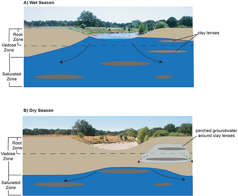
Figure 1. Conceptual model of how seasonal fluctuations in the water table and its interactions with surface water can support perched groundwater availability near intermittent rivers for GDEs in (A) Wet season and (B) Dry season.
Near-surface aquifer environments, especially at the interface of groundwater and surface water are difficult to capture in regional-scale groundwater numerical models typically used by water managers for water balancing and management. Alternatively, geophysics—specifically electrical resistivity tomography (ERT)—provides the opportunity to investigate subsurface conditions over small and large spatial scales that are applicable to understanding subsurface conditions in shallow portions of the aquifer. ERT is a well-established geophysical technique and has been used to investigate subsurface lithology (Tabbagh et al., 2000; Samouëlian et al., 2005; Sudha et al., 2009) and moisture state (Rhoades et al., 1976; Kean et al., 1987; Daily et al., 2010). Only more recently has geophysics been used to characterize and monitor the interaction between subsurface soil moisture and plant roots (Binley and Kemna, 2005; Robinson et al., 2008, 2012; Schwartz et al., 2008; Nijland et al., 2010; Ma et al., 2014; Hübner et al., 2015; Cassiani et al., 2016). ERT was more specifically used in this study to develop a subsurface conceptual model beneath each GDE.
To sustainably manage groundwater for GDEs, baselines and thresholds need to be established to prevent groundwater conditions from having impacts on ecosystem conditions. While numerous field-based studies have investigated the short- and long-term impacts of groundwater pumping on individual biological responses (i.e., growth, reproduction, recruitment, ecosystem structure, ecosystem function, and survivorship) for individual groundwater-dependent species, there are fewer studies that examine multiple biological responses across multiple groundwater-dependent species (Costanza and Mageau, 1999; Eamus et al., 2015). Integrating ecosystem-scale biological indicators into water management monitoring programs can provide water managers the ability to integrate biological concerns into basin-wide hydrological monitoring efforts. In combination with hydrological data, biological data provides an opportunity for water managers to assess the cause-and-effect relationships between the groundwater conditions and ecosystem-scale biological responses. Since it can be onerous to examine the biological response of all organisms within an ecosystem, groundwater-dependent vegetation is investigated in this study as a practical proxy for monitoring ecosystem-scale changes in GDE health. This is because changes in groundwater conditions impact not only the health of plants themselves, but also subsequently impact the food supply and habitat conditions for animals within the ecosystem. However, if a GDE is a seep or spring with little vegetation associated with it or there are particular focal groundwater-dependent species, then other proxies may be more appropriate.
This study explores the health of three groundwater-dependent riparian forests along an interconnected surface water body within groundwater basins with an unconfined aquifer, which is not bounded on top by an aquitard and the upper surface of the saturated zone is the water table. By monitoring vegetative growth, species diversity, regenerative capacity (sapling recruitment), native plant density, vegetative structure (strata), and survivorship (canopy cover remaining over time), we explore whether hydrological conditions in the subsurface are correlated with the health of GDEs. The objectives of this paper are to: (1) characterize shallow subsurface hydrological conditions in each forest using ERT, (2) identify practical biological indicators to assess the health of GDEs, and (3) evaluate how differences in hydrological conditions correlate to health indicators for groundwater-dependent riparian forests. These objectives are intended to illustrate how discipline-specific tools can be combined to solve a common problem in sustainable groundwater management. The research presented in this paper adopts this transdisciplinary approach to bridge the fields of hydrology, geophysics, and ecology to better understand how subsurface conditions can influence GDE health.
Materials and Methods
Study Site
The Cosumnes River drains ~3,400 km2 and flows 129 km westward from its headwaters at ~2,200 m in California's Sierra Nevada Mountains toward its outlet in the Sacramento-San Joaquin Delta. Within the study reach (Figure 2), the river follows the boundary between two administratively defined groundwater basins: South American Basin (Sacramento River Hydrologic Region) and Cosumnes Basin (San Joaquin River Hydrologic Region). Human reliance on groundwater for agricultural and domestic use in both basins has substantially lowered regional groundwater levels, creating two cones of depression in the groundwater basins adjacent to the Cosumnes River. Both basins are subject to California's Sustainable Groundwater Management Act of 2014 (SGMA).
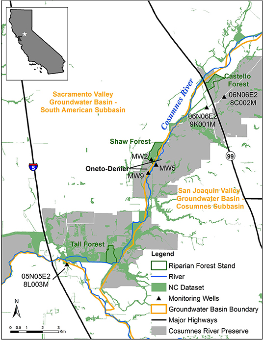
Figure 2. Study Site Map: Cosumnes River Preserve, Sacramento County, California.
A soil and geological evaluation of the study sites along the Cosumnes River was completed using USGS and CA Geological Survey maps1 and the SoilWeb interactive soil maps2 The local geology is dominated by Quaternary Period unconsolidated clays, silts, and sands deposited during the Holocene Epoch. The CA Geological Survey map shows that two deposits dominate the study area, Qha and Qhb; both are alluvial. Qha is an undivided deposit on fans, terraces, or in basins, and consists of sand, gravel, and silts that are poorly to moderately sorted. Qhb is a basin deposit consisting of fine-grained sediments from the late Holocene that were generally deposited with horizontal stratification in topographic lows. The study sites are underlain by the Columbia, Cosumnes, and San Joaquin soil units. Both the Cosumnes and San Joaquin typical pedons are silty loams and loams, compared to a typical Columbia pedon that is a fine sandy loam. All of these soil types are typical of 0–2% slopes, moderately to poorly drained, and occur along the Cosumnes River floodplain.
The Cosumnes River Preserve (Preserve) consists of over 20,000 ha of wildlife habitat that includes riparian forests, seasonal wetlands, grasslands, and habitat for birds migrating along the Pacific Flyway (Kleinschmidt Group, Inc., 2008). Three riparian stands were included in this study: Castello Forest (40 ha), Shaw Forest (60 ha), and Tall Forest (52 ha). Each of these riparian forest stands have been identified in the Natural Communities Commonly Associated with Groundwater Dataset3 (NC Dataset), which is hosted by the California Department of Water Resources (DWR). The NC dataset is a compilation of 48 publicly available State and Federal agency datasets that maps vegetation, wetlands, springs, and seeps that are commonly associated with groundwater in California (Klausmeyer et al., 2018). The overstory is dominated by valley oak (Quercus lobata) in all three forest stands, but the understory differs. The understory in Castello Forest is heavily dominated by non-native winter annual grasses, with very few shrubs or young trees. In contrast, the understory at Shaw and Tall Forests is multi-layered, containing young trees, shrubs, vines, and herbaceous plants.
Hydrologic Data
Six groundwater monitoring wells (Figure 2) were selected for this study to corroborate groundwater levels and lithological data with the ERT results. One well (MW2) is within Shaw Forest and two wells (MW5 and MW9) are within the Oneto-Denier site (open land within the Preserve). The remaining three wells are historic groundwater monitoring wells from DWR's Water Data Library4 two near Castello Forest (06N06E28C002M and 06N06E29K001M) and one near Tall Forest (05N05E28L003M). Precipitation data were accessed using the PRISM (Parameter-elevation Regressions on Independent Slopes Model) Monthly Spatial Climate Dataset5, produced by the PRISM Climate Group at Oregon State University.
Electrical Resistivity Tomography
Electrical resistivity tomography is a geophysical technique for imaging subsurface environments by transmitting electrical current from the instrument into the ground through electrodes (metal stakes inserted into the ground) along a profile. The change in the potential voltage as the current travels through the ground is measured at other adjacent electrode pairs along the profile (for more detail see Reynolds, 2011). Alternating combinations of the electrodes results in large resistivity datasets (thousands of measurements) that are collected in a relatively short time period. The resulting resistivity distributions are inverted to get the true spatial distribution of resistivity within the subsurface that describes the actual soil and moisture distributions. This results in ERT images that map how resistive the subsurface based on how quickly the electrical pulses return to the sensors at the land surface. The flow of current through the ground is controlled by the water content and soil type, and can be influenced by rapid temperature change or salinity, if present.
Seven ERT profiles were collected in total: one in Tall Forest, two in Shaw Forest, two in Castello Forest, and two at the Oneto-Denier site (Figure 3). Four ERT profiles (one in Tall, one in Shaw, and two at Castello) were collected in September 2016; and, two in Oneto-Denier and one in Shaw Forest in October 2016. ERT data was collected at the end of the summer dry season, in September 2016 and October 2016, to capture subsurface conditions when the riparian forests are most reliant on groundwater. This timing also circumvents any subsurface moisture irregularities due to rewetting fronts, because (1) no rain fell for the previous ~5 months due to the strongly seasonal Mediterranean climate, and (2) the relatively low elevation of the headwaters precluded substantial snowmelt effects on river flow. ERT data collected in September used a Multi-Phase Technologies (MPT) eight-channel resistivity system with 128 electrodes and 1-m electrode spacing. ERT data collected in October again used an MPT resistivity system, but with 112 electrodes and 1.5-m electrode spacing. The average time to collect a full dataset was ~2 h or less. A maximum current of 2,000 milliamps (mA) and 400 volts (V) was set during data acquisition, but the system automatically optimizes the injected current if less is needed; on average 42 mA and 140 V were injected during each measurement using a dipole-dipole configuration with 100% reciprocals. The ERT data were inverted using the BERT inversion code (Gunther and Rucker, 2006), which is based on a finite-element model that discretizes the subsurface as a tetrahedral mesh with a grid cell spacing equal to the electrode spacing. All ERT profiles were inverted using a flat surface, since topographic changes along each profile were <30 cm and the dense tree canopy prevented the use of a high-accuracy Global Positioning System (GPS). ERT data of low quality, defined as a measured potential <2 mV, were removed from each data set along with reciprocal errors >5%, which resulted in <10% of data removal from each data set. Model convergence resulted in a mean absolute difference (MAD) error of <6% for all ERT profiles between the measured and modeled data.
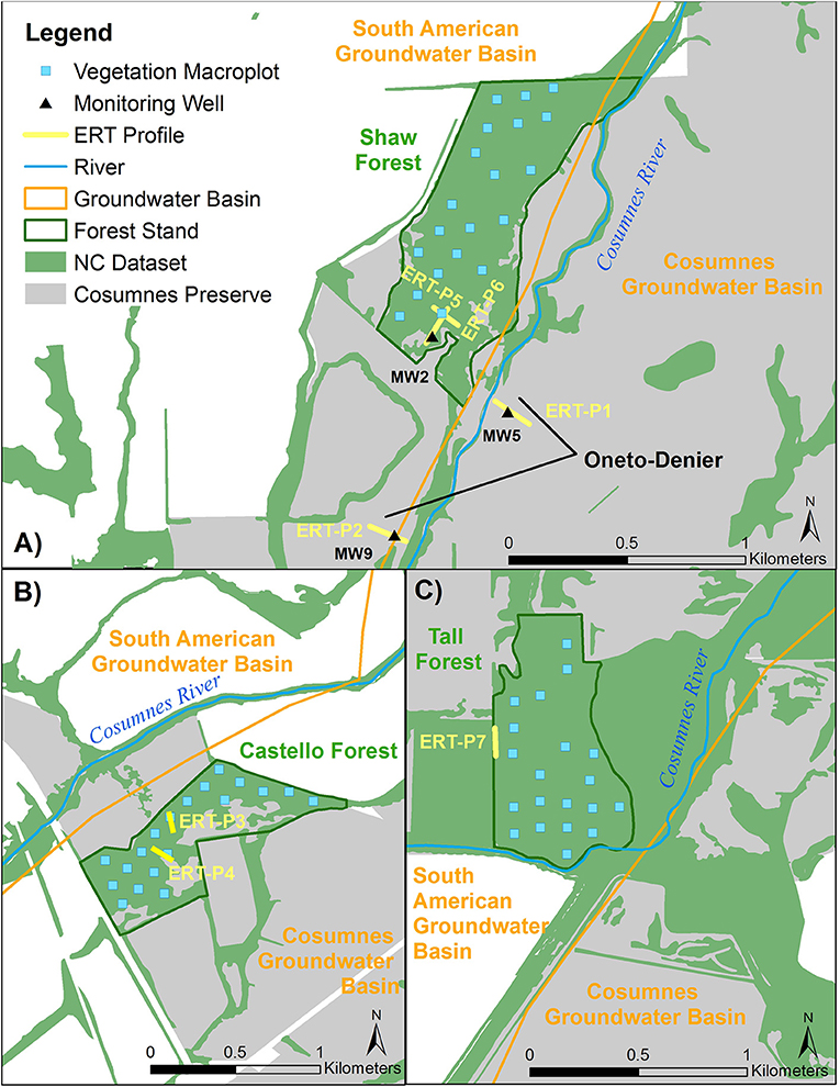
Figure 3. Location of ERT profiles, monitoring wells, and vegetation macroplots at the four study sites: (A) Shaw Forest and Oneto-Denier, (B) Castello Forest, (C) Tall Forest.
Vegetation Monitoring
Vegetation data were collected during the summer of 2016 as part of a multi-year vegetation monitoring program. Crown dieback calculations also relied on canopy cover data collected during the summer of 2013. Each forest stand was sampled with evenly spaced, permanent 20 × 20 m macroplots. We visually estimated absolute vascular plant cover by species within seven strata that were based on a simplified version of the California Wildlife Habitat Relationships protocol (CDFW, 1988) and categorized as: (1) herb, (2) small shrub (0–2 m tall), (3) tall shrub (>2 m tall), (4) tree seedling (<0.5 m tall), (5) understory tree (0.5– <10 m tall), (6) overstory tree (≥10 m tall), and (7) woody vine. For percent cover calculations, the cover class values were first converted to their midpoints (Table 1). Total canopy cover per macroplot was the mean of four spherical densiometer measurements taken at the center of the macroplot, one facing in each of the four cardinal directions (according to the manufacturer protocol; Model C, Robert E. Lemmon, Forest Densiometers). Diameter at breast height (DBH) was recorded for all mature tree individuals ≥135 cm tall (Bernhardt and Swiecki, 1991). The number of trees that were saplings (defined arbitrarily as those between 50 and 135 cm tall) and young trees (DBH of 0.1 to 10 cm) were also recorded by species.
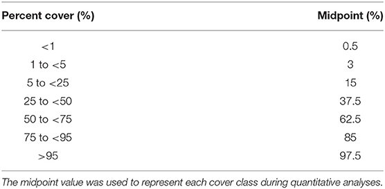
Table 1. Classes used to record the visual estimation of percent cover for each plant species as well as each stratum as a whole.
Health Indicators
Ecosystems are complex systems composed of living organisms interacting with each other and their environment (e.g., soil, water, and air). The health of an ecosystem is a measure of its overall performance resulting from the biological responses of individual species and their interaction with each other. A healthy ecosystem can be characterized as one that is sustainable—having the ability to “maintain its structure (organization) and function (vigor) over time in face of external stress (resilience)” (Costanza and Mageau, 1999). In general, stress to ecosystems caused by changes in groundwater availability can influence six key ecological processes: growth, reproduction, recruitment, mortality, ecosystem structure, and ecosystem function (Eamus et al., 2006b). In response to stress, the response functions of native plants and aquatic ecosystems follow a reasonably predictable and progressive series of events that cascade across molecular, individual, landscape, and ecosystem scales (Davies and Jackson, 2006; Eamus et al., 2006a; USEPA, 2016). For vegetation, a natural progression in response to insufficient water availability would begin with stomatal closure, resulting in a reduction in transpiration and photosynthesis. If water stress persists, xylem embolism can result in reductions in growth rates and contribute to die-back. Reduced growth would then subsequently result in a reduction in reproduction (seed set) and recruitment (sapling growth) processes that are necessary for forest succession to occur. In extreme cases of water stress, the absence of growth and recruitment of younger plants may reduce the biomass physically present in various elevations above the ground surface. The absence may also create the opportunity for new species with different growth forms (e.g., grasses instead of shrubs) to populate the area, thus changing the ecosystem structure (Eamus et al., 2006a). This could then result in the alteration of ecosystem function, since changes in ecosystem structure (the species composition and diversity) could change the functional traits expressed by individual species where the absence of key species could alter ecosystem processes, such as nutrient cycling, predator-prey relationships, and competition for resources (Chapin, 1997).
To characterize, infer, and spatially compare health conditions between forest stands in this study, six indicators were derived from the vegetation survey data: growth (species) diversity, regeneration, structure, native plant dominance, and survivorship. A brief description of the rationale and assumptions used to define each health indicator, as well as how vegetation survey data were used to quantify each indicator for this study, is provided in the subsections below.
The health indicators determined for each forest were statistically compared to the other forests in the study using the open-source software R (R Development Core Team, 2008). Mean values for each vegetation health indicator were compared between forests using a one-way ANOVA followed by the Tukey HSD statistical test. This post-hoc test was performed using the glht() function in the multcomp package (Hothorn et al., 2017). This parametric statistical test was applied using the argument vcov = vcocHC for its robustness and ability to work with unbalanced group sizes, non-normality, and heteroscedasticity (Herberich et al., 2010).
Growth
The amount of vegetative canopy cover in the overstory was used to characterize growth. Growth was quantified using a spherical densiometer, which is a handheld instrument with a spherical-shaped mirror on which small squares are engraved to assist in determining the amount of tree canopy in the mirror's reflection (Strickler, 1959). Canopy cover represents the amount of overstory tree biomass that exists at a given point in time. It is a relative value and can range from 0 to 100%, where higher percentages denote denser growth.
Diversity
The Shannon-Wiener Evenness Index, which incorporates both species richness and the abundance of each species, was used to characterize diversity. The index represents the relative abundance of different species comprising the richness of an area. The index for each forest stand was calculated using the following Shannon-Wiener Evenness Index equation:
where for each macroplot (j), H is the Shannon-Wiener Evenness Index value, S is the total number of species (richness), and pi is the proportional cover of each species (i) to the total cover of all species in the macroplot. Each index value, which varies between 0 and 1, was converted into a percentile value that ranges between 0 and 100%, where higher percentages denote greater species richness and abundance.
Regeneration
The number of saplings (defined in this study as tree individuals either 50–135 cm tall or with DBH <10 cm) present was used to characterize regeneration. The height and DBH of plants were used to reflect age, where smaller trees are younger than larger ones. At a given time, the presence of trees at different sizes, particularly smaller ones (saplings), indicates that recruitment is occurring. Regeneration was calculated using the following equation:
where for each macroplot (j), R is Regeneration, Sap is the number of saplings, YT is the number of young trees (DBH 10–25 cm), and MT is the number of mature trees (DBH >25 cm). Regeneration was converted into a percentile value that ranges between 0 and 100%, where higher percentages denote greater recruitment.
Structure
Ecosystem structure is generally defined as the community of living organisms coexisting in conjunction with abiotic components (e.g., soil, air, and water). In most habitats, vegetation provides the main structure of the environment (Rutten et al., 2015). More vertical structure (or vertical layering) creates habitat complexity that can support a greater vertical distribution of birds (Pearson, 1971), mammals (Grelle, 2003), and insects (Schulze et al., 2001). Vertical stratification, or the number of layers (strata) present, was used to characterize ecosystem structure and was calculated using the following equation:
where for each macroplot (j), ES is the ecosystem structure, Strata is the number of strata, and Stratamax is the maximum number of strata. In this case, Stratamax was seven based on the chosen protocol to characterize vegetation. Ecosystem structure was converted into a percentile value that ranges between 0 and 100%, where higher percentages denote greater vertical structure in the forest.
Native Plant Dominance
Native plant dominance was used as a health indicator because it can provide insight on whether the ecosystem's function is intact. Ecosystem function is generally defined as an ecosystem's ability to maintain multiple functions, such as carbon storage, nutrient cycling, and the transfer of energy via growth and decomposition. Functional responses to stress induced by changes in groundwater have been reported to cause changes in community composition such that native species are outcompeted by non-native species (Keddy and Reznicek, 1986; Moore and Keddy, 1988; Sommer and Froend, 2014). Numerous studies have also shown the ability of non-native invasive species to alter the flow of energy and cycling of materials within an ecosystem, and thus its functioning (Vitousek et al., 1987; D'Antonio, 1992; Vitousek, 1997; Gordon, 1998; Mack and D'Antonio, 1998; Cicchetti and Diaz, 2002; Meyerson et al., 2002; Ehrenfeld, 2003; Kourtev et al., 2003; Levine et al., 2003; Dukes and Mooney, 2004; USEPA, 2016). Although the presence of non-native invasive species may not necessarily alter the functioning of an ecosystem (Barney et al., 2013), the presence of native species can at a minimum be indicative that ecosystem function is more likely to be intact. In this study, we use native plant dominance as a rough proxy for ecosystem function, which was calculated by comparing the percent of native plant cover to total plant cover:
where for macroplot (j), F is the ecosystem function, NP is the total cover of native plant species, and IP is the total cover of introduced (non-native) plant species. Ecosystem function was converted into a percentile value that ranges between 0 and 100%, where higher values denote greater function.
Survivorship
The percentage of overstory vegetation cover remaining from 2013 to 2016 was used to characterize survivorship and was quantified using spherical densiometer data. Survivorship was calculated using the following equation:
where for macroplot (j), S is survivorship, SD is the spherical densiometer value, (t) represents data from 2016, and (t-1) represents data from 2013. Survivorship was converted into a percentile value, where higher percentages denote less crown dieback. Percentages over 100% were possible if cover increased during this time period.
Results
Hydrologic Conditions
Figure 4 shows precipitation by month and groundwater levels for three wells from the mid-1960s through August 2019. Historical depth to groundwater (defined as the position of the water table relative to the ground surface) near Castello Forest has ranged between 9.0 and 25.2 m at 06N06E28C002M (Figure 4B) and 5.1 and 23.7 m at 06N06E29K001M (Figure 4C), and near Tall forest has ranged between 0.5 and 3.7 m at 05N05E28L003M (Figure 4D). Depth to groundwater in the unconfined aquifer at four of the ERT sites (ERT-P1, ERT-P2, ERT-P5, and ERT-P6) fluctuated between 6.2 and 14.0 m at MW5, 1.5 and 12.0 m at MW9, and 4.2 and 13.1 m at MW2 (Figure 5), since groundwater data collection began in December 2012. At all three monitoring wells within the study area, depth to groundwater was deepest after the dry summer season and before the rainy winter season. Depth to groundwater gradually increased between 2012 and 2016, which corresponds to the historic drought conditions California experienced during this period. At the time of ERT data collection, depth to groundwater was 11.6 m at ERT-P1, 10.0 m at ERT-P2, and 12.5 m at ERT-P6.
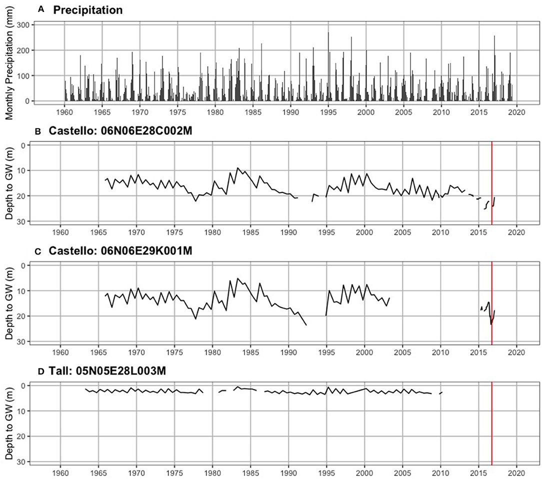
Figure 4. Long-term hydrologic time series. (A) Monthly precipitation (mm), and depth to groundwater in the unconfined aquifer (meters below ground surface) near (B) Castello forest, (C) Castello forest, and (D) Tall forest. The vertical red line denotes when ERT data collection occurred nearby.
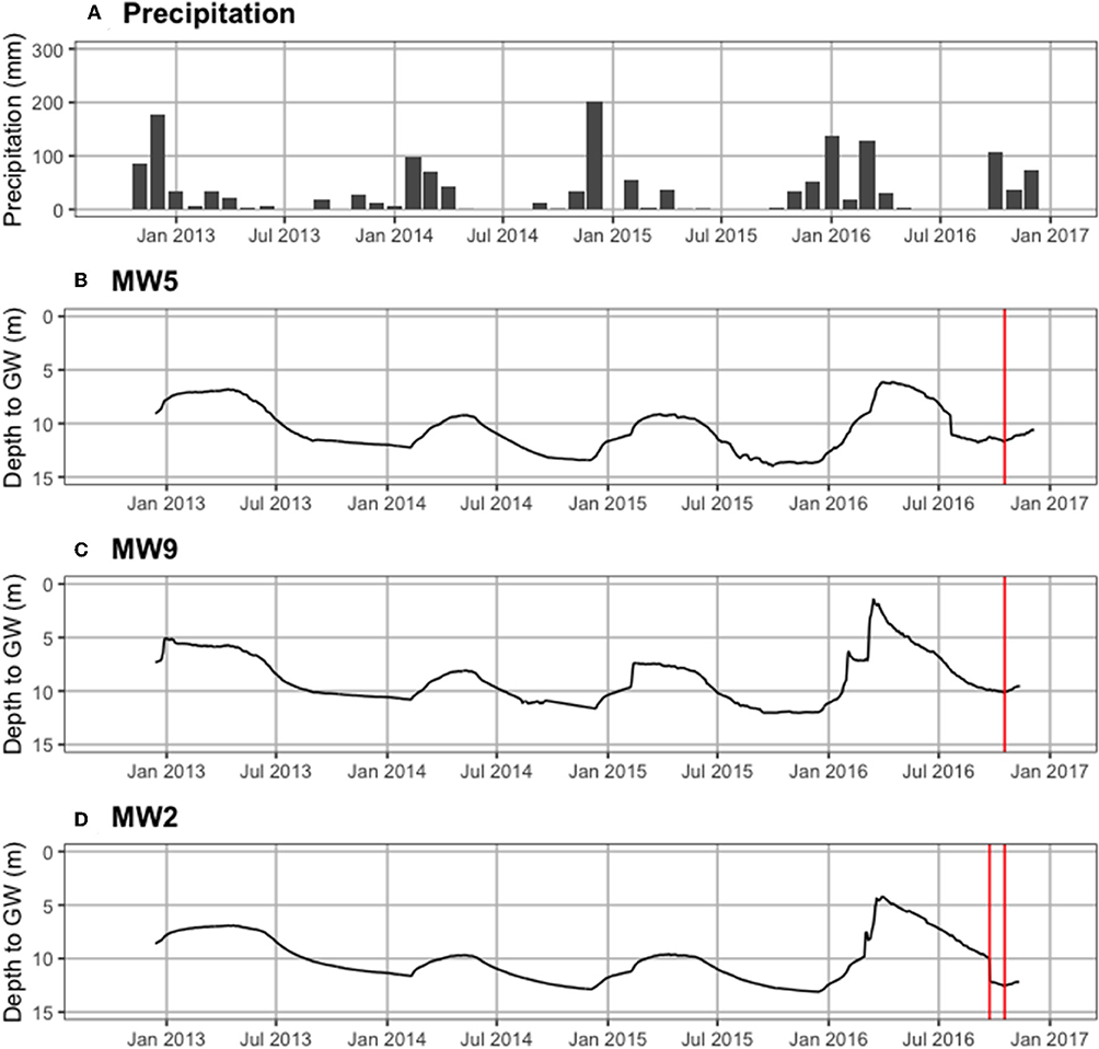
Figure 5. Recent hydrologic time series. (A) Monthly precipitation (mm), and depth to groundwater in the unconfined aquifer (meters below ground surface) at (B) MW5 in Oneto-Denier, (C) MW9 in Oneto-Denier, and (D) MW2 in Shaw forest. The vertical red line denotes when ERT data collection occurred at each site.
Electrical Resistivity Tomography
The following subsections outline the ERT results from the Oneto-Denier area and each forest block (Castello, Shaw, and Tall). At the time of the survey no rainfall had been recorded in the area for 5+ months, leaving the water table at the bottom extents of the ERT images. Data acquisition was completed in <2 h per profile and temperatures remained constant throughout the survey. The study area is known to have low salinity. Therefore, ERT responses are interpreted as a function of soil texture and water content. Well logs indicate the lower resistivity values (20 Ωm or less) to be associated with clay-dominated sediments, and higher resistivity values (40 Ωm and greater) with sand-dominated sediments.
Oneto-Denier
ERT-P1 results (Figure 6) show some lateral and vertical soil heterogeneity. The MW5 lithologic log (Figure 6B) is dominated by silts and clays with some sand that result in low (cool colors) resistivity values throughout the profile, with the exception of a slightly more resistive zone at 6–12 m depth from 60 to 120 m along the profile, which we interpret is associated with sandier material below the more laterally extensive silt and clay observed in the lithologic log. Near the river bank at the beginning of ERT-P1 (0–50 m along the profile) we observed a shallow highresistivity zone that corresponds to coarser alluvial substrate that has been deposited in an eroded elevated part of the channel (like an over-flow channel) when stream flows exceed capacity. The deposition of these coarse sediments is expected to be the cause of this shallow high-resistive zone. The ERT results correlated well with local geologic maps1 and lithologic data from the MW5 well log (Figure 6B). At the time of ERT-P1 data acquisition, the groundwater table (pink triangle, Figure 6B) at MW5 was 11.6 m below ground and was obscured by the clay content of the local soil.
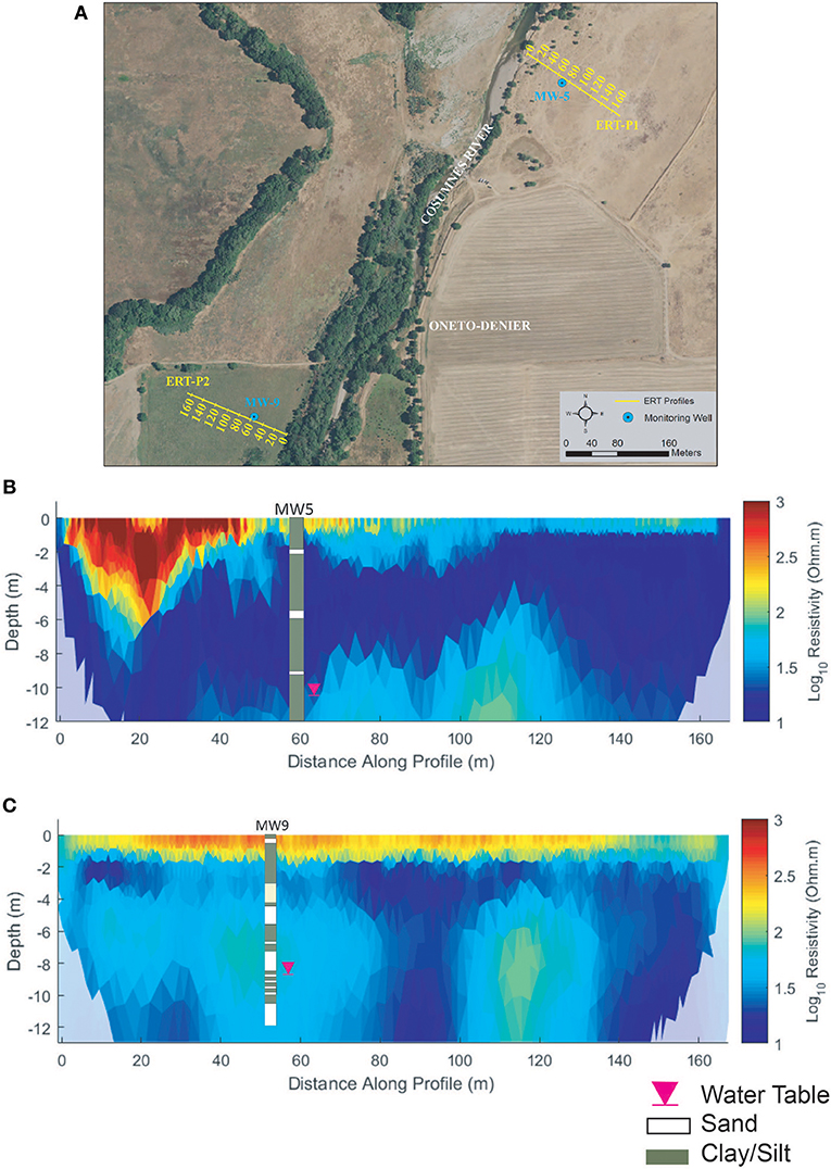
Figure 6. Oneto-Denier (A) ERT study site, (B) ERT-P1 inversion results, and (C) ERT-P2 inversion results. ERT data were collected in October 2016 after significant rainfall (~5 cm). The water table at the time of data collection is denoted by the pink inverted triangle.
The results for ERT-P2 (Figure 6C) show strong heterogeneity both laterally and vertically, where more resistive soils at 40–60 m (depth of 6–10 m) and 100–130 m (depth of 6–12 m) indicate sandy soil zones that are consistent with the MW9 lithological log data. At the time of ERT-P2 data acquisition, the groundwater table at MW9 was 10.0 m below ground (pink triangle, Figure 6C) and again was obscured by the soil texture.
Both ERT-P1 and ERT-P2 exhibit a more resistive layer near the ground surface (<2 m depth), which likely corresponds to and is affected by the vegetative root zone. Differences in the duration of plant water uptake between ERT-P1 (dead winter annual grass) and ERT-P2 (live perennial grass) likely contributed to the more resistive topsoil in ERT-P2.
Overall, results from ERT-P2 and lithologic logs indicate the west side of the river at Oneto-Denier has slightly more sandy soils than ERT-P1 on the east side of the river. The observed differences in soil type at depth between ERT-P1 and ERT-P2 are supported by the geologic and land history record. The geologic map (how to cite?) shows the very clay-dominated Riverbank Formation underlying soils on the east side of the river at this latitude. Recent compilation and interpretation of historical documents indicates that in the mid-1800s, the Cosumnes River ran west of its current course, breaking into distributaries just south of present-day Shaw Forest and creating a mosaic of seasonal and perennial wetlands (Whipple et al., 2012).
Castello Forest
Profiles ERT-P3 and ERT-P4 were collected at Castello Forest (Figure 7A) adjacent to macroplots (MP) MP-6 and MP-13, respectively. ERT-P3 was enclosed within the canopy of mature trees except for a gap at ~70 m, and ERT-P4 was positioned across a boundary between mature canopy and a more open area dominated by annual grasses with few scattered shrubs. Both ERT-P3 and ERT-P4 (Figures 7B,C) show a more resistive subsurface with greater vertical heterogeneity than any of the other ERT profiles (see Figures 6B,C, 8B,C, 9B,C). In ERT-P3, a zone of higher resistivity in the near surface (~2 m depth) extends along the entire profile except where it thins to ~1 m depth around 70 m (red box, Figure 7B). This variation in the near-surface resistive zone is consistent with the greater water demands and water lifting capabilities of mature trees as compared to shallowly rooted grasses. Likewise, from 0 to 40 m in ERT-P4, the near-surface resistive zone is thinner than after the transition from the grass to the tree coverage (red box, Figure 7C), again showing a potential influence of plant life form (grass vs. tree) on soil moisture. Beyond 40 m in ERT-P4 within the tree coverage, the near-surface resistive zone extends even slightly deeper than observed in ERT-P3. Given the overall higher subsurface resistivity values at Castello Forest, along with the observed sandier surface soils and their similarity to the higher resistivity values in the sandy soil zones in ERT-P2 (MW9), these soils are interpreted as sandy.
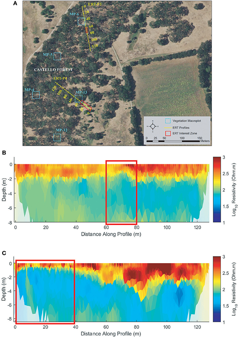
Figure 7. Castello Forest (A) ERT study site, (B) ERT inversion results for ERT-P3, and (C) ERT inversion results for ERT-P4. Red boxes denote sections along the ERT transect with less woody vegetation and resulting wetter soils (low resistivity) compared to remainder of the vegetated transect line.
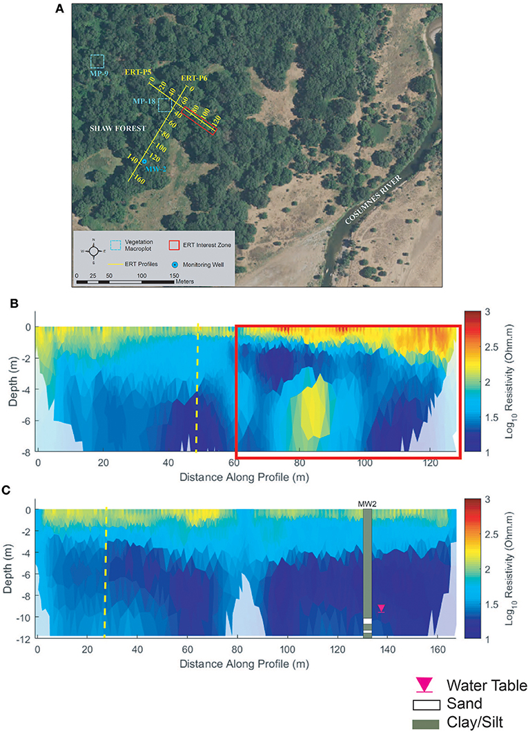
Figure 8. Shaw forest (A) ERT study site, (B) ERT inversion results for ERT-P5, and (C) ERT inversion results for ERT-P6. Dashed yellow lines in (B,C) denote the intersection point between these two ERT profiles. The red box in (B) denotes the section of the ERT profile that is more vegetated by thick blackberry bushes, resulting in higher resistivity.
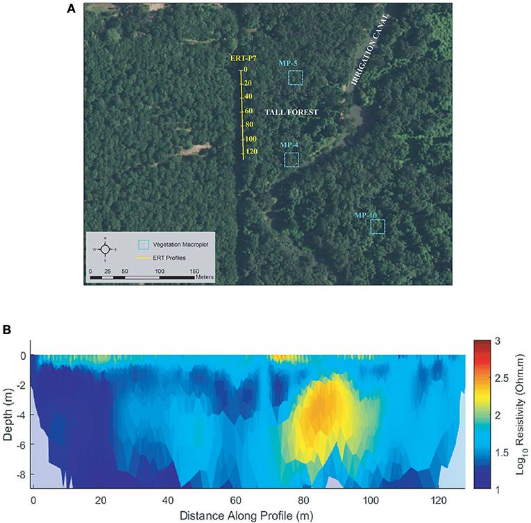
Figure 9. Tall Forest (A) ERT study site and (B) ERT inversion results for ERT-P7.
Shaw Forest
Perpendicular profiles ERT-P5 and ERT-P6 were collected at Shaw Forest (Figure 8A) adjacent to MP-18 and MW-2, respectively. ERT-P5 results (Figure 8B) indicate silt/clay soils, much like those at ERT-P1 (Oneto-Denier), with both vertical and lateral soil heterogeneity. Nearby lithologic data from the MW-2 well log indicate pervasive silts and clays from 0 to 12 m depth. Resistivity values along ERT-P5 show agreement with this well log, except at 80 m where there is an isolated zone of low resistivity that is interpreted as sandier soils (based on interpreted resistivity values at ERT-P2, ERT-P3, and ERT-P4). The near-surface soils (<2 m depth) are more resistive from 60 to 128 m along ERT-P5, which correlates to denser understory vegetation (red box, Figure 8B). A lower density of understory vegetation along the first half of ERT-P5 correlates with less resistive near-surface soils. The ERT-P6 profile correlates well with MW2 (Figure 8C) and the low-density understory vegetation matches with less resistive near-surface soils (<2 m depth). The vegetation along ERT-P6 and the beginning (0–60 m) of ERT-P5 comprised the same dominant plant species compared to the end of ERT-P5.
Tall Forest
One ERT profile (ERT-P7) was collected at Tall Forest (Figure 9) adjacent to a dirt access road just inside the edge of the forest due to the density of the forest undergrowth. ERT-P7 resistivity results (Figure 9B) show low resistivity conditions with mild lateral and vertical heterogeneity. Although there are no monitoring wells nor lithological logs in Tall Forest, ERT-P7 resistivity values were compared to the range of values in Shaw Forest and Oneto-Denier, where monitoring wells exist. The subsurface soils at ERT-P7 are interpreted as silt and clay deposits from 0 to 60 m along the profile. Conversely, beyond 60 m the soils show slightly higher resistivity, which based on results observed at ERT-P2 were interpreted as slightly sandier.
Vegetation Health Indicators
For each forest stand, summary statistics were calculated for: (1) the 2013 and 2016 vegetation survey data (Table 2) used to calculate each health indicator, and (2) the six health indicators for each forest (Table 3; Figure 10). Castello Forest was found to be statistically different (p < 0.05) from both Shaw Forest and Tall Forest for all six health indicators. Shaw Forest and Tall Forest were statistically similar (Table 3) for four of the health indicators (growth, diversity, structure, and survivorship), and statistically different (p < 0.05) for two of the health indicators (regeneration and native plant dominance). Castello Forest scored lower than both Shaw Forest and Tall Forest on every health indicator, and Tall Forest scored higher than Shaw Forest for the regeneration and native plant dominance indicators. Relative differences in health indicators between forests resulted in Castello Forest having the least healthy conditions due to lower growth, species diversity, regeneration, vertical structure, and survivorship of canopy from between 2013 and 2016. Health conditions of Tall and Shaw Forests were more similar to each other in comparison to Castello Forest, but slightly higher scores for regeneration and native plant dominance resulted in Tall Forest having the healthiest conditions.
Table 2. Summary statistics for vegetation data included in analyses.
Table 3. Statistical results for each ecological health indicator.
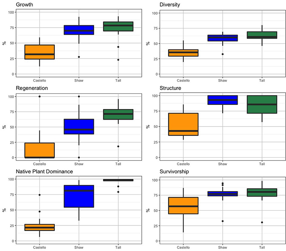
Figure 10. Box plots for each vegetation health indicator by forest stand. Dots represent data points outside the 25th and 75th percentiles (represented as the vertical, thin black line).
Discussion
Lithological and Hydrological Conditions
Subsurface lithological conditions in each forest were characterized using ERT and lithological logs from available monitoring wells. These independent data sources corroborated each other and indicated broad qualitative differences across the forest stands studied. Castello Forest showed sandier soils than Shaw and Tall Forests, which both showed high clay/silt content.
Strong precedence exists to link soil texture as imaged by ERT with the hydrological factor of soil moisture. It is broadly accepted that clays and silts have much greater water retention capacity than sands. Development of the ERT method identified soil moisture as a separate factor influencing resistivity, and when present with clay, the two are highly correlated. These principles developed from empirical testing were applied in a similar study by Robinson et al. (2008), where soil electrical conductivity (inverse of resistivity) was used to map soil spatial distributions across a large landscape with diverse plant communities. After testing soil samples for clay content and volumetric water content, they found soil resistivity to be controlled by both factors, which were also positively correlated with each other and soil water retention. These results are very similar to findings from this study, where low resistivity values were associated with soils of high clay content as observed in well logs. We therefore adopt the fundamental concept that water retention was higher in our clay-rich soils compared to the sandier soils.
Hydrologic evidence from the lower Cosumnes study system also strongly supports the connection between ERT measurements and soil moisture. Figures 4, 5 show that the predominance of silt and clay that was observed in Tall Forest was also coincident with the shallowest groundwater levels observed through the historical record over nearly 50 years (Figure 4C), with groundwater levels ranging between 0.5 and 3.7 m. In contrast, Castello forest had predominantly sandy soils and the deepest groundwater levels observed (5.1–25.2 m; Figures 4A,B). Four years of data over a prolonged drought show that Shaw Forest had groundwater levels intermediate between these two (4.2–13.5 m; Figure 5C). Therefore, groundwater availability (higher soil moisture content and shallower groundwater levels) increased progressively downstream from Castello Forest to Shaw Forest to Tall Forest. Increasing groundwater availability along the Cosumnes River is likely a combination of groundwater flow gradients and soil type differences between forests. The spatial distribution of riparian forests along this groundwater gradient provides an opportunity to observe which groundwater levels are supportive of healthy conditions within a GDE.
GDE Health
In this study, we developed an approach to quantify ecosystem health within GDEs, using metrics of groundwater-dependent vegetation as indicators, so that health conditions could be statistically compared across the landscape. Vegetation indicators used to infer GDE health conditions demonstrated that Shaw and Tall Forests have statistically similar and greater health conditions than Castello Forest. One of the major biological differences between the forests was that Shaw and Tall Forests both had a lush understory, whereas Castello Forest did not. This difference was captured in the vegetative growth, regeneration, and structure indicators, such that both Shaw and Tall Forests exhibited higher vegetative growth (canopy cover), regeneration (sapling recruitment), and structure (number of strata present, including young trees) than Castello Forest. A lack of regeneration at Castello Forest indicates that health conditions may be in an unsustainable state in comparison to Shaw and Tall Forests.
Greater vertical structure at Tall and Shaw Forests compared to Castello Forest was also correlated to the diversity and native plant dominance indicators. Greater species diversity in Tall and Shaw Forests in comparison to Castello Forest was also accompanied by a greater proportion of native plant cover. These observations are consistent with previous research studies, which found changes in groundwater availability to cause a functional shift in the ecosystem away from native habitat toward more favorable conditions for invasive species (Keddy and Reznicek, 1986; Moore and Keddy, 1988; Sommer and Froend, 2014).
Hydrological Controls on GDE Health
On the larger scale of the river reach studied, comparisons among ERT profiles and groundwater monitoring well data showed that clay-dominated sites (Shaw and Tall Forests) had shallower depth to groundwater, retained more soil moisture, and sustained healthier vegetation than the sandier site (Castello Forest), with its greater depth to groundwater, reduced soil moisture, and less healthy vegetation. This shows the strong influence of groundwater availability and soil type on groundwater-dependent riparian vegetation. Further studies may elucidate more detailed mechanisms shaping groundwater availability, such as hydraulic effects of root networks and surface flood regimes. Further work may also refine the spatial scale at which within-forest differences could be affected by small-scale variations in underlying sediments. Our study, however, operated at the scale of entire forest stands underlain by a sequence of substantially different groundwater and soil conditions that together influenced subsurface water retention and availability of that water to a broad suite of plant species.
Therefore, differences in groundwater availability are most likely the cause for the observed differences in ecosystem health at our study sites, due to the spatial differences in groundwater availability influenced by soil type and the groundwater level gradient along the Cosumnes River. Our results support our hypothesis that differences in ecosystem health correlate to hydrological conditions, such that access to greater subsurface moisture from shallower groundwater levels results in the healthier conditions that were observed in Shaw and Tall Forests in comparison to Castello Forest.
Some groundwater-dependent plants may have the adaptive capacity to cope with absolute and relative changes to groundwater availability depending on the rate, magnitude, and duration of groundwater changes. However, previous research demonstrates that if absolute and relative groundwater changes are too drastic for rooting networks to adapt, groundwater changes can result in a spectrum of biological responses, which can range in severity from declines in productivity to increased mortality (Scott et al., 1999; Shafroth et al., 2000; Canham et al., 2012, 2015). Even in cases where some individual groundwater-dependent plants have the capacity to adapt to gradual increases in water stress due to groundwater decline, changes in the ecosystem structure and community composition can still result (Froend and Sommer, 2010). This phenomenon is consistent with the decrease in number of strata and greater presence of non-native species in Castello Forest in contrast to Shaw and Tall Forests, thereby suggesting that long-term trends in groundwater conditions may be contributing to the poorer health conditions observed in Castello Forest.
The absence of understory trees at Castello Forest sends a strong biological signal that regeneration is lacking and that the current groundwater regime may not be accessible to younger plants with shallower root systems. This is problematic because if the groundwater regime is not restored to conditions where sapling recruitment can occur, there will be no younger trees present to replace mature trees once they inevitably reach mortality. Groundwater depths near Castello Forest were also deeper than the water depth value of ~10 m that is often used to indicate the likelihood that plant rooting depths are capable of accessing groundwater (Canadell et al., 1996; Eamus et al., 2015; Rohde et al., 2018). Routine monitoring of health indicators within each of the forest blocks, in conjunction with groundwater level data from monitoring wells over time, would help identify the groundwater level thresholds necessary to enable regeneration and support GDE health in this area. However, healthy conditions in Shaw Forest provide a preliminary insight into what groundwater levels (observed at MW2) may be necessary to support nearby riparian forests. With only 5 years of groundwater level data available at MW2, continuous monitoring of groundwater levels and biological responses over time would help elucidate cause-and-effect relationships between groundwater and the riparian forest, so adaptive management can occur as more information becomes available.
Conclusion
This transdisciplinary study exemplifies the utility of combining geophysical, geological, hydrological, and biological data to explore potential groundwater impacts on GDEs in an unconfined aquifer system. Hydrologic data gaps in interconnected surface water systems are common due to heterogeneous subsurface conditions, but are important to understand since the interconnections between surface water and groundwater can support perched groundwater, which can offer an accessible source of groundwater to riparian vegetation when unconfined aquifers are too deep. While it may be difficult to accurately represent subsurface conditions in these aquifer settings using sparse monitoring well networks and numerical groundwater models, geophysics offers a complementary approach for deducing the subsurface structure and soil moisture distribution within ecosystems. Transdisciplinary approaches such as these can elucidate insights on how these systems functionally respond to changes or spatial differences in groundwater availability.
This study also demonstrated the value of using vegetation survey data to deduce GDE health. Vegetation survey data offers the ability to determine a wide variety of biological responses in an ecosystem ranging from growth to survivorship, which can be used to investigate groundwater impacts to ecosystems. It is highly advised that groundwater sustainability managers interpret biological information in conjunction with hydrologic data so that only those changes to ecosystem health due to groundwater are addressed (Rohde et al., 2018). It is important to note that although using vegetation data to deduce ecosystem health is best used as a surveillance indicator in routine monitoring, that it may overlook some critical biological responses of rare, threatened, and endangered species. In these circumstances, it is highly advised that water managers consider additional biological investigations that can better characterize the condition of these valuable environmental assets.
Successful implementation of sustainable groundwater legislation relies on practical biological and hydrologic metrics that can be incorporated into monitoring regimes. For practical reasons, monitoring regimes should at a minimum provide some basic surveillance of the hydrologic conditions supporting GDEs and the biological conditions within the GDE, so that cause-and-effect relationships can be deduced. Practical biological indicators that can integrate ecosystem-scale biological data into water management monitoring programs and be used to assess the health of GDEs in relation to hydrological conditions are necessary but often missing in groundwater management and monitoring programs. This study provides an approach for water managers to integrate practical biological indicators that can characterize GDE health into monitoring programs, so that groundwater thresholds can be locally determined and adverse impacts to ecosystems can be avoided. By monitoring GDE health over time, water practitioners can determine if a correlation exists between GDE health metrics and hydrologic datasets that signal that potential groundwater impacts to the ecosystem are occurring. This would help water managers identify groundwater thresholds that can sustain GDEs and prioritize limited funds and management efforts so that adaptive management of GDEs under sustainable groundwater management can ensue.
Author Contributions
MR was the lead researcher, developed the ecosystem health indicators, analyzed the results, and drafted the manuscript. SS led collection and management of the vegetation survey data, assisted with the ERT data collection, helped in all aspects of the research especially those pertaining to the vegetation data, and assisted with the writing of the manuscript. CU collected and analyzed all of the ERT data, and assisted in writing of the manuscript. JH assisted in the analysis and writing.
Funding
We would like to thank the S. D. Bechtel, Jr. Foundation for their philanthropic financial support to The Nature Conservancy's ongoing groundwater research on GDEs in sustainable groundwater management.
Conflict of Interest
The authors declare that the research was conducted in the absence of any commercial or financial relationships that could be construed as a potential conflict of interest.
Acknowledgments
The authors would like to thank The Nature Conservancy's seasonal staff (Audrey Kelly, Victor Oelschlaegel, Troy Shea, and Jane Thompson) for their help in the field with vegetation monitoring and geophysical data collection. We also would like to thank Jesse Roseman for inspiring this research work in the Cosumnes River Preserve. We also thank Dr. Graham Fogg, Stephen Maples, and Alysa (Amy) Yoder at the University of California, Davis for providing monitoring well data within the Cosumnes River Preserve. We also thank Dr. Baptiste Dafflon and Dr. Emmanuel Leger for their help interpreting ERT data by integrating the BERT inversion code using Matlab routines.
Footnotes
1. ^ftp://ftp.consrv.ca.gov/pub/dmg/rgmp/Prelim_geo_pdf/Lodi_100K_prelim.pdf
2. ^https://casoilresource.lawr.ucdavis.edu/soilweb-apps/
3. ^https://gis.water.ca.gov/app/NCDatasetViewer/
4. ^http://wdl.water.ca.gov/waterdatalibrary/
5. ^https://developers.google.com/earth-engine/datasets/catalog/OREGONSTATE_PRISM_AN81m
References
Barney, J. N., Tekiela, D. R., Dollete, E. S., and Tomasek, B. J. (2013). What is the “real” impact of invasive plant species? Front. Ecol. Environ. 11, 322–329. doi: 10.1890/120120
Bernhardt, E. A., and Swiecki, T. J. (1991). Guidelines for Developing and Evaluating Tree Ordinances. Available online at: http://www.isa-arbor.com/education/resources/educ_treeordinanceguidelines.pdf (accessed March 16, 2017).
Binley, A., and Kemna, A. (2005). “DC resistivity and induced polarization methods,” in Hydrogeophysics, eds Y. Rubin and S. S. Hubbard (Dordrecht: Springer, 129–156.
Blevins, E., and Aldous, A. (2011). Biodiversity Value of Groundwater-Dependent Ecosystems. Portland, OR: Wetland Science & Practice, 18–24. Available online at: https://www.conservationgateway.org/ConservationByGeography/NorthAmerica/UnitedStates/oregon/freshwater/Documents/GW_Blevins%20and%20Aldous_2011_WSP.pdf (accessed October 28, 2019).
Canadell, J., Jackson, R. B., Ehleringer, J. B., Mooney, H. A., Sala, O. E., and Schulze, E. D. (1996). Maximum rooting depth of vegetation types at the global scale. Oecologia 108, 583–595. doi: 10.1007/BF00329030
Canham, C. A., Froend, R. H., and Stock, W. D. (2015). Rapid root elongation by phreatophyte seedlings does not imply tolerance of water table decline. Trees 29, 815–824. doi: 10.1007/s00468-015-1161-z
Canham, C. A., Froend, R. H., Stock, W. D., and Davies, M. (2012). Dynamics of phreatophyte root growth relative to a seasonally fluctuating water table in a mediterranean-type environment. Oecologia 170, 909–916. doi: 10.1007/s00442-012-2381-1
Cassiani, G., Boaga, J., Rossi, M., Putti, M., Fadda, G., Majone, B., et al. (2016). Soil–plant interaction monitoring: small scale example of an apple orchard in Trentino, North-Eastern Italy. Sci. Total Environ. 543, 851–861. doi: 10.1016/j.scitotenv.2015.03.113
CDFW (1988). A Guide to Wildlife Habitats of California. Available online at: https://www.wildlife.ca.gov/Data/CWHR/Wildlife-Habitats (accessed December 12, 2018).
Chapin, F. S. III. (1997). Biotic control over the functioning of ecosystems. Science 277, 500–504. doi: 10.1126/science.277.5325.500
Cicchetti, G., and Diaz, R. J. (2002). “Types of salt marsh edge and export of trophic energy from marshes to deeper habitats,” in Concepts and Controversies in Tidal Marsh Ecology, eds M. P. Weinstein and D. A. Kreeger (Dordrecht: Kluwer Academic Publishers), 515–541.
Costanza, R., and Mageau, M. (1999). What is a healthy ecosystem? Aquatic Ecol. 33, 105–115. doi: 10.1023/A:1009930313242
Daily, W., Ramirez, A., LaBrecque, D., and Nitao, J. (2010). Electrical resistivity tomography of vadose water movement. Water Resour. Res. 28, 1429–1442. doi: 10.1029/91WR03087
D'Antonio, C. (1992). Biological invasions by exotic grasses, the grass fire cycle, and global change. Annu. Rev. Ecol. Syst. 23, 63–87. doi: 10.1146/annurev.es.23.110192.000431
Davies, S. P., and Jackson, S. K. (2006). The biological condition gradient: a descriptive model for interpreting change in aquatic ecosystems. Ecol. Appl. 16, 1–16. doi: 10.1890/1051-0761(2006)016[1251:TBCGAD]2.0.CO;2
Dukes, J. S., and Mooney, H. A. (2004). Disruption of ecosystem processes in western North America by invasive species. Rev. Chil. Hist. Nat. 77, 411–437. doi: 10.4067/S0716-078X2004000300003
Eamus, D., Froend, R., Loomes, R., Hose, G., and Murray, B. (2006a). A functional methodology for determining the groundwater regime needed to maintain the health of groundwater-dependent vegetation. Aust. J. Bot. 54:97. doi: 10.1071/BT05031
Eamus, D., Hatton, T., Cook, P., and Colvin, C. (2006b). Ecohydrology: Vegetation Function, Water and Resource Management. Collingwood, VIC: CSIRO Publishing.
Eamus, D., Zolfaghar, S., Villalobos-Vega, R., Cleverly, J., and Huete, A. (2015). Groundwater-dependent ecosystems: recent insights from satellite and field-based studies. Hydrol. Earth Syst. Sci. 19, 4229–4256. doi: 10.5194/hess-19-4229-2015
Ehrenfeld, J. G. (2003). Effects of exotic plant invasions on soil nutrient cycling processes. Ecosystems 6, 503–523. doi: 10.1007/s10021-002-0151-3
Fleckenstein, J. H., Niswonger, R. G., and Fogg, G. E. (2006). River-aquifer interactions, geologic heterogeneity, and low-flow management. Ground Water 44, 837–852. doi: 10.1111/j.1745-6584.2006.00190.x
Froend, R., and Sommer, B. (2010). Phreatophytic vegetation response to climatic and abstraction-induced groundwater drawdown: examples of long-term spatial and temporal variability in community response. Ecol. Eng. 36, 1191–1200. doi: 10.1016/j.ecoleng.2009.11.029
Gleeson, T., Befus, K. M., Jasechko, S., Luijendijk, E., and Cardenas, M. B. (2015). The global volume and distribution of modern groundwater. Nat. Geosci. 9, 161–167. doi: 10.1038/ngeo2590
Gordon, D. R. (1998). Effects of invasive, non-indigenous plant species on ecosystem processes: lessons from Florida. Ecol. Appl. 8, 975–989. doi: 10.1890/1051-0761(1998)008[0975:EOINIP]2.0.CO;2
Grelle, C. E. V. (2003). Forest structure and vertical stratification of small mammals in a secondary atlantic forest, Southeastern Brazil. Stud. Neotrop. Fauna Environ. 38, 81–85. doi: 10.1076/snfe.38.2.81.15926
Gunther, T., and Rucker, C. (2006). “A new joint inversion approach applied to the combined tomography of DC resistivity and seismic refraction data,” in Society of Exploration Geophysicists, 1196–1202.
Herberich, E., Sikorski, J., and Hothorn, T. (2010). A robust procedure for comparing multiple means under heteroscedasticity in unbalanced designs. PLoS ONE 5:e9788. doi: 10.1371/journal.pone.0009788
Hothorn, T., Bretz, F., Westfall, P., Heiberger, R. M., Schuetzenmeister, A., and Scheibe, S. (2017). multcomp: Simultatenous Interference in General Parametric Models. Available online at: https://cran.r-project.org/web/packages/multcomp/multcomp.pdf (accessed July 12, 2018).
Hübner, R., Heller, K., Günther, T., and Kleber, A. (2015). Monitoring hillslope moisture dynamics with surface ERT for enhancing spatial significance of hydrometric point measurements. Hydrol. Earth Syst. Sci. 19, 225–240. doi: 10.5194/hess-19-225-2015
Kean, W. F., Waller, M. J., and Layson, H. R. (1987). Monitoring moisture migration in the vadose zone with resistivity. Ground Water 25, 562–571. doi: 10.1111/j.1745-6584.1987.tb02886.x
Keddy, P. A., and Reznicek, A. A. (1986). Great lakes vegetation dynamics: the role of fluctuating water levels and buried seeds. J. Great Lakes Res. 12, 25–36. doi: 10.1016/S0380-1330(86)71697-3
Klausmeyer, K. R., Howard, J. K., Keeler-Wolf, T., Davis-Fadtke, K., Hull, R., and Lyons, A. (2018). Mapping Indicators of Groundwater Dependent Ecosystems in California: Methods Report. San Francisco, CA: The Nature Conservancy.
Kleinschmidt Group, Inc. (2008). Cosumnes River Preserve Management Plan. Sacramento, CA: Privately Published. Available online at: http://cosumnes.org/documents/managementplan.pdf (accessed October 28, 2019).
Kourtev, P. S., Ehrenfeld, J. G., and Häggblom, M. (2003). Experimental analysis of the effect of exotic and native plant species on the structure and function of soil microbial communities. Soil Biol. Biochem. 35, 895–905. doi: 10.1016/S0038-0717(03)00120-2
Levine, J. M., Vila, M., Antonio, C. M. D., Dukes, J. S., Grigulis, K., and Lavorel, S. (2003). Mechanisms underlying the impacts of exotic plant invasions. Proc. R. Soc. B Biol. Sci. 270, 775–781. doi: 10.1098/rspb.2003.2327
Ma, Y., Van Dam, R. L., and Jayawickreme, D. H. (2014). Soil moisture variability in a temperate deciduous forest: insights from electrical resistivity and throughfall data. Environ. Earth Sci. 72, 1367–1381. doi: 10.1007/s12665-014-3362-y
Mack, M. C., and D'Antonio, C. M. (1998). Impacts of biological invasions on disturbance regimes. Trends Ecol. Evol. 13, 195–198. doi: 10.1016/S0169-5347(97)01286-X
Meyerson, L. A., Vogt, K. A., and Chambers, R. M. (2002). “Linking the success of phragmites to the alteration of ecosystem nutrient cycles,” in Concepts and Controversies in Tidal Marsh Ecology, eds M. P. Weinstein and D. A. Kreeger (Dordrecht: Kluwer Academic Publishers, 827–844.
Moore, D. R. J., and Keddy, P. A. (1988). Effects of a water-depth gradient on the germination of lakeshore plants. Can. J. Bot. 66, 548–552. doi: 10.1139/b88-078
Nijland, W., van der Meijde, M., Addink, E. A., and de Jong, S. M. (2010). Detection of soil moisture and vegetation water abstraction in a Mediterranean natural area using electrical resistivity tomography. CATENA 81, 209–216. doi: 10.1016/j.catena.2010.03.005
Niswonger, R. G., and Fogg, G. E. (2008). Influence of perched groundwater on base flow. Water Resour. Res. 44:602. doi: 10.1029/2007WR006160
Palkovics, W. E., Petersen, G. W., and Matelski, R. P. (1975). Perched water table fluctuation compared to streamflow1. Soil Sci. Soc. Am. J. 39:343. doi: 10.2136/sssaj1975.03615995003900020030x
Pearson, D. L. (1971). Vertical stratification of birds in a tropical dry forest. Condor 73, 46–55. doi: 10.2307/1366123
R Development Core Team (2008). R: A Language and Environment for Statistical Computing. Available online at: http://www.R-project.org (accessed September 7, 2017).
Rassam, D. W., Fellows, C. S., De Hayr, R., Hunter, H., and Bloesch, P. (2006). The hydrology of riparian buffer zones; two case studies in an ephemeral and a perennial stream. J. Hydrol. 325, 308–324. doi: 10.1016/j.jhydrol.2005.10.023
Reynolds, J. M. (2011). An Introduction to Applied and Environmental Geophysics (Chichester: John Wiley & Sons, Ltd).
Rhoades, J. D., Raats, P. A. C., and Prather, R. J. (1976). Effects of liquid-phase electrical conductivity, water content, and surface conductivity on bulk soil electrical conductivity1. Soil Sci. Soc. Am. J. 40:651. doi: 10.2136/sssaj1976.03615995004000050017x
Robinson, D. A., Campbell, C. S., Hopmans, J. W., Hornbuckle, B. K., Jones, S. B., Knight, R., et al. (2008). Soil moisture measurement for ecological and hydrological watershed-scale observatories: a review. Vadose Zone J. 7:358. doi: 10.2136/vzj2007.0143
Robinson, J. L., Slater, L. D., and Schäfer, K. V. R. (2012). Evidence for spatial variability in hydraulic redistribution within an oak–pine forest from resistivity imaging. J. Hydrol. 430–431, 69–79. doi: 10.1016/j.jhydrol.2012.02.002
Rohde, M. M., Froend, R., and Howard, J. (2017). A global synthesis of managing groundwater dependent ecosystems under sustainable groundwater policy. Groundwater 55, 293–301. doi: 10.1111/gwat.12511
Rohde, M. M., Matsumoto, S., Howard, J. K., Liu, S., Riege, L., and Remson, E. J. (2018). Groundwater Dependent Ecosystems Under The Sustainable Groundwater Management Act: Guidance for Preparing Groundwater Sustainability Plans. San Francisco, CA: The Nature Conservancy.
Rutten, G., Ensslin, A., Hemp, A., and Fischer, M. (2015). Vertical and horizontal vegetation structure across natural and modified habitat types at mount kilimanjaro. PLoS ONE 10:e0138822. doi: 10.1371/journal.pone.0138822
Samouëlian, A., Cousin, I., Tabbagh, A., Bruand, A., and Richard, G. (2005). Electrical resistivity survey in soil science: a review. Soil Tillage Res. 83, 173–193. doi: 10.1016/j.still.2004.10.004
Schulze, C. H., Linsenmair, K. E., and Fiedler, K. (2001). Plant Ecol. 153, 133–152. doi: 10.1023/A:1017589711553
Schuyt, K., and Brander, L. (2004). The Economic Value of the World's Wetlands. Living Waters - Conserving the Source of Life, 1–32. Available online at: https://www.researchgate.net/publication/288267725_The_economic_values_of_the_world's_wetlands (accessed October 28, 2019).
Schwartz, B. F., Schreiber, M. E., and Yan, T. (2008). Quantifying field-scale soil moisture using electrical resistivity imaging. J. Hydrol. 362, 234–246. doi: 10.1016/j.jhydrol.2008.08.027
Scott, M., Shafroth, P., and Auble, G. (1999). Responses of riparian cottonwoods to alluvial water table declines. Environ. Manage. 23, 347–358. doi: 10.1007/s002679900191
Shafroth, P. B., Stromberg, J. C., and Patten, D. T. (2000). Woody riparian vegetation response to different alluvial water table regimes. West. North Am. Nat. 60, 66–76.
Sommer, B., and Froend, R. (2014). Phreatophytic vegetation responses to groundwater depth in a drying mediterranean-type landscape. J. Veg. Sci. 25, 1045–1055. doi: 10.1111/jvs.12178
Strickler, G. S. (1959). Use of the Densiometer to Estimate Density of Forest Canopy on Permanent Sample Plots. Research Note - Number 180. Portland, OR: U. S. Department of Agriculture.
Sudha, K., Israil, M., Mittal, S., and Rai, J. (2009). Soil characterization using electrical resistivity tomography and geotechnical investigations. J. Appl. Geophys. 67, 74–79. doi: 10.1016/j.jappgeo.2008.09.012
Tabbagh, A., Dabas, M., Hesse, A., and Panissod, C. (2000). Soil resistivity: a non-invasive tool to map soil structure horizonation. Geoderma 97, 393–404. doi: 10.1016/S0016-7061(00)00047-1
USEPA (2016). A Practitioner's Guide to the Biological Condition Gradient: A Framework to Describe Incremental Change in Aquatic Ecosystems. EPA-842-R-16-001. Washington, DC: U.S.Environmental Protection Agency.
Vitousek, P. M. (1997). Human domination of earth's ecosystems. Science 277, 494–499. doi: 10.1126/science.277.5325.494
Vitousek, P. M., Walker, L. R., Whiteaker, L. D., Mueller-Dombois, D., and Matson, P. A. (1987). Biological invasion by myrica faya alters ecosystem development in Hawaii. Science 238, 802–804. doi: 10.1126/science.238.4828.802
Wada, Y., van Beek, L. P. H., and Bierkens, M. F. P. (2012). Nonsustainable groundwater sustaining irrigation: a global assessment. Water Resour. Res. 48:219. doi: 10.1029/2011WR010562
Water Land and Ecosystems (WLE) and CRPO (2015). Groundwater and Ecosystem Services: A Framework for Managing Smallholder Groundwater-Dependent Agrarian Socio-Ecologies - Applying an Ecosystem Services and Resilience Approach. International Water Management Institute (IWMI); CGIAR Research Program on Water Land and Ecosystems (WLE).
Keywords: groundwater dependent ecosystem, electrical resistivity tomography, groundwater, riparian forest, ecosystem health, sustainable groundwater management, biological response functions, vegetation surveys
Citation: Rohde MM, Sweet SB, Ulrich C and Howard J (2019) A Transdisciplinary Approach to Characterize Hydrological Controls on Groundwater-Dependent Ecosystem Health. Front. Environ. Sci. 7:175. doi: 10.3389/fenvs.2019.00175
Received: 29 January 2019; Accepted: 16 October 2019;
Published: 06 November 2019.
Edited by:
Sergi Sabater, University of Girona, SpainReviewed by:
Nitin Kaushal, World Wide Fund for Nature, IndiaJosep Mas-Pla, Catalan Institute for Water Research, Spain
Copyright © 2019 Rohde, Sweet, Ulrich and Howard. This is an open-access article distributed under the terms of the Creative Commons Attribution License (CC BY). The use, distribution or reproduction in other forums is permitted, provided the original author(s) and the copyright owner(s) are credited and that the original publication in this journal is cited, in accordance with accepted academic practice. No use, distribution or reproduction is permitted which does not comply with these terms.
*Correspondence: Melissa M. Rohde, melissa.rohde@tnc.org