Diagenetic facies characteristics and quantitative prediction via wireline logs based on machine learning: A case of Lianggaoshan tight sandstone, fuling area, Southeastern Sichuan Basin, Southwest China
 Liqiang Zhang1,2 Junjian Li1,2 Wei Wang3 Chenyin Li3 Yujin Zhang1,2 Shuai Jiang1,4 Tong Jia1,2
  Yiming Yan1,2*
- 1School of Geosciences, China University of Petroleum, Qingdao, China
- 2Key Laboratory of Deep Oil and Gas, China University of Petroleum, Qingdao, China
- 3Sinopec Exploration Company, Chengdu, China
- 4Sinopec Shengli Oilfield, Shengli Oil Production Company, Dongying, China
Tight sandstone has low porosity and permeability, a complex pore structure, and strong heterogeneity due to strong diagenetic modifications. Limited intervals of Lianggaoshan Formation in the Fuling area are cored due to high costs, thus, a model for predicting diagenetic facies based on logging curves was established based on few core, thin section, X-ray diffraction (XRD), scanning electron microscopy (SEM), cathodoluminescence, routine core analysis, and mercury injection capillary pressure tests. The results show that tight sandstone in the Lianggaoshan Formation has primary and secondary intergranular pores, secondary intragranular pores, and intergranular micropores in the clay minerals. The compaction experienced by sandstone is medium to strong, and the main diagenetic minerals are carbonates (calcite, dolomite, and ferric dolomite) and clay minerals (chlorite, illite, and mixed illite/montmorillonite). Four types of diagenetic facies are recognized: carbonate cemented (CCF), tightly compacted (TCF), chlorite coating and clay mineral filling (CCCMFF), and dissolution facies (DF). Primary pores develop in the CCCMFF, and secondary pores develop in the DF; The porosities and permeabilities of CCCMFF and DF are better than that of CCF and TCF. The diagenetic facies were converted to logging data, and a diagenetic facies prediction model using four machine learning methods was established. The prediction results show that the random forest model has the highest prediction accuracy of 97.5%, followed by back propagation neural networks (BPNN), decision trees, and K-Nearest Neighbor (KNN). In addition, the random forest model had the smallest accuracy difference between the different diagenetic facies (2.86%). Compared with the other three machine learning models, the random forest model can balance unbalanced sample data and improve the prediction accuracy for the tight sandstone of the Lianggaoshan Formation in the Fuling area, which has a wide application range. It is worth noting that the BPNN may be more advantageous in diagenetic facies prediction when there are more sample data and diagenetic facies types.
1 Introduction
In recent years, the exploration of tight sandstone in China has accelerated to meet the increasing demand for hydrocarbon resources, making the study of tight sandstone reservoirs a topic of debate in petroleum geology (Dai et al., 2012; Sun et al., 2019). The porosity and permeability of tight sandstone are less than 10% and 1 mD, respectively, and the heterogeneity of tight sandstone is strong, which increases the difficulty of the exploration and development of tight sandstone gas (Jia et al., 2012; Lai et al., 2018; Wu et al., 2020). Previous studies have shown that the strong heterogeneity of tight sandstone is the result of the combined effects of sedimentation and diagenesis (Morad et al., 2000; Nygard et al., 2004; Ketzer and Morad, 2006; Zhu et al., 2009; Ozkan et al., 2011; Cao et al., 2017). With the increase in compaction and cementation during burial, sedimentary heterogeneity decreases gradually, which is especially evident in tight sandstone (Ozkan et al., 2011).
In recent years, the effective role of diagenetic processes in changing the pattern and geochemical features of sedimentary rocks has been proven (Abedini and Calagari, 2017; Abedini et al., 2018, 2020a, 2020b). Diagenesis refers to the physical and chemical processes of clastic rocks that occur between sedimentation and metamorphism (De Segonzac, 1968; Zhang et al., 2015; Zhang et al., 2017; Khan et al., 2018; Quasim et al., 2021), which usually includes compaction, cementation, and dissolution (Bjørlykke and Jahren, 2012; Kassab et al., 2014; Zhang et al., 2017; Khanam et al., 2021). Diagenetic facies are used to describe diagenetic heterogeneity in sandstone reservoirs (Grigsby and Langford, 1996), and to predict high-quality reservoirs and their genesis in tight sandstone (Zou et al., 2008; Fu et al., 2009; Ozkan et al., 2011; Liu et al., 2015; Lai et al., 2016; Cui et al., 2017). The definition and classification of diagenetic facies require the composition of diagenetic minerals, the composition and texture of rocks, and scanning electron microscopy (SEM) and X-ray diffraction analysis (XRD), all of which have been analyzed based on the core (Mou and Brenner, 1982; Zou et al., 2008; Liu et al., 2015; Lai et al., 2016; Cui et al., 2017). However, tight sandstone is scarce in cores, particularly during the exploration stage. The information in wireline logging is a comprehensive reflection of rocks, so it contains a large amount of information about diagenetic facies. In addition, wireline logs are vertical continuous, and the distribution characteristics of diagenetic facies can be predicted by establishing an interpretation model between the wireline log and diagenetic facies in part without cores (Cui et al., 2017; Lai et al., 2018; Lai et al., 2019; Lai et al., 2020; Wu et al., 2020; Wang and Lu, 2021). Evidently, this study is challenging.
Many studies have focused on establishing diagenetic facies interpretation models using logging curves, but it is still difficult to predict. The methods for establishing these models include the discriminant analysis method, such as the cross plot method (Fan et al., 2018); linear discriminant analysis (LDA) (Trevor et al., 2014); hierarchical cluster analysis (HCA) (Wang and Lu, 2021); K-Nearest Neighbor (KNN) (Cui et al., 2017); machine learning methods, such as back propagation neural networks (BPNN) and support vector machine (SVM) (Wang and Lu, 2021); and deep learning methods, such as convolutional neural networks (CNN) and recurrent neural networks (RNN) (Zhou et al., 2018; Xu et al., 2019; Deng et al., 2021). These algorithms have been successfully applied in other fields; however, the predicted results are biased to types with large sample numbers under real geological conditions, such as limited and unbalanced sample data (Cuddy and Glover, 2002; Richa et al., 2006; Dubois et al., 2007; Chauhan et al., 2015; Bhattacharya et al., 2019; Khalifah et al., 2020; Vikara et al., 2020). This is also the main shortcoming of many machine learning algorithms for diagenetic facies prediction, which has been recently reported. Fortunately, the random forest algorithm has a strong ability to overfit and balance limited sample data, which makes the difference in accuracy rate of different diagenetic facies predictions small, and the predicted results of the model are good (He et al., 2020). However, few studies have focused on the comparison of the application results of the random forest algorithm with other machine learning methods, such as KNN, BPNN, and the decision tree, in the logging prediction of diagenetic facies of tight sandstone when the sample number is small.
The tight sandstone of the Lianggaoshan Formation in the Fuling area, southeastern Sichuan, was chosen as an example, and the diagenetic facies types were classified by thin core section, SEM, and XRD analysis. Logging data and diagenetic facies were collected as a dataset. Four algorithms, namely random forest, decision tree, KNN, and BPNN, were trained and used to predict diagenetic facies using logging curves. Finally, the results of the diagenetic facies prediction using the four algorithms were compared, and a distribution model of the diagenetic facies was established. The purpose of this study is to compare the advantages and disadvantages of four types of algorithms in diagenetic facies prediction, and to provide suggestions for diagenetic facies prediction in tight sandstone with limited sample data.
2 Geological settings
The Sichuan Basin is a large petroliferous basin in Southwest China (Figure 1A). The proven resources of tight sandstone gas in this basin were approximately 5.87×10¹² m3 by the end of 2016. The Fuling area where this study was conducted is in the high and steep structural belt in the east of the Sichuan Basin, and is generally distributed in the southwest to northeast direction under the influence of fault activities (Figure 1A). The Lianggaoshan Formation belongs to the Lower Jurassic, overlying shales of the Shaximiao Formation and the underlying limestone of the Daanzhai member of the Ziliujing Formation. The Lianggaoshan Formation is divided into four members, L1, L2, L3, and L4, from bottom to top. The thicknesses of the L3 and L4 members are generally between 150 and 250 m, which is thicker than that of L1 and L2 (Figure 1C).
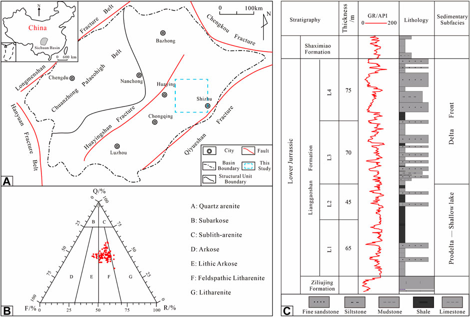
FIGURE 1. Study area (A), stratigraphy (B) and petrological characteristics of Lianggaoshan Formation (C).
The Lianggaoshan Formation in the Fuling area developed a delta-lacustrine depositional system that is mainly influenced by the provenance of the northeast and southwest (Li et al., 2017). During the deposition periods of L1 and L2 members in the Fuling area, the surface of the lake was rising, the process was mainly retrogradation, and shoreline and shallow lake deposit systems were developed. L1 and L2 are mainly black and gray-black shale interbedded with thin gray siltstone. During the deposition periods of L3 and L4 members, the surface of the lake was declining, the process was mainly progradation, delta front deposit systems were developed, and underwater distributary channels were the dominant sand bodies. L3 and L4 are mainly gray fine sandstone and siltstone interbedded with black shale (Zhang et al., 2019). The grain sizes of the L3 and L4 members are coarser than those of the L1 and L2 members, and they are the main reservoirs of the Lianggaoshan Formation in the Fuling area.
3 Data and methods
3.1 Data
The wireline log data and core diagenetic facies types were the main data used for the diagenetic facies prediction in this study. The well cores of the Lianggaoshan Formation in the Fuling area are scare, but the core length of the Lianggaoshan Formation in the FL1 well is large. Thus, the cores of the Lianggaoshan Formation in the FL1 well were intensively and continuously collected and used to determine the diagenetic facies types and logging values. A total of 120 thin sections were made from 2395.00 to 2441.00 m in the FL1 well, with an average of 1 thin section per 0.38 m. The sample density of the logging curves was 0.125 m/sample, and thin sections (0.03 mm) were prepared by impregnation with blue epoxy under vacuum. The composition, structure, and petrologic textural of the 120 samples were determined using a polarizing microscope (A1, Zeiss) and were checked at 400 points/sample. The porosity, permeability, and density of the samples were measured according to GB/T29172-2012 (core analysis method) using a helium porosity measurement instrument (3020-062-00048418), a permeability measurement instrument (DX-07G-00040825), and a dry distillation apparatus (GLY-II-00048478). To determine the types of diagenetic minerals and facies, 41 cathodoluminescence thin sections were prepared and analyzed using a cathodoluminescence microscope (Q00040897) according to SY/T5916-2013 (mineral cathodoluminescence identification method). The pore throat characteristics of 37 samples were analyzed according to GB/T 29171-2012 (capillary pressure curve of rock measured standard). The diagenetic minerals, morphology, composition, and type of the 41 samples were analyzed according to SY/T5162-1997 (SEM method for rock samples), which were measured using a field emission scanning electron microscope (FEI-Quantan 250 FEG) and X-ray energy spectrometer (Oxford-INCa X-MAX 20). The skeleton grains and clay composition of 31 samples were analyzed using XRD. In addition, all the above analyses were combined to determine the relative timing of diagenetic events. It is important to note that the logging values of the 120 samples, such as resistivity logging (RLLD and RLLS), natural potential logging (SP), gamma ray logging (GR), acoustic transit time logging (AC), compensated neutron log(CNL), volume density logging (DEN), and diagenetic facies determined by the above analyses, were used as labels. The logging values and diagenetic facies were important data in the dataset for training the machine learning algorithm.
3.2 Method
3.2.1 K-nearest neighbor
KNN means that each sample can be represented by its K-nearest neighbor values (Lai et al., 2021). Euclidean distance is used to measure the degree of similarity between samples, and the larger the distance, the less similar it is. The Euclidean distance between any two points in space can be written as:
where Dist is the Euclidean distance, xi is the sample eigenvector matrix of the labeled dataset, and yi is the sample eigenvector matrix of the point to be predicted.
When the diagenetic facies type of any point named A in the space was judged, all the Euclidean distances between point A and a point in the dataset were calculated using Eq. 1, and then K points were selected in ascending order of Euclidean distance. Point A has the highest number of K points; for example, in Figure 2A, when K is selected as 5, the sample point of the green square is identified as Type A. For K = 7, the sample point is determined to be Type B; therefore, the KNN algorithm has high requirements for the equilibrium of the sample points and the value of K, and it needs to carefully judge the number of different types of samples and the value of K during classification and prediction.
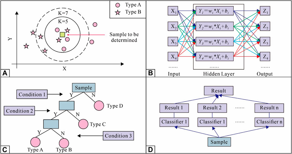
FIGURE 2. Workflow of different algorithms [(A) is the workflow of KNN; (B) is the workflow of BPNN; (C) the workflow of decision tree; (D) is the workflow of random forests].
3.2.2 Back propagation neural networks
A BPNN is a type of multilayer back propagation network that transforms all nonlinear and linear problems into linear problems for calculation, and usually includes an input layer, hidden layer, and output layer (Li et al., 2022). When Xi is a multidimensional vector, the calculation expression for the first hidden layer can be written as:
where Yi is the calculation result for each neuron in the hidden layer, wi is the weight, and bi is the bias.
The principle of a BPNN is shown in Figure 2B. The gradient descent method was used to establish the model in this study, and the learning, training, and adjustment were carried out through a fully connected neural network to finally achieve the purpose of predicting diagenetic facies. When there was an error between the result obtained by forward propagation and the actual result, the error was fed back to each neuron system in the hidden layer using the gradient search technique through back propagation. This was done to adjust their respective weights to make the error variance between the actual output and the expected output the smallest. The BPNN construction process can be divided into four steps: 1) Normalize the sample data and then set the training and prediction data. 2) Configure the network parameter (training time, number of hidden layers, etc.). 3) Establish and train the BPNN model to improve its prediction accuracy. 4) Use the trained BPNN model to predict diagenetic facies without core samples. The disadvantage of the BPNN is that with an increase in the number of neurons, the amount of computation increases rapidly, and the internal weight and bias given to the hidden layer usually have no physical meaning, which causes poor interpretability of the BPNN.
3.2.3 Decision tree
The flow chart of the decision tree is similar to that of a tree, including a root node, multiple internal nodes, and leaf nodes (Zhou et al., 2019; Liu and Liu, 2021). The root node represents the total sample dataset, and the different leaf nodes represent different categories of sample diagenetic facies. The internal node is located between the root and leaf nodes. The decision tree completes sample classification from the root node to the leaf node so that the decision tree model can deduce classification rules from a group of random and unordered classified samples (Figure 2C). The decision tree algorithm uses information entropy to select optimal classification features, and the samples gradually become clear and separable. The smaller the information entropy, the higher the sample classification purity.
3.2.4 Random forest model
The random forest model is composed of multiple classifiers, which are mainly decision trees. The prediction results of stochastic forest classification were generated by voting multiple classifiers (Rahimi and Riahi, 2002; Zhou et al., 2019) (Figure 2D). The process of constructing the random forest learning model is as follows: 1) n subsets of data were extracted by the self-sampling method based on the diagenetic facies dataset, and n decision tree models were constructed for classification. 2) The random forest model was combined with n decision trees, which were independent of each other without considering weights. 3) The random forest model was used to classify the diagenetic facies, and the classification results of all classifiers were counted. The type with the highest frequency was selected as the classification result. Thus, the number and depth of decision trees can have a great impact on the prediction accuracy of random forest models and are the main parameters for building a random forest learning model.
4 Classification and prediction of diagenetic facies
4.1 The characteristics of petrological and diagenesis
The highest, lowest, and average contents of quartz, feldspar, and rock fragments of tight sandstone in the Lianggaoshan Formation are 60%, 34%, and 47.36%; 32%, 12%, and 20.89%; and 47%, 22%, and 31.75%, respectively. Thus, the tight sandstone of the Lianggaoshan Formation is dominated by lithic arkose with a small amount of arkose and litharenite (Figure 1B) and its burial depth is medium. Under the influence of compaction and cementation, the porosity of the reservoir decreased or disappeared and was generally small, mainly in the range of 0%–8% (Figure 3). The tight sandstone in the Lianggaoshan Formation experienced different degrees of compaction, cementation, dissolution, and metasomatism, which resulted in significant differences in the physical properties of tight sandstone reservoirs.
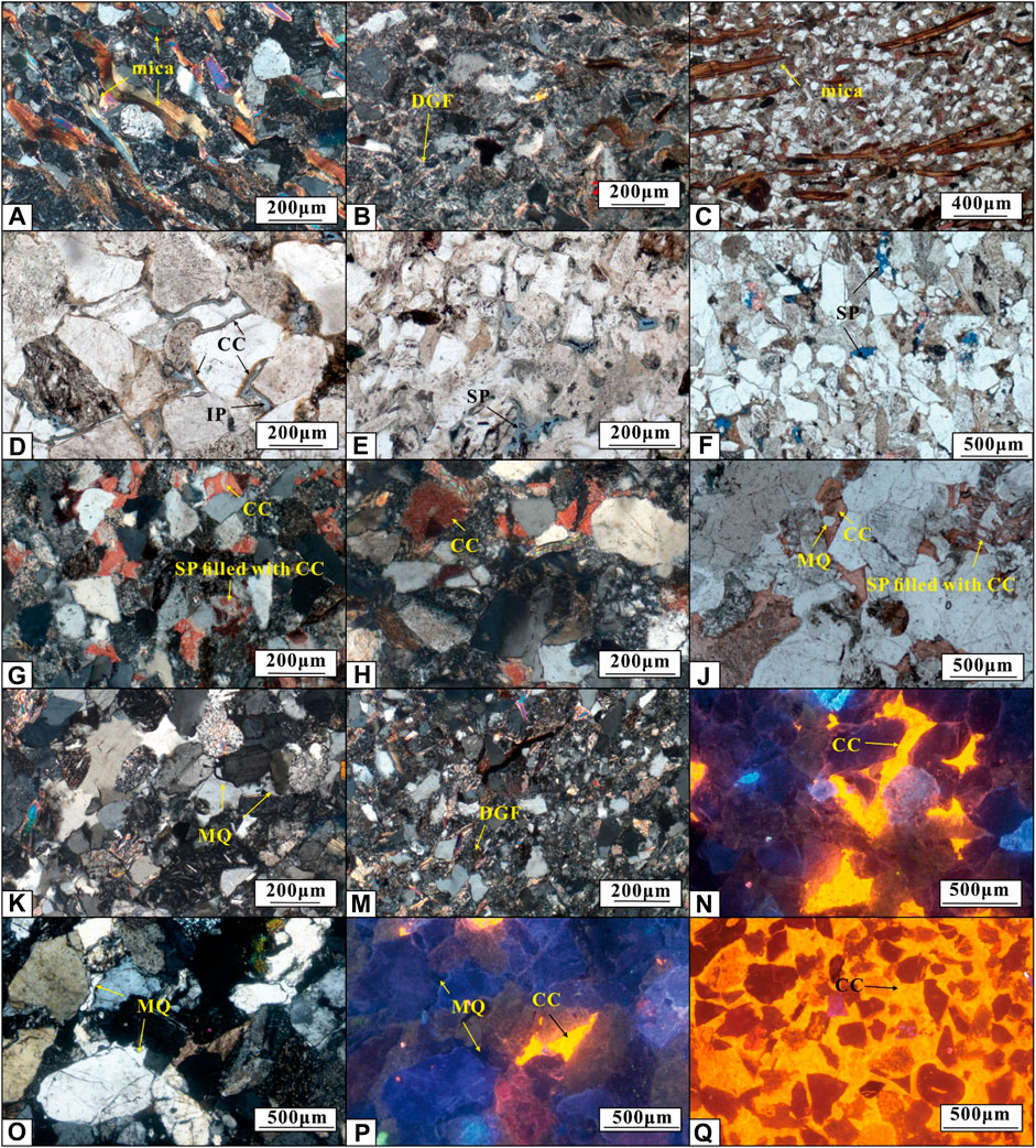
FIGURE 3. Microscopic characteristics of diagenesis [(A–C) is the ductile grain deformation (2408.70, 2495.55, and 2546.50 m); (D) is the chlorite coating and primary porosity (2425.57 m); (E,F) are the dissolution of debris grains (2412.25 and 2465.04 m); (G,H,J,K) are carbonate cementation and microcrystalline quartz cementation (2496.00, 2455.92, 2429.01, and 2399.25 m); (M–Q) are the microscopic characteristics of carbonate cementation and microcrystalline quartz cements in cathode luminescence (2396.65, 2428.07, 2428.07, 2428.07 and 2422.03 m)].
4.1.1 Cementation
There are various types of cement in the tight sandstone of the Lianggaoshan Formation, including siliceous (Figure 3O), carbonate (Figures 3G,H,J,N,P,Q), and clay (Figure 3D). Siliceous cementation is not well-developed and is not the main factor in the porosity reduction of tight sandstone in the Liangshan Formation. Carbonate cementation was strong in some samples, which showed basement cementation, and its main color was red after staining with potassium ferricyanide and alizarin red (Figures 3G,H,J). Carbonate cements show a high white interference color under orthogonal light and orange-red under cathode luminescence (Figures 3N,P,Q). In addition, the dissolution of carbonate cements was observed under a scanning electron microscope, and the results of the energy spectrum showed that Ca, O, and C were dominant (Figure 4B). Based on the aforementioned characteristics, calcite cement is the main carbonate cement. Although ferric calcite and ferrite cements are also found in some samples, the content is generally low and is not the main factor causing porosity reduction in the tight sandstone of the Lianggaoshan Formation. It is difficult to reflect this information in logging curves when the contents of ferric calcite and ferrite cements are low; therefore, this study did not discuss them during the burial process.
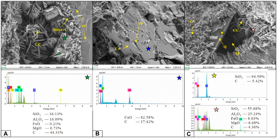
FIGURE 4. Types of cement and results of energy spectrum analysis [(A) primary pores were filled with clay minerals, 2465.10 m; (B) carbonate cements were dissolved, 2487.80 m; (C) chlorite coating were developed on the surface of quartz grain, 2458.90 m. CC is chlorite coating; SP is secondary pores, IP is primary pores; Q is quartz; Ca is calcite cement].
Clay cementation is widely observed in the tight sandstone of the Lianggaoshan Formation, and the types of clay cements include chlorite coating (Figure 3D), illite (I), and illite and montmorillonite mixed layers (I/S), which originate from feldspar and other lithic fragments alterations (Figure 5B). Chlorite coating is usually distributed on the surface of quartz grains, which inhibits the enlargement of quartz and has a strong protective effect on the primary pores (Figures 3D, 5C,D). The results of the SEM and energy spectrum analysis show that I and I/S are often distributed on the edge of feldspar and debris particles, which are the alteration products of skeleton particles during the process of dissolution (Figures 4A, 5B). In addition, clay cements generally develop more intergranular micropores, but they also block the throats, which reduces permeability. Thus, the influence of clay cementation on the physical properties of the reservoir was two-fold. They can protect the primary pores and maintain high porosity, but at the same time, they can block the throat and reduce the permeability of tight sandstone.
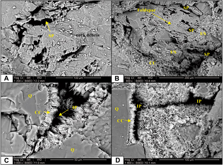
FIGURE 5. Pore types in tight sandstone of the Lianggaoshan Formation [(A) is the dissolution of debris grains, 2395.87 m; (B) is the dissolution of feldspar, 2424.04 m; (C,D) are the chlorite coating on the quartz grains, clay minerals fill the initial pores, and intergranular micropores of clay mineral develop, 2414.85 and 2439.38 m. SP is secondary pores, IP is initial pores, Q is quartz grains, CC is chlorite coating, I/S is illite and montmorillonite layer].
4.1.2 Compaction
The compaction of tight sandstone in the Lianggaoshan Formation is strong, and the contact relationship between grains is dominated by point-line and line-concave contacts (Figures 3A–C,E,K,M,N). In addition, the sedimentary facies of the Lianggaoshan Formation are delta front and front delta, and the ductile grain content, such as mica content, in some samples is high, which shows strong plastic deformation and causes porosity loss (Figures 3A–C,M). Thus, compaction is another important factor leading to porosity loss, and the physical properties are poor, particularly in samples with highly ductile grains.
4.1.3 Dissolution
Dissolution is one of the main factors causing a pore increase in the tight sandstone of the Lianggaoshan Formation, which is reflected in the dissolution of feldspar grains and lithic fragments by organic acids, forming ingrain or intergrain dissolution pores (Figure 3F). In addition, the dissolution of calcite cement also occurred because of the presence of organic acids (Figure 4B). Some feldspar dissolution pores were filled with calcite cements (Figure 3J) and some were filled with bitumen (Figures 3F, 4A). Thus, the dissolution of skeleton grains and carbonate cements is an important condition for improving the physical properties of tight sandstone in the Lianggaoshan Formation.
4.1.4 Others
There are many other diagenetic processes in the tight sandstone of the Lianggaoshan Formation, such as authigenic pyrite cementation, carbonate metasomatism feldspar particles, and mutual transformation of clay minerals. However, these did not play a crucial role in the evolution of the physical properties of this sandstone and cannot be used as an important basis for naming diagenetic facies.
4.2 Diagenetic facies and their physical properties
The relationships between clay cement content, chlorite coating content, secondary porosity, porosity, and permeability content are shown in Figure 6. The cement content in the tight sandstone of the Lianggaoshan Formation has a significant influence on the physical properties of the reservoir. When the cement content was more than 10%, the porosity of this sandstone was almost less than 2% (Figure 6A). The higher the relative content of chlorite, the higher the porosity and the lower the permeability of the sandstone (Figures 6B,D). Chlorite protects the primary pores of the reservoir, but also blocks the throat and has a dual effect on reservoir properties, which is also shown in the SEM images (Figures 5C,D). In addition, the relationship between secondary porosity and measured porosity is bilinear, indicating that there are two types of high-quality reservoirs in the Lianggaoshan Formation (Figure 6C). In addition, SEM observation results show that there are two different pore types in tight sandstone: secondary pores, which are formed by the dissolution of feldspar and lithic fragments (Figures 5A,B), and primary pores, which are preserved during burial due to chlorite coating (Figures 5C,D).
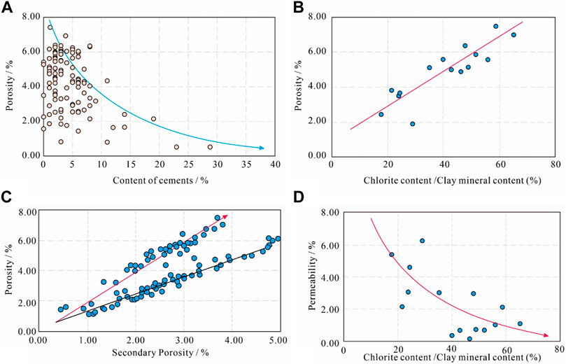
FIGURE 6. The influence of cements on porosity [(A) is the relationship between porosity and content of cements; (B) is the relationship between porosity and chlorite content/clay content; (C) is the relationship between porosity and secondary porosity; (D) is the relationship between porosity and permeability and chlorite content/clay content].
Based on diagenetic minerals, pore types, and relationships between cement content and porosity, four types of diagenetic facies of the Lianggaoshan Formation are recognized: carbonate cemented (CCF), tightly compacted (TCF), chlorite coating and clay mineral filling (CCCMFF), and dissolution facies (DF).
For the CCCMFF, the primary pores developed, porosity was between 4.91% and 7.91%, the average porosity and permeability were 6.3% and 0.0029 mD, respectively. The porosity of this facies was the highest, the permeability was medium, and the physical properties of the reservoir were good (Figure 7).
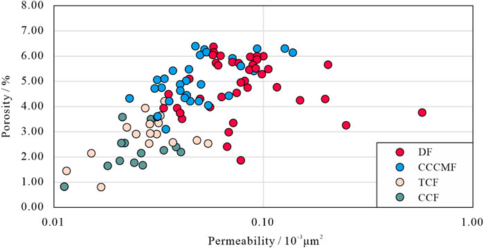
FIGURE 7. Physical properties of four diagenesis facies.
For the DF, secondary pores developed, porosity was between 2.83% and 5.63%, and the average porosity and permeability were 4.8% and 0.089 mD, respectively. The reservoir properties were relatively good (Figure 7).
For the TCF, the clay and ductile grain contents were high, the porosity varied poorly in the range of 1.13% and 2.42%, the average porosity and permeability were 2.2% and 0.011 mD, respectively, and the reservoir properties were relatively poor (Figure 7).
Most of the CCF are basement cementation, and small samples are pore cementation. The porosity ranged between 0.18% and 2.08%, the average porosity and permeability were 1.6% and 0.007 mD, respectively, and the reservoir properties were poor (Figure 7).
The Hg injection curves of the four types of diagenetic facies are shown in Figure 8. The absolute values of the entry pressure of the four types have little difference, mainly ranging from 1.0 to 4.0 MPa, but there are still some differences. The entry pressure of the DF is the lowest, followed by CCCMFF, TCF, and CCF. Therefore, the presence of clay cements significantly blocks the throat and the pressure usually needs to overcome the intergranular micropores in the clay cements to enter the larger primary pores. Maximum mercury intake saturation and mercury desaturation saturation had similar characteristics. In general, maximum mercury intake saturation and mercury desaturation saturation of DF are maximal, followed by CCCMFF, while those of TCF and CCF are relatively low.
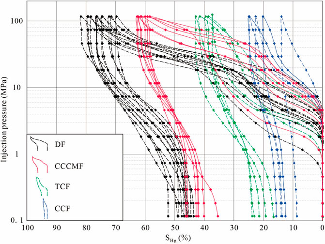
FIGURE 8. Pore throat characteristics of four diagenesis facies.
4.3 Logging values and prediction of four diagenetic facies
4.3.1 Logging values of four diagenetic facies
Conventional logs are sensitive to changes in diagenetic minerals and diagenetic facies types, which include natural gamma rays (GR) and three porosity logs, that is, acoustic transit time (AC), bulk density (DEN), compensated neutron (CNL), and resistivity logs (LLS and LLD) (Lai et al., 2016; Cui et al., 2017). Based on the logging response characteristics of the 120 core samples, six sensitive logs were selected for diagenetic facies prediction: DEN, CNL, AC, GR, LLD, and LLS (Figure 9).
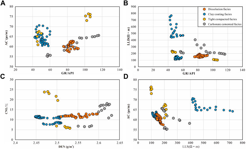
FIGURE 9. The characteristics of logging values of four diagenetic facies.(A) Data points of four diagenetic facies in the AC-GR crossplot. (B) Data points of four diagenetic facies in the LLD-GR crossplot. (C) Data points of four diagenetic facies in the CNL-DEN crossplot. (D) Data points of four diagenetic facies in the AC-LLS crossplot.
For CCCMFF, GR is lower than 63 API, DEN is between 2.41 and 2.63 g/cm3, AC is between 53 and 76 μs/m, and CNL is between 5.9% and 11.8%. Owing to the existence of primary and secondary pores, the resistivity values were between 110 and 720 Ω•m (Figures 9, 10).
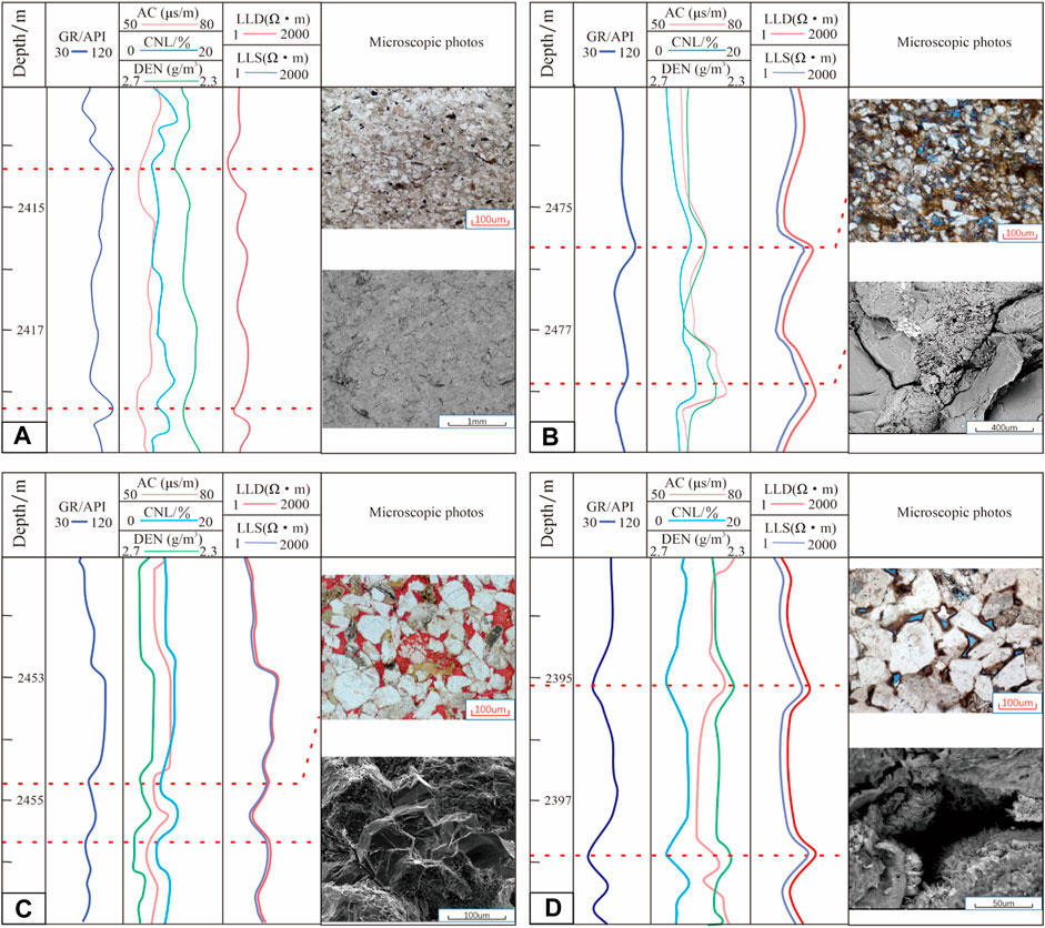
FIGURE 10. Logging values of four diagenetic facies [(A) is TCF, (B) is DF; (C) is CCF; (D) is CCCMFF].
For DF, GR is higher than 75 API, DEN is between 2.51 and 2.60 g/cm3, AC is between 57 and 63 μs/m, and CNL is between 10.9% and 13.00%. Owing to the existence of secondary pores, the resistivity values were between 138 and 192 Ω•m (Figures 9, 10).
For CCF, GR is between 56.6 and 116.2 API, DEN is between 2.54 and 2.64 g/cm3, AC is between 180.4 and 393.7 μs/m, and CNL is between 6.5% and 18.6%. Owing to the existence of secondary pores, the resistivity values were between 180 and 406 Ω•m (Figures 9, 10).
For TCF, GR is between 45.2 and 106.4 API, DEN is between 2.47 and 2.54 g/cm3, AC is between 60.9 and 76.4 μs/m, and CNL is between 5.7% and 24.1%. Owing to the existence of secondary pores, the resistivity values were between 95 and 235 Ω•m (Figures 9, 10).
In general, the CCCMFF have high AC, LLD, LLS, and low GR, DEN, and CNL; the DF have high GR, DEN, CNL, and low AC, LLD, and LLS; the CCF have high GR, LLD, LLS, DEN, and low CNL, AC; and the TCF have AC, GR, CNL, and low LLD, LLS, and DEN (Figure 10).
4.3.2 Prediction of four diagenetic facies
A total of 120 logging data points and diagenetic facies types were selected as the dataset. Among these samples there were 26 CCCMFF, 20 DF, 48 TCF, and 26 CCF. Four machine learning methods were used to construct the diagenetic facies prediction model by using logging data and diagenetic facies type as the independent and dependent variable sets, respectively. In addition, all logging data were standardized.
4.3.2.1 K-nearest neighbor
The K value has a significant influence on the KNN prediction results; thus, the value range of K was set from 1 to 16, and the dataset was divided into training and test sets. The relationship between the predicted accuracy of the KNN and the change in the K value is plotted in Figure 11. The results show that the prediction accuracy of diagenetic facies based on the KNN decreases gradually with an increase in the K value. In the logging prediction of tight sandstone diagenetic facies, the smaller the K value, the lower the number of nearest neighbors selected, and the higher the accuracy of the diagenetic prediction. On the contrary, the larger the number of nearest neighbors, the larger the value of K, and the more prone it is to overfitting, that is, a lower accuracy.
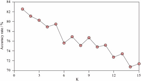
FIGURE 11. The diagenetic facies predicted results by KNN.
When the K value was five, the predicted accuracy rate exhibited a partial upward trend. In addition, there are four types of diagenetic facies in the tight sandstone of the Lianggaoshan Formation, and the K value of 5 is greater than the number of diagenetic facies. The predicted rater of the diagenetic facies was highest and equal to 81.32% when the value of K was 5. Thus, the KNN predicted model was finally constructed with k = 5 to identify diagenetic facies.
4.3.2.2 Back propagation neural networks
The sample data of the diagenetic facies were divided into a training set and a test set at a ratio of 3:1. The number of cycles was 20000, and the predicted accuracy of the BPNN was 95.83%, the results of which are shown in Figure 12.
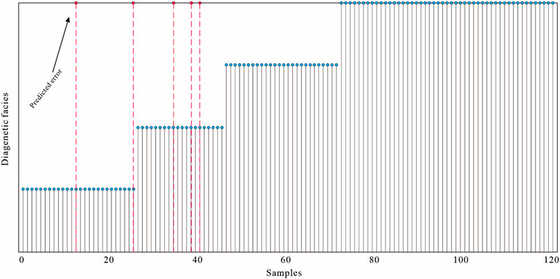
FIGURE 12. The diagenetic facies predicted results by BPNN.
The predicted results of CCF and TCF were the same as the actual results, and there was no prediction error when the BPNN model was used. However, the predicted results of CCCMFF and DF had two and three samples that were incorrectly predicted, respectively. They were all predicted to be tightly compacted facies, but the overall prediction accuracy was high.
4.3.2.3 Decision tree
The established process of the decision tree model is the process of completing optimal classification. The purpose of a decision tree prediction is to ensure that each leaf node contains only one type of diagenetic facies, so the depth of the decision tree is the main control parameter of the decision tree model. Therefore, the depth of the decision tree was selected to vary from 1 to 15, the dataset was used for training, and the predicted accuracy of the decision tree was analyzed. The results show that the predicted accuracy of the decision tree first increases and then stabilizes with an increase in the depth of the decision tree (Figure 13). When the depth of the decision tree is 3, the predicted accuracy is 89.32%, which then fluctuates and stays near the highest value. When the depth selection of the decision tree is too large, the model will overfit, which reduces the recognition accuracy and interpretability of the decision tree model. Thus, the depth of the decision tree was selected as 3 to build the predicted model, and the diagenetic facies of the tight sandstone of the Lianggaoshan Formation was predicted.
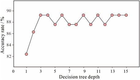
FIGURE 13. The diagenetic facies predicted results by decision tree.
4.3.2.4 Random forests
The classifiers used in random forests are decision trees, and the number and depth of decision trees in random forests are important factors affecting the prediction accuracy of the random forest model. The number of decision trees ranges from 1 to 100, and the depth of the decision tree ranges from 1 to 50. The relationship between the predicted accuracy and the decision tree number and depth is shown in Figure 14.
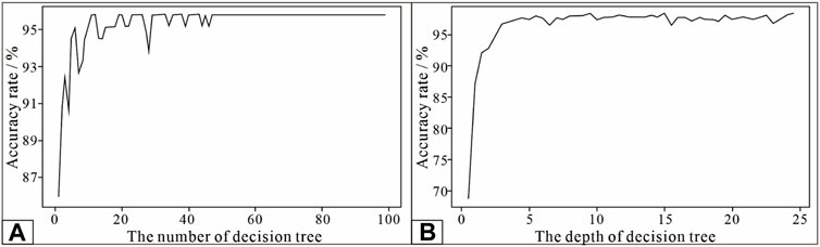
FIGURE 14. The diagenetic facies predicted results by random forests. (A) The relationship between predicted accuracy and the number of decisiontree. (B) The relationship between predicted accuracy and the depth of decision tree.
The prediction accuracy of the random forest continues to improve with an increase in the number and depth of decision trees. When the number of decision trees was equal to 50 and the depth of decision was equal to three, the predicted accuracy was the highest. Subsequently, the predicted accuracy gradually stabilized, which indicates that the random forest has a strong ability to resist overfitting, and parameters that are too large will not have a significant impact on the random forest model. In addition, if the parameters of the random forest are too large, this will lead to an increase in the calculation and time, thus affecting the operation efficiency (Figure 14). Thus, the number of decision trees was set to 50, and the depth of the decision tree was set to 3 to construct the random forest model. The prediction accuracy of the diagenetic facies model was 97.5%.
5 Discussion
5.1 Comparison applications of machine learning models in well log-lithofacies predictions
The predicted basis and calculation methods of the four types of machine learning methods for diagenetic facies logging prediction are different. The KNN adopts the prediction principle of Euclidean distance, the BPNN adopts the core idea of gradient descent, the decision tree uses information entropy as the main predicted basis, and the random forest is a voting method using multiple decision trees. The predicted accuracies of the four methods are ranked from high to low as follows: random forest, BPNN, decision tree, and KNN. The predicted accuracy of the random forest was the highest at 97.5%, whereas that of KNN was the lowest at 81.32%.
The predicted accuracies of the four types of diagenetic facies using different machine learning methods are also different. In general, the predicted accuracy of the TCF was the highest, whereas that of the DF was the lowest. The main reason for this is that the number of TCF samples is relatively larger than that of dissolution facies samples, which leads to some of these being easily misjudged as TCF. KNN had the largest difference in the predicted accuracy of different diagenetic facies (11.82%), and random forests had the smallest difference in the predicted accuracy of different diagenetic facies (5.00%).
Four machine learning methods, KNN, decision tree, BPNN, and random forest, were used to predict the diagenetic facies in the 2437–2462 m section of well FL1, and the prediction results are shown in Figure 15. The diagenetic facies types predicted by the random forest had the best match with the diagenetic facies type calibrated by core samples. In addition, the matching relationship between the random forest prediction results and the physical properties was also good, which is in accordance with the results of the physical characteristics of different diagenetic facies based on core analysis. The prediction results of the BPNN are good, while those of the decision tree and KNN are relatively poor, and some prediction results do not meet the core analysis data. Compared with the random forest model, the TCF predicted by the KNN, decision tree, and BPNN are relatively rich, and that of the dissolution facies is relatively poor. The reason for these results may be that the number of TCF samples is almost twice that of the dissolution facies. The sample data are unbalanced, causing the KNN, decision tree, and BPNN methods to easily misjudge the DF as TCF, which makes the predicted accuracy of the KNN, decision tree, and BPNN methods lower than that of the random forest. The difference in the predicted accuracy between different diagenetic facies by the four machine methods also indicates this feature (Table 1). Based on the above data and comparison results, the random forest algorithm is more suitable for the prediction of diagenetic facies of tight sandstone in the Lianggaoshan Formation, which has few geological sample points with poor equilibrium.
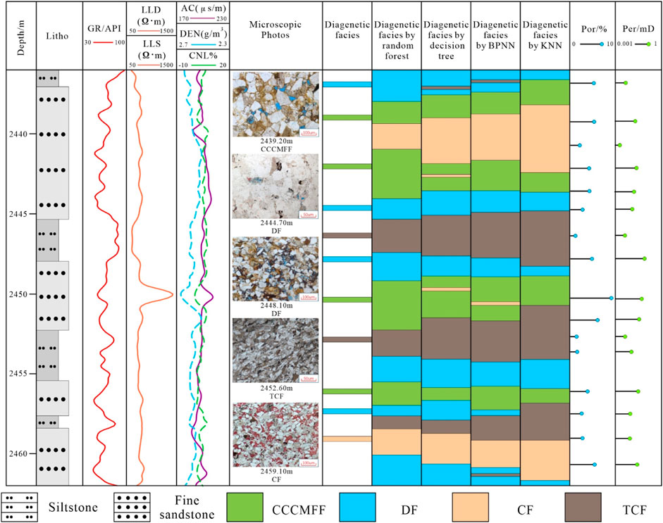
FIGURE 15. Diagenetic facies logging identification results in the T1 well (Note: CCCMFF is chlorite coating and clay mineral filling facies; DF is dissolution facies; CF is carbonate-cemented facies; TCF is tightly compacted facies).
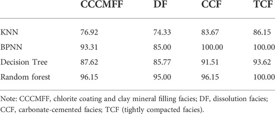
TABLE 1. Statistical table of identification accuracy of different diagenetic facies.
In addition, the KNN method has a poor generalization ability and is suitable for logging data of diagenetic facies with low complexity and low crossover. The BPNN has a strong generalization ability, but belongs to the “black box,” in that the classification process is not visible, the geological meaning of the model parameters is not clear, and it is suitable for the processing of diagenetic facies data complex and high degree of clutter. A decision tree can visualize the classification process of diagenetic facies, but it is easily affected by the imbalance of data samples; therefore, it is suitable for diagenetic facies data with clear classification criteria. The random forest method represents an ensemble learning method that can balance the sample error, improve the prediction accuracy, and has a wide range of applications.
5.2 Diagenetic facies characteristics and favorable tight reservoir prediction
The predicted results (Figure 16) of the four machine learning methods show that chlorite coating and clay mineral filling facies have high LLD, AC, and low GR; dissolution facies have high GR and CNL; tightly compacted facies have low LLD, LLS, and high GR; and carbonate-cemented facies have high LLD and low AC. The average porosity and permeability of the chlorite coating and clay mineral filling facies were 6.3% and 0.0029 mD, respectively. The average porosity and permeability of the dissolution facies were 4.80% and 0.089 mD, respectively. The physical properties of the tight compacted facies and carbonate-cemented facies were relatively poor. Thus, there are two favorable diagenetic facies in the tight sandstone of the Lianggaoshan Formation: CCCMFF with relatively developed primary pores, and DF with secondary pores.
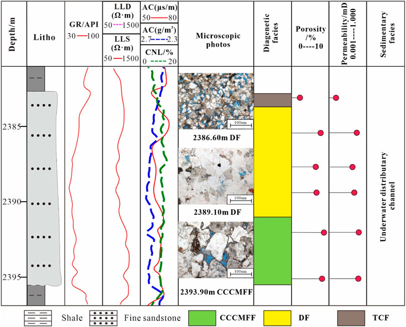
FIGURE 16. Diagenetic facies distribution of distributary channel (Note: CCCMFF is chlorite coating and clay mineral filling facies; DF is dissolution facies; TCF is tightly compacted facies).
Although the machine learning method can be used to predict the diagenetic facies of the whole well using logging data, the accuracy of diagenetic prediction can be improved continuously, even reaching 100%. However, the number of wells in the exploration area is small, and the quality of seismic data poor. These actual geological data cannot be compensated for by the advantages of the machine learning algorithm. Through the analysis of the logging diagenetic facies in sand bodies of typical sedimentary facies, a systematic relationship between diagenetic facies and sedimentary facies was established. Using sedimentary models and diagenetic facies distribution laws to predict favorable reservoirs may be an important future research field for machine learning. For example, the sedimentary microfacies of well FY1 between 2383.00 and 2395.50 m is underwater distributary channel, with a thickness of about 12.50 m. In the sand body of the underwater distributary channel, the grain size gradually becomes finer from bottom to top. The diagenetic facies prediction results by the random forest show that the CCCMFF and DF are in the middle and at the bottom, respectively, and TCF are on the top of the sand bodies. In addition, the porosity and permeability exhibited a gradual deterioration trend from bottom to top. The results show that the diagenetic facies of the underwater distributary channel sand bodies are different, and the CCCMFF, and DF, which represent favorable reservoirs, are distributed in the middle and lower parts of the distributary channel sand bodies. In other words, sedimentary facies controlled the distribution of diagenetic facies. For exploration areas with less well data, sedimentary facies can be used to predict favorable reservoir distribution. For exploration areas with more well data and core samples, the systematic diagenetic facies prediction can be executed by machine learning methods using logging data, and then a geostatistics method sedimentary model can be used to predict the favorable diagenetic facies distribution in the study area. Zhao et al. (2022) provided a case study of this geological condition in the tight sandstone of the Xujiahe Formation in the Sichuan Basin. For the Fuling area, the relationship between the sedimentary facies model and diagenetic facies may be the main method for predicting favorable areas in future studies.
In summary, a suitable machine method should be selected based on the actual geological conditions when using logging data to predict the diagenetic facies so as to improve the prediction accuracy and save time and labor costs. The random forest composited with the decision tree classifier has high diagenetic facies prediction accuracy in the tight sandstone, the predicted process can be interpreted strongly, and the influence of sample data balance can be avoided. In the study area, with more well data and core samples, the BPNN may have a better predicted result.
6 Conclusion
(1) The tight sandstone of the Lianggaoshan Formation is dominated by lithic arkose with a small amount of arkose and litharenite. There are two different pore types in the tight sandstone: secondary pores, which are formed by the dissolution of feldspar grains and lithic fragments, and primary pores, which are preserved during burial due to chlorite coating.
(2) Four types of diagenetic facies are recognized: carbonate cemented (CCF), tightly compacted (TCF), chlorite coating and clay mineral filling (CCCMFF), and dissolution facies (DF). Primary pores develop in the CCCMFF, and secondary pores develop in the DF. The average porosity and permeability of the CCCMFF were 6.3% and 0.0029 mD, respectively. The average porosity and permeability of the DF were 4.80% and 0.089 mD, respectively. The physical properties of the TCF and CCF were poor.
(3) A diagenetic facies prediction model with four machine learning methods was established, where the random forest had the highest prediction accuracy of 97.5%, followed by the BPNN, decision tree, and KNN methods. The sample data are unbalanced, causing the predicted accuracy of the KNN, decision tree, and BPNN methods to be lower than that of the random forest.
Data availability statement
The original contributions presented in the study are included in the article/supplementary material, further inquiries can be directed to the corresponding author.
Author contributions
LZ: conceptualization, methodology, investigation, data curation, methodology, writing—original draft, writing—review and editing, and funding acquisition; YY: conceptualization, methodology, investigation, data curation, and supervision. All other authors listed have made a substantial, direct, and intellectual contribution to the work and approved it for publication.
Funding
This study was supported by the Strategic Priority Research Program of the Chinese Academy of Sciences (XDA14010202).
Acknowledgments
We’d also like to thank the reviewers and executive editor for their insightful comments and suggestions regarding our manuscript. In addition, we would like to thank SINOPEC Exploration Company for providing us with some analytical data.
Conflict of interest
Authors WW and CL were employed by Sinopec Exploration Company. Author SJ was employed by Shengli Oil Production Company.
The remaining authors declare that the research was conducted in the absence of any commercial or financial relationships that could be construed as a potential conflict of interest.
Publisher’s note
All claims expressed in this article are solely those of the authors and do not necessarily represent those of their affiliated organizations, or those of the publisher, the editors and the reviewers. Any product that may be evaluated in this article, or claim that may be made by its manufacturer, is not guaranteed or endorsed by the publisher.
References
Abedini, A., and Calagari, A. A. (2017). Geochemistry of claystones of the Ruteh Formation, NW Iran: Implications for provenance, source-area weathering, and paleo-redox conditions. njma. 194, 107–123. doi:10.1127/njma/2017/0040
Abedini, A., Khsravi, M., and Dill, H. G. (2020a). Rare Earth element geochemical characteristics of the late Permian Badamlu karst bauxite deposit, NW Iran. J. Afr. Earth Sci. 172, 103974. doi:10.1016/j.jafrearsci.2020.103974
Abedini, A., Rezaei Azizi, M., and Calagari, A. A. (2018). Lanthanide tetrad effect in limestone: A tool to environment analysis of the ruteh formation, NW Iran. Acta Geodyn. Geromaterialia 15, 229–246. doi:10.13168/AGG.2018.0017
Abedini, A., Rezaei Azizi, M., and Dill, H. G. (2020b). Formation mechanisms of lanthanide tetrad effect in limestones: An example from arbanos district, NW Iran. Carbonates Evaporites 35, 1–18. doi:10.1007/s13146-019-00533-z
Bhattacharya, S., Ghahfarokhi, P. K., Carr, T. R., and Pantaleone, S. (2019). Application of predictive data analytics to model daily hydrocarbon production using petrophysical, geomechanical, fiber-optic, completions, and surface data: A case study from the marcellus shale, North America. J. Pet. Sci. Eng. 176, 702–715. doi:10.1016/j.petrol.2019.01.013
Bjørlykke, K., and Jahren, J. (2012). Open or closed geochemical systems during diagenesis in sedimentary basins: Constraints on mass transfer during diagenesis and the prediction of porosity in sandstone and carbonate reservoirs. Am. Assoc. Pet. Geol. Bull. 96 (12), 2193–2214. doi:10.1306/04301211139
Cao, B., Luo, X., Zhang, L., Sui, F., Lin, H., and Lei, Y. (2017). Diagenetic evolution of deep sandstones and multiple-stage oil entrapment: A case study from the lower jurassic sangonghe Formation in the fukang sag, central junggar basin (NW China). J. Pet. Sci. Eng. 152, 136–155. doi:10.1016/j.petrol.2017.02.019
Chauhan, S., Ruhaak, W., Khan, F., Enzmann, F., Mielke, P., Kersten, M., et al. (2015). Processing of rock core microtomography images: Using seven different machine-learning algorithms. Comput. Geosci. 86, 120–128. doi:10.1016/j.cageo.2015.10.013
Cuddy, S., and Glover, P. W. J. (2002). The application of fuzzy logic and genetic algorithms to reservoir characterization and modeling, 80. Springer, 219–242. doi:10.1007/978-3-7908-1807-9_1
Cui, Y., Wang, G., Jones, S. J., Zhou, Z., Ran, Y., Lai, J., et al. (2017). Prediction of diagenetic facies using well logs–a case study from the upper triassic yanchang formation, ordos basin, China. Mar. Pet. Geol. 81, 50–65. doi:10.1016/j.marpetgeo.2017.01.001
Dai, J. X., Ni, Y. Y., and Wu, X. Q. (2012). Tight gas in China and its significance in exploration and exploitation. Pet. Explor. Dev. 39 (3), 277–284. doi:10.1016/S1876-3804(12)60043-3
De Segonzac, G. D. (1968). The birth and development of the concept of diagenesis (1866- 1966). Earth. Sci. Rev. 4, 153–201. doi:10.1016/0012-8252(68)90149-9
Deng, T., Xu, C., Lang, X., and Doveton, J. (2021). Diagenetic facies classification in the arbuckle formation using deep neural networks. Math. Geosci. 53, 1491–1512. doi:10.1007/s11004-021-09918-0
Dubois, M. K., Bohling, G. C., and Chakrabarti, S. (2007). Comparison of four approaches to a rock facies classification problem. Comput. Geosci. 33 (5), 599–617. doi:10.1016/j.cageo.2006.08.011
Fan, Y., Li, F., Deng, S. R., Chen, Z., Li, G., and Li, J. (2018). Characteristics analysis of diagenetic facies in tight sandstone reservoir and its logging identification. Well Logging Technol. 42 (3), 307–314. doi:10.16489/j.issn.1004-1338.2018.03.011
Fu, G. M., Qin, X. L., Miao, Q., Zhang, T. J., and Yang, J. P. (2009). Division of diagenesis reservoir facies and its control case study of Chang-3 reservoir in Yangchang Formation of Fuxian exploration area in Northern Shaanxi. Min. Sci. Technol. 19 (4), 537–543. doi:10.1016/S1674-5264(09)60101-0
Grigsby, J. D., and Langford, R. P. (1996). Effects of diagenesis on enhanced-resolution bulk density logs in tertiary gulf coast sandstones: An example from the lower vicksburg formation, McAllen ranch field, south Texas. Am. Assoc. Pet. Geol. Bull. 80, 1801–1819. doi:10.1306/64EDA172-1724-11D7-8645000102C1865D
He, J., Wen, X. T., Nie, W. L., Li, L. H., and Yang, J. X. (2020). Fracture zone prediction based on random forest algorithm. Oil Geophys. Prospect. 55 (1), 161–166. doi:10.13810/j.cnki.issn.1000-7210.2020.01.019
Jia, C., Zou, C., Li, J., Li, D., and Zheng, M. (2012). Assessment criteria, main types, basic features and resource prospects of the tight oil in China. Acta Pet. Sin. 33 (3), 343–350. doi:10.7623/syxb201203001
Kassab, M. A., Hassanain, I. M., and Salem, A. M. (2014). Petrography, diagenesis and reservoir characteristics of the pre-cenomanian sandstone, Sheikh Attia area, East Central Sinai, Egypt. J. Afr. Earth Sci. 96 (3), 122–138. doi:10.1016/j.jafrearsci.2014.03.021
Ketzer, J. M., and Morad, S. (2006). Predictive distribution of shallow marine, low porosity (pseudomatrix-rich) sandstones in a sequence stratigraphic framework: Example from the ferron sandstone, upper cretaceous, USA. Mar. Pet. Geol. 23, 29–36. doi:10.1016/j.marpetgeo.2005.05.001
Khalifah, H. A., Glover, P. W. J., and Lorinczi, P. (2020). Permeability prediction and diagenesis in tight carbonates using machine learning techniques. Mar. Pet. Geol. 112, 104096. doi:10.1016/j.marpetgeo.2019.104096
Khan, Z., Ahmad, A. H. M., Sachan, H. K., and Quasim, M. A. (2018). The effects of diagenesis on the reservoir characters in ridge sandstone of jurassic jumara dome, kachchh, Western India. J. Geol. Soc. India 92, 145–156. doi:10.1007/s12594-018-0973-z
Khanam, S., Quasim, M. A., and Ahmad, A. H. M. (2021). Diagenetic control on the distribution of porosity within the depositional facies of Proterozoic Rajgarh Formation, Alwar sub-basin, Northeastern Rajasthan. J. Geol. Soc. India 97, 697–710. doi:10.1007/s12594-021-1752-9
Lai, J., Fan, X., Liu, B., Pang, X., Zhu, S., Xie, W., et al. (2020). Qualitative and quantitative prediction of diagenetic facies via well logs. Mar. Pet. Geol. 120, 104486. doi:10.1016/j.marpetgeo.2020.104486
Lai, J., Fan, X., Pang, X., Zhang, X., Xiao, C., Zhao, X., et al. (2019). Correlating diagenetic facies with well logs (conventional and image) in sandstones: The eocene–oligocene suweiyi formation in dina 2 gasfield, kuqa depression of China. J. Pet. Sci. Eng. 174, 617–636. doi:10.1016/j.petrol.2018.11.061
Lai, J., Wang, G., Chai, Y., and Ran, Y. (2016). Prediction of diagenetic facies using well logs: Evidences from upper triassic yanchang formation chang 8 sandstones in jiyuan region, ordos basin, China. Oil Gas. Sci. Technol. –. Rev. IFP. Energies Nouv. 71, 34. doi:10.2516/ogst/2014060
Lai, J., Wang, G., Wang, S., Cao, J., Li, M., Pang, X., et al. (2018). Review of diagenetic facies in tight sandstones: Diagenesis, diagenetic minerals, and prediction via well logs. Earth-Science Rev. 185, 234–258. doi:10.1016/j.earscirev.2018.06.009
Lai, Q., Wei, B., Pan, B., Xie, B., and Guo, Y. (2021). Classification of igneous rock lithology with K-nearest neighbor algorithm based on random fores. Spec. Oil Gas. Reserv. 28 (6), 62
Li, D., Li, J., Zhang, B., Yang, J., and Wang, S. (2017). Formation characteristics and resource potential of Jurassic tight oil in Sichuan Basin. Pet. Res. 2 (4), 301–314. doi:10.1016/j.ptlrs.2017.05.001
Li, Z., Zhang, L., Yuan, W., Zhang, L., and Li, M. (2022). Logging identification for diagenetic facies of tight sandstone reservoirs: A case study in the lower jurassic ahe Formation, kuqa depression of tarim basin. Mar. Pet. Geol. 139, 105601. doi:10.1016/j.marpetgeo.2022.105601
Liu, H., Zhao, Y., Luo, Y., Chen, Z., and He, S. (2015). Diagenetic facies controls on pore structure and rock electrical parameters in tight gas sandstone. J. Geophys. Eng. 12 (4), 587–600. doi:10.1088/1742-2132/12/4/587
Liu, J., and Liu, J. (2021). An intelligent approach for reservoir quality evaluation in tight sandstone reservoir using gradient boosting decision tree algorithm-A case study of the yanchang formation, mid-eastern ordos basin, China. Mar. Pet. Geol. 126, 104939. doi:10.1016/j.marpetgeo.2021.104939
Morad, S., Ketzer, J. M., and De Ros, L. F. (2000). Spatial and temporal distribution of diagenetic alterations in siliciclastic rocks: Implications for mass transfer in sedimentary basins. Sedimentology 47, 95–120. doi:10.1046/j.1365-3091.2000.00007.x
Mou, D. C., and Brenner, R. L. (1982). Control of reservoir properties of Tensleep sandstone by depositional and diagenetic facies; lost soldier field. Wyoming. J. Sediment. Res. 52, 367–381. doi:10.1306/212F7F59-2B24-11D7-8648000102C1865D
Nygard, R., Gutierrez, M., Gautam, R., and Høeg, K. (2004). Compaction behavior of argillaceous sediments as function of diagenesis. Mar. Pet. Geol. 21, 349–362. doi:10.1016/j.marpetgeo.2004.01.002
Ozkan, A., Cumella, S. P., Milliken, K. L., and Laubach, S. E. (2011). Prediction of lithofacies and reservoir quality using well logs, late cretaceous Williams Fork formation, mamm creek field, piceance basin, Colorado. Am. Assoc. Pet. Geol. Bull. 95 (10), 1699–1723. doi:10.1306/01191109143
Quasim, M. A., Khan, S., Srivastava, V. K., Ghaznavi, A. A., and Ahmad, A. H. M. (2021). Role of cementation and compaction in controlling the reservoir quality of the middle to late jurassic sandstones, jara dome, kachchh basin, Western India. Geol. J. 56, 976–994. doi:10.1002/gj.3989
Rahimi, M., and Riahi, M. A. (2002). Reservoir facies classification based on random forest and geostatistics methods in an offshore oilfield. J. Appl. Geophys. 201, 104640. doi:10.1016/j.jappgeo.2022.104640
Richa, M. T., Mavko, G., and Keehm, Y. (2006). “Image analysis and pattern recognition for porosity estimation from thin sections,” in SEG annual meeting abstract, 1968–1972. doi:10.1190/1.2369918
Sun, L., Zou, C., Jia, A., Wei, Y., Zhu, R., Wu, S., et al. (2019). Development characteristics and orientation of tight oil and gas in China. Pet. Explor. Dev. 46 (6), 1073–1087. doi:10.1016/S1876-3804(19)60264-8
Trevor, H., Robert, T., and Jerome, F. (2014). The elements of statistical learning, data mining, inference, and prediction. Springer, 106–112. doi:10.1007/978-0-387-21606-5
Vikara, D., Remson, D., and Khanna, V. (2020). Machine learning-informed ensemble framework for evaluating shale gas production potential: Case study in the Marcellus Shale. J. Nat. Gas. Sci. Eng. 84, 103679. doi:10.1016/j.jngse.2020.103679
Wang, Y., and Lu, Y. (2021). Diagenetic facies prediction using a LDA-assisted SSOM method for the Eocene beach-bar sandstones of Dongying Depression, East China. J. Pet. Sci. Eng. 196, 108040. doi:10.1016/j.petrol.2020.108040
Wu, D., Liu, S., Chen, H., Lin, L., Yu, Y., Chen, X., et al. (2020). Investigation and prediction of diagenetic facies using well logs in tight gas reservoirs: Evidences from the Xu-2 member in the Xinchang structural belt of the Western Sichuan Basin, Western China. J. Pet. Sci. Eng. 192, 107326. doi:10.1016/j.petrol.2020.107326
Xu, C., Misra, S., Srinivasan, P., and Ma, S. (2019). When petrophysics meets big data: What can machine do? Society of petroleum engineers. SPE Middle East Oil Gas. Show. Conf., 18–21. doi:10.2118/195068-MS
Zhang, T., Tao, S., Wu, Y., Yang, J., Pang, Z., Yang, X., et al. (2019). Control of sequence stratigraphic evolution on the types and distribution of favorable reservoir in the delta and beach-bar sedimentary system: Case study of jurassic lianggaoshan formation in central sichuan basin, China. Nat. Gas. Geosci. 30 (9), 1286
Zhang, Y. L., Bao, Z. D., Zhao, Y., Jiang, L., Zhou, Y. Q., and Gong, F. H. (2017). Origins of authigenic minerals and their impacts on reservoir quality of tight sandstones: Upper triassic chang-7 member, yanchang formation, ordos basin, China. Aust. J. Earth Sci. 64 (4), 519–536. doi:10.1080/08120099.2017.1318168
Zhang, Y., Pe-Piper, G., and Piper, D. J. W. (2015). How sandstone porosity and permeability vary with diagenetic minerals in the scotian basin, offshore eastern Canada: Implications for reservoir quality. Mar. Pet. Geol. 63, 28–45. doi:10.1016/j.marpetgeo.2015.02.007
Zhou, X., Zhang, C., Zhang, Z., Zhang, R., Zhu, L., and Zhang, C. (2019). A saturation evaluation method in tight gas sandstones based on diagenetic facies. Mar. Pet. Geol. 107, 310–325. doi:10.1016/j.marpetgeo.2019.05.022
Zhou, Y., Wang, J., Zuo, R., Xiao, F., and Shen, F. (2018). Machine learning, deep learning and python language in field of geology. Acta Petrol. Sin. 34 (11), 3173
Zhu, R. K., Zou, C. N., Zhang, N., Wang, X. S., Cheng, R., Liu, L. H., et al. (2009). Evolution of diagenesis fluid and mechanisms for densification of tight gas sandstones: A case study from the Xujiahe Formation, the upper triassic of Sichuan Basin. Sci. China Ser. D. 39 (3), 327
Keywords: tight sandstone, diagenetic facies, logging curves, machine learning, Lianggaoshan Formation
Citation: Zhang L, Li J, Wang W, Li C, Zhang Y, Jiang S, Jia T and Yan Y (2022) Diagenetic facies characteristics and quantitative prediction via wireline logs based on machine learning: A case of Lianggaoshan tight sandstone, fuling area, Southeastern Sichuan Basin, Southwest China. Front. Earth Sci. 10:1018442. doi: 10.3389/feart.2022.1018442
Received: 13 August 2022; Accepted: 30 August 2022;
Published: 20 September 2022.
Edited by:
Ali Abedini, Urmia University, IranReviewed by:
Mohammad Adnan Quasim, Aligarh Muslim University, IndiaAkram Alizadeh, Urmia University, Iran
Copyright © 2022 Zhang, Li, Wang, Li, Zhang, Jiang, Jia and Yan. This is an open-access article distributed under the terms of the Creative Commons Attribution License (CC BY). The use, distribution or reproduction in other forums is permitted, provided the original author(s) and the copyright owner(s) are credited and that the original publication in this journal is cited, in accordance with accepted academic practice. No use, distribution or reproduction is permitted which does not comply with these terms.
*Correspondence: Yiming Yan, yiming@upc.edu.cn