Local Drivers of Extreme Upper Ocean Marine Heatwaves Assessed Using a Global Ocean Circulation Model

Introduction

Marine heatwaves (MHW) are extreme heat events that have demonstrated negative impacts on many marine ecosystems and fisheries (Garrabou et al., 2009; Wernberg et al., 2012; Mills et al., 2013; Babcock et al., 2019; Caputi et al., 2019; Smale et al., 2019). Recent major events have raised scientific awareness about the increasing threat they represent in the context of global warming (Frölicher et al., 2018; Oliver et al., 2018; Bindoff et al., 2019; Collins et al., 2019; Marin et al., 2021). There has been a large amount of literature targeted toward individual MHWs (Holbrook et al., 2020; Oliver et al., 2021), investigating the physical drivers responsible for extreme temperature anomalies. In most cases, MHWs have been attributed to increases in horizontal heat advection and/or anomalous surface warming from air-sea heat fluxes (ASHF). For example, the 2015–2016 summer Tasman Sea MHW was attributed to an increase of poleward-flowing warm tropical water transport from the East Australian Current (Oliver et al., 2017). In contrast, atmospheric conditions of the 2003 Mediterranean summer favored large anomalies of ASHFs leading to an anomalous surface heat flux into the ocean, promoting high surface temperature anomalies (Sparnocchia et al., 2006; Olita et al., 2007). In some cases, these two processes can work together and locally control the spatial characteristics of the extreme warming (Benthuysen et al., 2018; Gao et al., 2020). The likelihood of MHWs is modulated by large-scale climate modes of variability (Holbrook et al., 2019), as different modes can modify local physical MHW drivers both directly (Santoso et al., 2017; Benthuysen et al., 2018) or remotely via oceanic and/or atmospheric teleconnections (Feng et al., 2013; Li et al., 2020).

Despite a good understanding of processes controlling the development of some past events, there is, to date, only one global study of MHW physical drivers across a broad range of events (Sen Gupta et al., 2020). Dynamical drivers of events are likely to differ between seasons and/or locations. Although all MHWs are, by definition, extreme temperature events, their intensity and duration can vary widely. Longer and more intense MHWs, which have a larger ecological impact, need to be differentiated from more typical events. These stronger events can be characterized as the “extremes of extremes” but for simplification, we refer to them solely as “extreme MHWs” hereafter. Note that the term “extreme” used here is different from the “Extreme” category of MHWs introduced by Hobday et al. (2018). Finally, most of the literature has focused on the build-up of heat during MHWs and little is known about processes driving their decay. Sen Gupta et al. (2020) addressed these issues by investigating the drivers of some of the most extreme MHWs globally. These authors used a satellite Sea Surface Temperature (SST) dataset to identify the most extreme MHWs in various regions of the globe and analyzed changes in various atmospheric variables before and after the peak of the event. They found that most events in sub-tropical latitudes were associated with decreased wind speeds, increased solar radiation and reduced ocean tubulent heat loss during their onset phase. During the decay phase, increases in latent heat loss were the most common feature of extreme MHWs. However, the authors did not quantify the relative contribution of each driver to the anomalous heat. Furthermore, except for wind-induced transport, the impact of ocean dynamics (i.e., advection) was not investigated in this work.

Importantly, the results of the prior studies are only attributable to MHW events at the sea surface. MHWs have been found to extend to deeper levels (Schaeffer and Roughan, 2017; Elzahaby et al., 2021) but their drivers can differ from the ones driving SST anomalies (Elzahaby and Schaeffer, 2019; Elzahaby et al., 2021). Indeed, Sen Gupta et al. (2020) showed that extreme events were mostly associated with shallower summer mixed layer depths (MLD) and were therefore restricted to a thin surface layer. MHW studies have primarily focused on SST as it is considered a proxy for the state of the mixed layer. The ease of access and length of period covered by satellite SST products contrasts with the scarcity of subsurface observations, explaining the lesser degree of understanding for sub-surface MHW. Ocean models can complement SST products by providing long-term continuous information at depth and allow the use of a heat budget analysis to identify sources and sinks of upper ocean heat content that lead to MHW events (Oliver et al., 2021). This approach has been applied to individual events or a specific region where high resolution models compared well with observations (Olita et al., 2007; Benthuysen et al., 2014; Chen et al., 2015; Kataoka et al., 2017; Oliver et al., 2017; Gao et al., 2020; Li et al., 2020). Nevertheless, model simulations remain biased toward weaker, less frequent and longer-lasting MHWs (Pilo et al., 2019; Hayashida et al., 2020). This bias in models is particularly evident for coarser resolution models like global climate models which cannot resolve local physical processes such as eddy-driven variability (Pilo et al., 2019; Hayashida et al., 2020).

Here, our main objective is to perform the first global heat budget analysis of the most extreme MHWs using an eddy-resolving Ocean General Circulation Model (OGCM) to quantify the local physical processes responsible for the onset and decay of MHWs. Extreme MHWs have a much higher likelihood to cause substansive damage to marine biotas than more “common” events. We focus on depth-integrated upper ocean temperatures rather than SSTs as many threatened marine ecosystems are located below the sea surface. Cognisant of the biases that models present relative to observations, we seek to explain the drivers of modeled MHWs. Our analysis is indicative of what processes control the evolution of extreme MHWs in a free-running OGCM and improve our physical understanding of these events. This in turn provides information about the sources of model biases. Finally, we assess the correspondence of upper ocean MHWs with surface MHWs, defined by SST extremes, to identify how physical processes can modulate the depth range of MHWs.

Methods

OFAM3

This study used outputs from the Ocean Forecasting Australia Model version 3 (OFAM3; Oke et al., 2013). The model is a near global (75°S−75°N) configuration of the Geophysical Fluid Dynamics Laboratory Modular Ocean Model version 4p1d (Griffies et al., 2004). It features a 1/10° orthogonal horizontal grid and z-star vertical coordinate with 51 vertical levels whose resolution ranges from 5 m at the surface to 10 m at 200 m depth. The vertical resolution decreases below 200 m as the OFAM3 focuses on the upper ocean state. Vertical viscosity and diffusivity are parametrised using a KPP mixed layer scheme (Large et al., 1994) while horizontal viscosity uses a biharmonic Smagorinsky scheme (Griffies and Hallberg, 2000). The model has no explicit horizontal diffusion.

The model run covered a period of 35 years, from January 1979 to December 2014 (Feng et al., 2016). The CSIRO Atlas of Regional Seas (CARS; Ridgway et al., 2002) temperature and salinity fields were used to initialize the model, with a spin up of 3 years. Outputs used in this analysis included the 3-dimensional daily components of the velocity and temperature, as well as radiative (shortwave and longwave) and turbulent (latent and sensible) air-sea heat fluxes from January 1984 to December 2014. For ease of computation, our analysis was restricted to the upper ocean, including 15 vertical levels from 0 to 110 m depth. The model was forced with European Center for Medium-Range Weather Forecasts Reanalysis (ERA)-interim 3-hourly Air-Sea Heat Flux (ASHF), freshwater and momentum fluxes, with a resolution of ~150 km (Dee et al., 2011). Bulk formulae (Large and Yeager, 2004) were used to calculate turbulent fluxes. Penetrating shortwave radiation was computed based on Sea-viewing Wide Field-of-view Sensor (SeaWiFS) Kd-490 monthly data, using a single exponential decay law (Lee et al., 2005). Note that the simulation was free-running (i.e., no data assimilation), where only surface salinity fields were relaxed to CARS climatology on a 180-days restoring time scale.

Upper Ocean Marine Heatwaves

Our analysis focused on the local upper ocean temperature changes associated with MHWs rather than their SST, which can differ significantly during shallow summer events. MHWs are defined relative to a seasonal climatological threshold (Hobday et al., 2016), which means that they can happen at any time of the year. The heat budget computed in this study was integrated from the surface to a fixed depth defined as the maximum monthly climatology of MLD at each analyzed pixel (Figure 1B). This was chosen to allow for our heat budget to capture changes of the surface mixed layer temperature including in winter, when its thickness is at its maximum. In contrast, during shallow summer events, the upper ocean temperature anomaly (averaged over the mean mixed layer depth) will not reflect the severity of the surface MHWs. As such, we investigate the drivers of upper ocean heat content due to MHWs rather than changes in mixed layer temperature. This differentiation is more appropriate for coastal marine ecosystems that extend over depth ranges where SST is not an appropriate measure of local temperature (i.e., up to 100 m). Marine communities at risk of a deeper MHW might not be experiencing thermal stress during a MHW restricted to a shallow mixed layer depth. By investigating the drivers of extreme upper ocean temperature change, we also provide a framework to distinguish important differences between physical drivers of near-surface (i.e., SST) and deeper events.

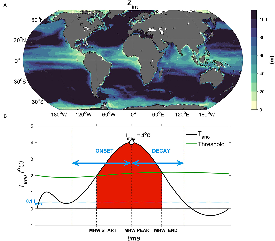
Figure 1. (A) Fixed depth (Zint) used for depth-integration of heat budget terms. Monthly climatology of mixed layer depth was derived from monthly outputs of density-based mixed layer depth at each pixel. The maximum from the monthly climatology were chosen as our fixed depth of integration. Note that Zint was capped at 110 m. (B) Schematics of the methodology used to identify MHW events, as well as its corresponding onset and decay period. According to Hobday et al. (2016) definition, a MHW occurs when the temperature anomaly (black) relative to an 11-day window climatology is above a threshold (green) defined as the 90th percentile based on the same climatology for a minimum of five consecutive days. Multiple metrics and characteristics are derived, including the maximum intensity (Imax) of the event (maximum temperature anomaly), which is defined as the MHW peak (Hobday et al., 2016). The onset (i.e., build-up of heat) and decay (i.e., dissipation of heat) were defined as periods when the temperature anomaly was above a value corresponding to 0.1 × Imax (blue). This way, the onset and decay periods include a larger portion of the temperature change associated with a MHW.

Note that the realization of a heat budget relative to a fixed depth has several advantages including a smaller computational effort, but also avoids numerical residuals that would be associated with the offline estimation of a daily varying MLD. In addition, this study focused on the most extreme events which are likely to last several months, across different seasons. Varying the depth of integration with the season was therefore impractical.

Marine Heatwave Identification

For the purpose of identifying the local physical drivers of MHWs via a heat budget analysis, events were identified during the entire 1984–2014 period, for all pixels separately. The Hobday et al. (2016) definition was adopted, using the 90th percentile threshold based on a 11-day window climatology. The three most extreme MHWs at each pixel (model grid) were selected based on values of cumulative intensity. Our analysis considers the three most extreme events to investigate common driving mechanisms. Importantly, our definition of “extreme” MHW differs from the category of “Extreme” defined by Hobday et al. (2018). Following the tropical cyclone scheme, they introduced four categories of MHWs based on their daily varying intensity (i.e., temperature anomaly). Here, a MHW is considered extreme based on its cumulative intensity relative to all other past events at the same pixel. The cumulative intensity metric allows a measure of the thermal anomaly stress (i.e., intensity) exerted by a MHW over its duration, which better captures the potential impact on marine ecosystems. This allows for the inclusion of all pixels in the analysis, as we consider extreme MHWs relative to a local measure of cumulative intensities. Although the cumulative intensity of an extreme MHW might be lower than the top three cumulative intensity values of an adjacent pixel, it remains extreme for local marine ecosystems. Note that this methodology does not guarantee spatial coherence of MHW events. For example, it is possible that the most extreme MHW in adjacent pixels can be associated with different distinct events, in different years and with varying drivers. This is illustrated by the important spatial noise of MHW peak dates in mid latitudes (Supplementary Figures 2A–C).

The anomalous temperature change associated with a MHW event (i.e., intensity) is defined relative to a climatological state. Start and end dates of an event indicate the moment when the temperature anomaly crossed the 90th percentile. Therefore, the period associated with the accumulation/dissipation of heat does not match the start and end date of an event. Onset and decay periods were calculated for each MHW, centered around the peak date, when the temperature anomaly was above 0.1 x maximum intensity (Figure 1A). The 0.1 factor increment allows for positive underlying trends that favor positive temperature anomalies toward the end of the model period. Note that this definition of onset and decay periods was chosen to provide an automated approach to better suit a global analysis and might not capture the exact temperature changes associated with the onset and decay of an individual MHW (Figure 1A).

Heat Budget

A heat budget was performed using OFAM3 outputs to quantify the contribution of local physical processes to the anomalous temperature change during each MHW onset and decay periods. The volume averaged temperature tendency equation is expressed as:

Where $\langle -\rangle =\frac{1}{V}\stackrel{V}{\int }dV$, V the volume defined by an area A and a depth h, u is the horizontal velocity vector, ∇_h is the horizontal gradient operator, w is the vertical velocity, Q is the net ASHF, ρ is the density of seawater (here we use ρ = 1,035 kg.m⁻³), C_pis the specific heat capacity of seawater and κ_h and κ_v are the horizontal and vertical diffusivity coefficients. Q (W.m⁻²) was calculated as the difference between the sum of net downward radiative and turbulent fluxes, and the penetrating shortwave radiation. Shortwave penetration was calculated using SeaWiFS monthly climatology of Kd-490, consistent with the methodology used in OFAM3 (Lee et al., 2005). Kd-490 values were first bi-linearly interpolated on the OFAM3 grid to account for their larger spatial resolution (0.25°). The term T therefore represents the total volume averaged temperature change, AdvH and AdvV the heat convergence due to horizontal and vertical advection, Q_HF the contribution from ASHF and Residual combines processes due to mixing that cannot be resolved by a diagnostic budget. Note that the Residual term also includes sub-daily variability and numerical errors.

The computation of horizontal and vertical advection was expanded at each face of the volume defined by individual model cells using the flux formulation:

However, this form becomes ambiguous if applied for the horizontal and vertical contributions separately, as mass conservation does not apply (Montgomery, 1974). We apply a similar approach to Lee et al. (2004) that removes the dependence on zero-temperature reference to accurately represent the heat advection contribution to the given volume. The calculation of horizontal and vertical advection is written as follows:

Where W, E, S, N, bot, top, represent the western, eastern, southern, northern, bottom and top face of the orthogonal volume V, and u and v are the zonal and meridional components of velocity. The temperature change due to total advection is calculated as the sum of AdvH and AdvV. Both terms were then integrated vertically (from Z_int to the surface) to represent the contribution of advective processes to upper ocean temperature changes.

MHWs are defined as events of anomalously high temperatures (Hobday et al., 2016). To isolate the contribution of each heat budget term to anomalies in upper layer temperature (by which we define a MHW), we calculate anomalies of each right-hand side term of Equation (1). This was done by subtracting the daily varying 11-day window mean to each term, consistent with the calculation of temperature climatology from Hobday et al. (2016). Results shown in this study include all terms of Equation (1) accumulated over the onset and decay periods of the three most extreme MHWs at each horizontal pixel.

Results

Drivers of Upper Ocean Extreme Marine Heatwaves

MHWs can be decomposed into an onset and decay phase, associated with an accumulation and dissipation of heat, respectively. In this section, we examine the physical mechanisms contributing to temperature changes during distinct phases of extreme events. Results from the heat budget analysis of the onset period of the three most extreme events in each pixel are shown in Figure 2. The anomalous total change in temperature (deltaT), which is a proxy for MHW maximum intensity, is high in western boundary current systems and their extensions (Figures 2A–C). This result for western boundary current systems is consistent for all three most extreme events. DeltaT is higher than 3°C in the Agulhas retroflection and then along a portion of the Antarctic Circumpolar Current (ACC) in the Indian Ocean. The largest deltaT is evident in the eastern equatorial Pacific for the strongest event, reaching 4–5°C, but decreases to <3°C for the second and third most intense events.

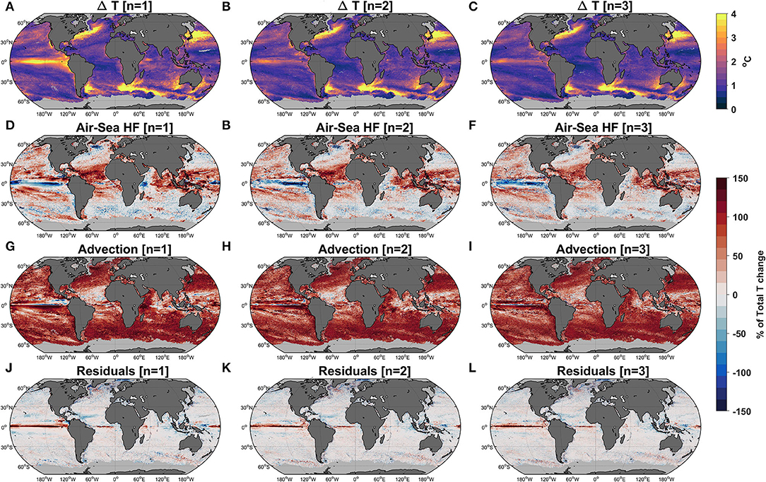
Figure 2. Heat budget results for the onset of the three strongest MHW events. (A–C) Total depth-averaged temperature anomaly change. The contribution from (D–F) total air-sea heat flux and (G–I) heat advection anomaly terms are shown as a percentage of the total temperature change. (J–L) The remaining temperature change that was not explained by either total air-sea heat flux nor advection are termed residuals. As temperature change is, by definition, positive during the onset period, positive/negative percentages indicate a warming/cooling contribution. Grid points where onset periods started before Jan-1st 1984 or with sea-ice contamination were excluded from the analysis (gray shading).

The contribution of Air-Sea Heat Fluxes (ASHF) is greater than horizontal advection in most of the tropics (Figure 2), heating the upper ocean to more than 50% of the MHW maximum. This excludes a narrow band along the equator and the western Indian Ocean, where ASHF has a cooling contribution during the onset period. ASHF contribution lessens in higher latitudes, acting against anomalous heat accumulation (i.e., cooling) in most subtropical regions. The cooling by ASHF is especially evident in western boundary current regions and their extensions, including the ACC. In contrast, the warming by heat advection is important in mid-high latitudes, explaining most of the temperature increase. Even in regions where advection plays a lesser role in driving temperature increases, such as in the tropics, its contribution is systematically positive and amplifies the strength of the MHW. The residual term (e.g., combining mixing and unresolved processes) contributes to <15% of deltaT for all three most extreme events across all ocean pixels. This result highlights that the onset of the most extreme events can be explained by the combination of anomalous surface heat flux and ocean heat advection. Nevertheless, the heat budget results in a large positive residual term along a narrow equatorial band in most of the Pacific and Atlantic Oceans, contributing to more than 100% of the warming observed during the onset period of all 3 strongest events. This large residual suggests that anomalous heat in this region may be due to processes such as horizontal and/or vertical mixing. In the tropical Pacific, the top 3 MHWs coincided with El Nino events of 97/98, 87 and 91/92, respectively (Supplementary Figure 2). These events are characterized by a deepening of the thermocline (Supplementary Figure 3), consistent with the large warming anomalies observed due to a decreased mixing (Figure 2).

The heat budget of the MHW decay periods, corresponding to the onset periods analyzed in Figure 2, is shown in Figure 3. Similar to onset periods, the ASHF term has a higher contribution to the decay of temperature anomalies through cooling in the tropics. In mid-high latitudes, heat advection remains the larger contributor to the decay of MHWs, explaining more than 50% of the cooling in most regions. However, the relative importance of advection in extra-tropical latitudes is reduced in favor of cooling from ASHFs. Indeed, 10–30% of the cooling during decay periods of MHWs is explained by a net ASHF from ocean to atmosphere. Note that close to the equator, especially in the tropical Pacific, surface ASHFs are either strongly contributing to the cooling (n = 1 & n = 2; Figures 3D,E) or neutral (n = 3; Figure 3F), while they are strongly opposing warming during onset periods (Figures 2D–F). The residual term for the decay period is negligible in most regions, except in the same narrow band around the equator and some regions in high latitudes (Figures 3J–L). Unlike during onset periods, the residual term during decay opposes the cooling tendency near the equator, suggesting that a decreased mixing acts to mitigate the decay of MHWs. In higher latitudes, the residual term has a positive contribution to cooling, locally explaining most of the decay of MHWs west of Cape Horn (120°W−55°S) or in parts of the northern Atlantic.

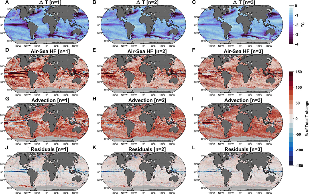
Figure 3. Same as Figure 2 for the decay period. As temperature change is, by definition, negative during the decay period, positive/negative percentages indicate a cooling/warming contribution. Grid points where decay periods ended after Dec-31st 2014, or contaminated by sea-ice, were excluded from the analysis (gray shading).

The spatial pattern and amplitude of the relative contribution of heat budget terms to warming/cooling during onset/decay periods is remarkably coherent for all three most extreme MHWs (Figures 2, 3). This suggests that the combinations of the heat budget terms presented represent mechanisms of the onset and decay of extreme events that are active globally. Figure 4 summarizes the main driver of these extreme MHWs, based on their relative contribution to total anomalous temperature change. Heat budget terms are defined as the dominant term if they explain more than two thirds of the total temperature change alone. Total advection is found to be the main driver of MHW onset in 72% of the global ocean (Figure 4A). In contrast, extreme MHW onsets are mostly driven by ASHF in only 11% of the global ocean, in regions concentrated in the tropics, especially in the northern tropical Atlantic Ocean and around the Indonesian Seas. The Residual term is the largest term for only 1% of pixels analyzed and dominates along a narrow equatorial band in the Atlantic and eastern Pacific Ocean. For the remaining 16% of the global ocean, there is no dominant term driving MHW onsets. In this case, heat accumulation is driven by a comparable contribution of ocean dynamic and atmospheric processes. Such regions are mostly located in the tropics at the edges of the regions where ASHF is the main driver of MHW onset.

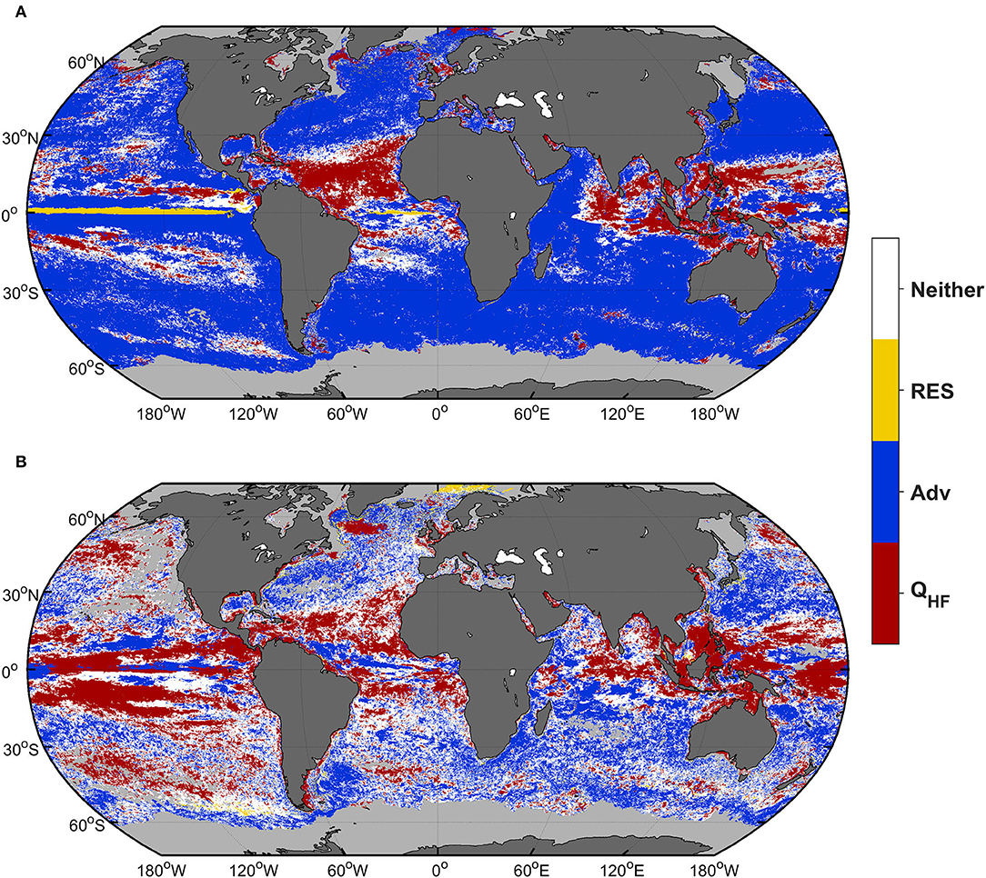
Figure 4. Main driver of most extreme MHWs (A) onset (n = 1–3) and (B) decay (n = 1–3). A heat budget term was defined as the main term when the average percent contribution to the total temperature change during onset or decay period across all three most extreme MHWs was larger than 66.6%. Note that only positive contribution to total temperature change was considered. In the case where no term's contribution was larger than 66.6%, the main driver was defined as “neither” (white), indicating that MHW onset or decay was driven by two or more terms. Net surface air-sea heat flux (red), total advection (blue) and the residual (yellow) term were considered [see Equation (1)].

Advection is remarkably less important in driving heat loss during MHW decay periods than for onset periods (Figure 4B). Heat divergence dominates MHW decay in only 31% of the global ocean. In contrast, the MHW decay is dominated by the ASHF term in 24% of the global ocean (compared to 11% during MHW onset), covering most of the northern tropical Atlantic, the eastern tropical Indian and western tropical Pacific Ocean. The lower importance of advection during the decay period is further demonstrated by the large increase in the number of pixels where there is no dominant term driving MHW decay. This is the case for 43% of pixels analyzed, with an enhanced shift in mid-high latitudes, where heat advection dominates the MHW onset period (Figure 4A). These results suggest that while ocean dynamics (i.e., advection) are dominant in driving extreme heat accumulation, the dissipation of upper ocean heat from the ocean to the lower atmosphere is critical in controlling the decay of MHWs in latitudes where the mixed layer is relatively deep (Figure 1B). Conversely, in the tropics, where the mixed layer is typically shallow (<50 m, Figure 1B), extreme MHW genesis and dissipation is mostly controlled by air-sea exchanges. Note that the residual term dominates the heat budget of extreme MHW decay in <2% of cases (Figure 4; compared with 1% for onset).

The decomposition of total heat advection into its horizontal and vertical components shows that vertical heat advection is negligible for the MHW development in most regions. The largest temperature changes during both phases of MHWs driven by advection occur in western boundary current systems and their extensions, as well as in the Leeuwin Current and the ACC south of the Indian Ocean (Figures 5A–C, 6A–C). The dominance of horizontal transport relative to its vertical component associated with these major currents indicates that vertical advection is negligible in the onset and decay of MHWs. Temperature changes during extreme MHWs in these regions are larger than 4°C and represent the largest temperature anomalies globally (Figures 2A–C). Two regions with large contributions from vertical advection are the equatorial eastern Pacific and western tropical Indian Ocean (Figure 5). The positive contribution of vertical advection to MHW onsets in these regions are associated with downwelling anomalies. Such anomalies can be attributed to planetary wave propagations associated with large climate modes of variability such as ENSO and the Indian Ocean Dipole (IOD), which are the primary modulators of MHW occurrences in the tropics (Holbrook et al., 2019). In contrast, during MHW decays, vertical advection is globally negligible compared to horizontal advection including in the eastern tropical Pacific and western Indian Ocean (Figure 6). It is only for the most extreme MHW event, in the eastern tropical Pacific, that vertical advective cooling dominates (Figure 6G). This particular event is associated with the 1997–98 El-Nino event (Supplementary Figure 2A), which transitioned into a La Nina event in 1998, driving enhanced upwelling and cooling of the upper tropical eastern Pacific Ocean (Picaut et al., 2002).

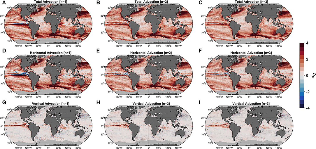
Figure 5. Decomposition of the heat advection term for the onset of the three strongest MHW events. (A–C) Total heat advection contribution to depth-averaged temperature anomaly change. Total heat advection was decomposed into its (D–F) horizontal component and (G–I) vertical component. Positive/negative values correspond to heat convergence/divergence. Grid points where onset periods started before Jan-1st 1984 or with sea-ice contamination were excluded from the analysis (gray shading).

Figure 6. The structure of the figure is the same as Figure 5 where the labeling is explained. Grid points where decay periods ended after Dec-31st 2014, or contaminated by sea-ice, were excluded from the analysis (gray shading).

Because we use a full radiation and turbulent heat flux budget, it is possible to examine the specific contributions of the individual surface heat fluxes to net ASHFs. For the MHW onsets the largest contributors to ASHF are mostly from anomalies of latent heat flux (Figure 7). This includes regions where ASHF is the main contributor of heat accumulation and are concentrated in the tropics (e.g., northern tropical Atlantic, eastern tropical Indian and western tropical Pacific; Figure 4A). Short wave radiation is the second highest contributor to ASHF in the tropics, despite a much smaller net contribution than latent heat flux (Figure 7). However, an anomalous decrease of shortwave radiation explains most of the negative contribution of ASHF to the onset of advective MHWs in the equatorial Pacific. This anomalous decrease is consistent with typical El-Nino conditions: increased upper ocean heat content in the eastern tropical Pacific increases convection and cloud formation and induces a decrease of short-wave radiation warming and increased evaporative (e.g., latent heat flux) cooling (Mayer et al., 2014). The cooling contribution of ASHF to MHW onset in higher latitudes is explained by increases in latent heat cooling (Figures 7G–I). The signal is most pronounced at western boundary current extensions and the ACC. Sensible heat flux cooling further contributed to reducing the overall heat convergence during MHW onsets in these regions. This suggests that the opposing latent and sensible heat flux cooling is a response to the high temperature anomalies being advected. Increased latent heat flux cooling also explains most of the ASHF contribution to upper ocean cooling during MHW decays (Figures 8G–I). In the tropics, the shortwave radiative cooling contribution dominates other heat flux terms in driving ASHF cooling and therefore MHW decays. This is particularly evident in the maritime continent region and the central equatorial Pacific (Figures 8D–F). Sensible heat flux cooling persists from MHW onset periods to decay periods and supports latent heat flux cooling in mid latitudes associated with western boundary current extensions and the ACC (Figures 8M–O).

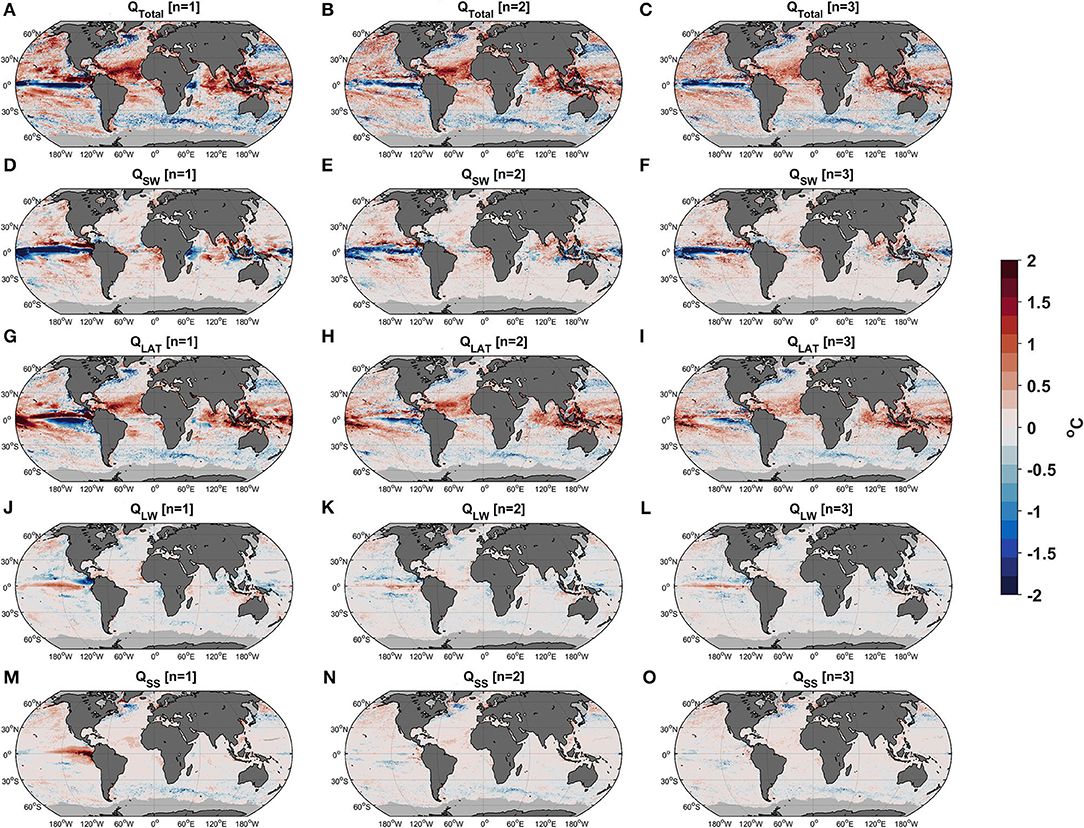
Figure 7. Decomposition of net air-sea heat flux contribution to the onset of the three strongest MHW events. (A–C) Net air-sea heat flux contribution to depth-averaged temperature anomaly change. Net air-sea heat flux was decomposed into (D–F) its shortwave radiation (G–I) latent heat flux (J–L) longwave radiation and (M–O) sensible heat flux components. Grid points where onset periods started before Jan-1st 1984 or with sea-ice contamination were excluded from the analysis (gray shading). Positive heat flux is a flux into the ocean, and in the case of latent heat it also means a gain of freshwater at the ocean surface.

Figure 8. The structure of the figure is the same as Figure 7 where the labeling is explained. Grid points where decay periods ended after Dec-31st 2014, or contaminated by sea-ice, were excluded from the analysis (gray shading).

Surface Signature of Extreme Upper Ocean Marine Heatwaves

A majority of MHW studies have focused on sea surface temperatures due to the larger number of observations and the availability of multiple satellite SST products, allowing for long-term gap free daily data. Despite recent efforts to increase our understanding of how surface MHWs relate to sub-surface MHWs (Schaeffer and Roughan, 2017; Elzahaby and Schaeffer, 2019; Elzahaby et al., 2021), there is little knowledge of their relationship on a global scale. OGCMs provide sub-surface data allowing the study of sub-surface MHWs and their comparison with surface events.

Figure 9 summarizes the sea surface signature of the three most extreme upper ocean MHWs. These strong events coincide almost systematically with at least one event at the surface (Figures 9A–C). This is the case in 97.2, 94.8, and 92.3% of pixels for the first, second and third most extreme upper ocean MHW, respectively. We note that the proportion of matching pixels is higher in the tropics compared to higher latitudes and decreased slightly with the rank of the upper ocean MHW. In a large number of pixels (Figures 9D–F), there is more than one surface MHW occurring during a single extreme upper ocean MHW. For example, 37.4% of the global ocean had two or more surface MHWs during the most extreme upper ocean event, decreasing to 27.2 and 21.7% for the second and third ranked upper ocean MHW.

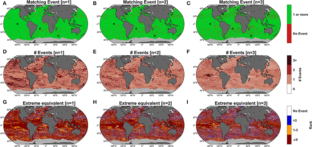
Figure 9. Surface signature of upper ocean 3 (n = 1–3, from left to right) most extreme MHWs. (A–C) Locations where the nth most extreme upper ocean MHW events coincided with a surface MHW event. Pixels where at least one surface MHW event period (e.g., start to end of MHW) intersected with the upper ocean MHW period were defined as matching (green). (D–F) Number of surface MHWs intersecting with the nth most extreme MHW event. Pixels where the nth most extreme upper ocean MHW did not coincide with any surface MHW was plotted in white. (G–I) Rank difference of cumulative intensity sum of surface MHWs coinciding with the nth most extreme upper ocean MHW, relative to all surface MHWs identified during the 1984-2014 period (Surface Extreme Equivalent). A value of 0 or less signifies that the surface signature MHW was at least as extreme. In contrast, a value of 1 signifies that the surface signature was 1 rank (relative to n) less extreme. Surface MHWs were identified according to the Hobday et al. (2016) definition. Grid points contaminated by sea-ice were excluded from the analysis (gray shading). The black boxes denote the location of pixels chosen in Supplementary Figure 3.

The sum of cumulative intensity of all surface MHWs occuring during an extreme upper-ocean MHW is ranked relative to the cumulative intensity of all surface MHWs identified during the 1984–2014 period (Surface Extreme Equivalent; SEE). This ranking value indicates how extreme is the surface response during the most extreme upper ocean MHWs. For example, a SEE value of 1 indicates that the surface signature is the most extreme when compared to all other surface MHWs. Figure 9 (bottom row) shows the difference of the SEE value with the rank of the upper ocean MHW it is compared against. Negative/positive differences signify that the surface signature is more/less extreme than the upper ocean. The most extreme upper ocean event translated into the most extreme surface signature in 65% of pixels. In an additional 23.6% of pixels, the surface signature is between the second and fourth most extreme heat event, leaving only 8.6% of pixels (excluding pixels where there is no surface event) where the surface signature ranks lower than fifth in terms of cumulative intensity. This result highlights the strong relationship between the upper ocean and the surface MHW state. For less extreme upper ocean MHWs, this relationship is still evident. SEE is within two units of the upper ocean MHW rank in 80 and 73% of cases for the second and third most extreme event, respectively. The correspondence between upper ocean and surface heat flux is much more consistent in tropical regions.

Discussion

Comparisons With Observed Events

Here, we perform the first global depth-integrated heat budget analysis applied to temperature variations during MHWs. Our results reveal that the most extreme upper ocean MHW onsets are due to anomalous convergence of heat driven by advection, except in tropical regions, where most MHWs are driven by anomalous heat fluxes into the ocean (Figure 5). In contrast, the decay of these MHWs is globally driven by a combination of anomalous heat divergence and ASHF cooling, both contributing equivalently to the total anomalous temperature change. Previous studies investigating the local physical drivers of major upper ocean MHWs support our results showinga dominance of oceanic advection driving heat convergence in extra-tropical regions. Both the western Australian summer 2011 (Benthuysen et al., 2014) and the summer 2016 Tasman Sea (Oliver et al., 2017). MHWs were generated by anomalous horizontal heat convergence that resulted from increased transport of the Leeuwin and East Australian Currents, respectively. In the East China Seas, recent major MHWs have been linked to a combination of heat convergence and anomalous ASHF into the ocean (Gao et al., 2020). In line with past results, we find that MHW onsets in the East China Seas are a combination of ASHF and advection (Figure 4). The spatial extent of MHWs dominated by ASHF is consistent with the location of past events. In 2015–2016, a reduction in upward ASHF was associated with severe warming in northern tropical Australia (Benthuysen et al., 2018).

In the literature, there has been a clear bias toward understanding how MHW temperature anomalies form, but only a few studies have investigated drivers of MHW decay. Heat dissipation was associated with increased ASHF cooling in most cases via an increase of latent heat cooling and/or upward (toward the atmosphere) sensible heat flux (Mayer et al., 2014; Kataoka et al., 2017; Sen Gupta et al., 2020). Our analysis supports the importance of ASHF in driving the decay of MHWs globally, including when and where MHWs are primarily generated by advection (e.g., compare Figure 2 with Figure 3 in mid-high latitudes). The conceptual diagram in Figure 10 summarizes phases of MHW events through the feedback processes responsible for the convergence and dissipation of heat. Increased incoming shortwave radiation and/or decreased latent heat loss usually control MHW onset generated by ASHF warming (Oliver et al., 2021). Variations of radiative and/or turbulent heat fluxes, which are typically driven by weather patterns (i.e., atmospheric highs, Rossby waves) initiate local increases in temperature. As the upper ocean heat accumulates, the ASHF warming is dampened by a latent heat loss feedback due to the excess heat available to evaporate moisture from the sea surface. During the peak of a MHW, warming and cooling processes balance each other and maintain temperature anomalies. During the decay phase, convection favorable weather patterns promote a shift in ASHF to cooling-favorable conditions. This results in a net loss of latent heat and sensible heat accentuated by an eventual decrease in incoming shortwave radiation due to cloud formation. In the case of an advective MHW, the same feedback mechanism occurs, as illustrated by the cooling contribution of latent heat flux during MHW onsets in extra-tropical regions (Figure 7). Heat convergence outweighs ASHF cooling until the peak of the MHW when the anomalous heat has dampened or reversed horizontal thermal gradients. This shift then initiates advective cooling, enhanced by the latent/sensible heat loss feedback, working simultaneously to promote the MHW decay.

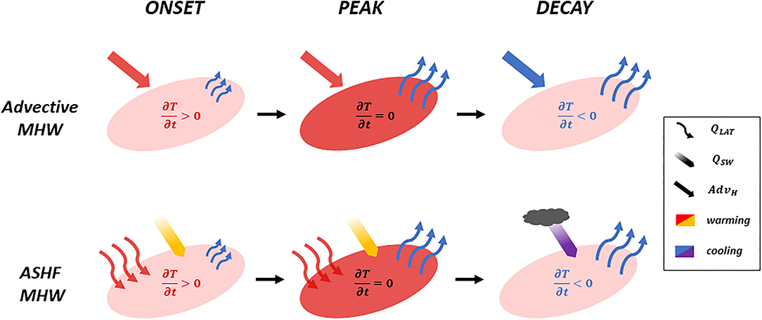
Figure 10. Mechanisms of upper ocean temperature feedback responses associated with an extreme advective and air-sea heat flux (ASHF) driven MHW during the onset, peak and decay periods.

It is important to highlight some of the caveats induced by the nature of this analysis. Results presented in this study are only representative of extreme MHWs, as we focused on the three most extreme events. Weaker MHWs have a weaker temperature anomaly signature and have a shorter lifespan than more extreme MHWs (Sen Gupta et al., 2020) and more likely to have more mixed contributions from the ASHF and advective terms. Local processes controlling heat variations over shorter time scales can differ regionally. This was illustrated by Li et al. (2020), who identified that only half of the events in the south-eastern waters of Australia were advection dominated, but that the proportion increased greatly for stronger events (in terms of cumulative intensity, Table 1). In addition, this analysis is not targeted to observed MHW drivers. The model used is free-running (but driven by realistic atmospheric forcing) and does not contain extensive data assimilation (only relaxation). This explains the lack of agreement between the model and observations in highly dynamic regions, where events are shorter, stochastic and greatly influenced by anticyclonic eddy propagation (Supplementary Figure 1). This type of MHW event is not well-resolved and is difficult to predict (Hallberg, 2013; Pilo et al., 2019; Hayashida et al., 2020). Driven by rising ocean surface temperatures (Frölicher et al., 2018; Darmaraki et al., 2019; Oliver, 2019; Marin et al., 2021) and the recent surge of scientific interest, most major MHW events studied occurred in the last few years. The OFAM3 run only covered the 1984–2014 period and consequently, some of the most recent events are missing from the analysis. Indeed, the impact of anthropogenic forcing on the global distrubution of MHW drivers is negeligeable given the absence of any significant trend (Supplementary Figure 4).

The identification of the onset and decay of MHWs was based on a subjective assessment of reasonable temperature threshold relative to MHW maximum intensity to accommodate for a global pixel-scale repeatability. Onset and decay periods might therefore differ significantly from other periods used for heat budget analysis in the past literature. Moreover, a strong event identified relative to a large box average might not be represented on pixel scale. For example, Chen et al. (2015) attributed the 2012 spring-summer MHW in the northwest Atlantic to anomalous ASHF while advection dampened the warming signal. While it was one of the most extreme events of the past decades on a large scale (Schlegel et al., 2021), it is not necessarily the case on a smaller scale considered here. Indeed, only coastal pixels and a small number of offshore pixels were associated with this extreme 2012 MHW (not shown). Results for a large proportion of these pixels were consistent with Chen et al. (2015), especially nearshore, where ASHF was the dominating term for MHW onsets (Figure 3).

Upper Ocean vs. Surface

Due to the definition of upper ocean MHWs, we expect that the driving mechanism for these will differ from the MHWs defined by SST. Sen Gupta et al. (2020) investigated local drivers of the most extreme MHWss derived from an observational SST product (NOAA OISST v2.0). Sen Gupta et al. found that in the sub-tropics, the most extreme SST MHWs were associated with a decrease in latent heat flux cooling and an increase in incoming shortwave radiation driven by blocking atmospheric highs. Air-sea heat flux may be a dominant forcing for the mixed layer temperature (and to some extent SST) variability. However, our definition of the upper ocean is the water column above the winter mixed layer depth, which includes the seasonal thermocline during the summer period. Within an increased surface layer thickness, the air-sea flux proportionally plays a lesser role in the MHW whereas advection can integrate to play a more major role. Anomalous heating due to air-sea heat flux increases stratification and is accompanied by a shoaling of the mixed layer depth, further enhancing temperature anomalies (Oliver et al., 2021). The resulting temperature increase is therefore restricted to a thinner surface layer, which explains the tendency of surface MHWs to be more responsive to changes in ASHF (Sparnocchia et al., 2006; Olita et al., 2007; Schlegel et al., 2021), increasing their frequency but decreasing their duration (Darmaraki et al., 2020). Indeed, this global study clearly shows that ASHF is the strongest driver of extreme MHW (Figure 3) in regions where the surface mixed layer is thinner (e.g., in the tropics, Figure 1). Importantly, monthly climatologies of MHW drivers within specific latitudinal bands did not show any significant seasonality (Supplementary Figure 4), suggesting that the sensitivity of the conclusions of our study to the season of occcurence of MHWs is limited.

Intensification of surface temperature responses to changes in ASHF also explains why upper ocean MHWs can coincide with multiple surface events (Figure 9). Atmospheric weather patterns have a relatively high frequency of variability and are more likely to dampen/enhance the surface warming signal during an upper ocean event. The increase of temperature variance can force surface temperatures below the MHW threshold for more than three consecutive days, which would create two distinct MHW events. This decoupling is more evident for the most extreme MHW event (Figure 9), as they are much longer (Supplementary Figure 2), increasing the probability of disruption of the continuity of the MHW surface disruption.

Nevertheless, there is high consistency between surface and upper ocean MHWs (Figures 9A–C). Our findings confirm that surface MHWs often extend well-below the surface. In fact, studies have shown that MHW intensity greatly increases with depth (Schaeffer and Roughan, 2017; Benthuysen et al., 2018; Hu et al., 2021). The generation of upper-ocean MHWs may contribute to SST MHW expressions which can be dampened/enhanced by surface fluxes. The sub-surface expression of the MHW can however remain for a much longer period of time and eventually resurface during well-mixed winter conditions (Scannell et al., 2020). By providing an implicit link between surface and subsurface MHWs, this work highlights the need of the MHW scientific community to consider the upper ocean in future MHW studies.

In part, this coherence can also be explained by our choice of selection of the most extreme MHWs. In the case where lower atmospheric processes oppose an advective MHW (e.g., upward ASHF), the depth-integrated event (upper ocean) would be less likely to be considered extreme. Our methodology choice should also favor events due to advection and ASHF acting in concert to enhance the extreme. In spite of this selection of the extremes, there are regions where two main terms of the heat budget give counter intuitive results and where particular terms are much stronger than the others. Following a local study by Schlegel et al. (2021), a further analysis of differences between extreme and average events can potentially reveal whether the type and spatial patterns of common MHW drivers differ from the most extreme events on a larger scale.

Conclusion

We have provided the first global analysis of the local processes controlling onset and decay of extreme MHWs using output from an OGCM. Horizontal upper ocean heat convergence is responsible for the onset of most MHWs. ASHF anomalous warming dominates the build-up of temperature anomalies in tropical regions where the upper ocean layer is shallower, mostly through a reduction in latent heat cooling or an increase in incoming shortwave radiation. While ASHF is the main driver of the decay of ASHF-driven MHWs, it also plays a crucial role in dissipating heat associated with advective MHWs. In this case, cooling is controlled by both heat divergence due to the dampening of thermal gradients and a latent heat loss feedback from excess upper ocean heat content. We also found that most upper ocean MHWs have a surface signature, although the amplitude of the surface signature is reduced in mid-high latitudes where the upper ocean layer is deeper. Capturing accurate long-term changes in MHWs using OGCM hindcasts has been shown to require realistic representation of external forcing induced by climate change (Frölicher et al., 2018; Bindoff et al., 2019; Darmaraki et al., 2019; Oliver et al., 2019; Hayashida et al., 2020; Marin et al., 2021). In addition, our work demonstrates that realistic simulation of MHW onset and decay demands that models and forcing accurately reproduce local atmospheric and ocean dynamics driven by internal variability processes. Key challenges include improving horizontal and vertical resolution as well as expanding ocean observing systems to support data assimilation approaches and improving the model's initial state (Bauer et al., 2015). This will ensure that extreme climatic events, including MHWs, will be the better represented and predicted by the future generation of models.

Data Availability Statement

The original contributions presented in the study are included in the article/Supplementary Material, further inquiries can be directed to the corresponding author.

Author Contributions

MM performed the analysis, most of the research design, and wrote the early version of the manuscript. MF, NB, and HP all helped to refine the research design, interpret the results, and participated in improving the manuscript. All authors contributed to the article and approved the submitted version.

Funding

MM and MF are partly supported by a CAS-CSIRO collaboration project on comparative studies of marine ecosystems between Australia and China. MM, HP, and NB acknowledge support from the Australian Research Centre for Excellence in Climate Extremes. HP and NB acknowledge funding from the Earth Systems and Climate Change and Climate Systems Hubs of the Australian Government's National Environmental Science Program and grant funding from the Australian Government as part of the Antarctic Science Collaboration Initiative Program.

Conflict of Interest

The authors declare that the research was conducted in the absence of any commercial or financial relationships that could be construed as a potential conflict of interest.

Publisher's Note

All claims expressed in this article are solely those of the authors and do not necessarily represent those of their affiliated organizations, or those of the publisher, the editors and the reviewers. Any product that may be evaluated in this article, or claim that may be made by its manufacturer, is not guaranteed or endorsed by the publisher.

Acknowledgments

This research was undertaken with the assistance of resources from the National Computational Infrastructure (NCI Australia), an NCRIS enabled capability supported by the Australian Government. The authors acknowledge NASA Goddard Space Flight Center, Ocean Ecology Laboratory, Ocean Biology Processing Group for providing the SeaWiFS ocean color data (https://oceancolor.gsfc.nasa.gov/data/10.5067/ORBVIEW-2/SEAWIFS/L2/OC/2018/).

Supplementary Material

The Supplementary Material for this article can be found online at: https://www.frontiersin.org/articles/10.3389/fclim.2022.788390/full#supplementary-material

References

Babcock, R. C., Bustamante, R. H., Fulton, E. A., Fulton, D. J., Haywood, M. D. E., Hobday, A. J., et al. (2019). Severe continental-scale impacts of climate change are happening now: extreme climate events impact marine habitat forming communities along 45% of Australia's coast. Front. Mar. Sci. 6, 411. doi: 10.3389/fmars.2019.00411
Bauer, P., Thorpe, A., and Brunet, G. (2015). The quiet revolution of numerical weather prediction. Nature 525, 47–55. doi: 10.1038/nature14956
Benthuysen, J. A., Feng, M., and Zhong, L. (2014). Spatial patterns of warming off Western Australia during the 2011 Ningaloo Niño: quantifying impacts of remote and local forcing. Cont. Shelf Res. 91, 232–246. doi: 10.1016/j.csr.2014.09.014
Benthuysen, J. A., Oliver, E. C. J., Feng, M., and Marshall, A. G. (2018). Extreme marine warming across tropical Australia during austral summer 2015-2016. J. Geophys. Res. Oceans 123, 1301–26. doi: 10.1002/2017JC013326
Bindoff, N. L., Cheung, W. W. L., Kairo, J. G., Arístegui, J., Guinder, V. A., Hallberg, R., et al. (2019). “Changing ocean, marine ecosystems, and dependent communities,” in IPCC Special Report on the Ocean and Cryosphere in a Changing Climate, eds H.-O. Pörtner, D. C. Roberts, V. Masson-Delmotte, P. Zhai, M. Tignor, E. Poloczanska, et al., 450–545.
Caputi, N., Kangas, M., Chandrapavan, A., Hart, A., Feng, M., Marin, M., et al. (2019). Factors affecting the recovery of invertebrate stocks from the 2011 Western Australian extreme marine heatwave. Front. Mar. Sci. 6, 484. doi: 10.3389/fmars.2019.00484
Chen, K., Gawarkiewicz, G., Kwon, Y.-O., and Zhang, W. G. (2015). The role of atmospheric forcing versus ocean advection during the extreme warming of the Northeast U.S. continental shelf in 2012. J. Geophys. Res. Oceans 120, 4324–4339. doi: 10.1002/2014JC010547
Collins, M., Sutherland, M., Bouwer, L., Cheong, S.-M., Fröliche, T., Combes, H. J., et al. (2019). “Extremes, abrupt changes and managing risk,” in IPCC Special Report on the Ocean and Cryosphere in a Changing Climate, eds H.-O. Pörtner, D.C. Roberts, V. Masson-Delmotte, P. Zhai, M. Tignor, E. Poloczanska.
Darmaraki, S., Somot, S., Sevault, F., Nabat, P., Cabos Narvaez, W. D., Cavicchia, L., et al. (2019). Future evolution of marine heatwaves in the mediterranean sea. Clim. Dyn. 53, 1371–92. doi: 10.1007/s00382-019-04661-z
Darmaraki, S., Somot, S., Waldman, R., Sevault, F., Nabat, P., and Oliver, E. (2020). Mediterranean Marine Heatwaves: On the Comparison of the Physical Drivers Behind the 2003 and 2015 events. EGU General Assembly 2020, Online, 4–8 May 2020, EGU2020–12104. doi: 10.5194/egusphere-egu2020-12104
Dee, D. P., Uppala, S. M., Simmons, A. J., Berrisford, P., Poli, P., Kobayashi, S., et al. (2011). The ERA-interim reanalysis: configuration and performance of the data assimilation system. Q. J. R. Meteorol. Soc. 137, 553–597. doi: 10.1002/qj.828
Elzahaby, Y., and Schaeffer, A. (2019). Observational insight into the subsurface anomalies of marine heatwaves. Front. Mar. Sci. 6, 745. doi: 10.3389/fmars.2019.00745
Elzahaby, Y., Schaeffer, A., Roughan, M., and Delaux, S. (2021). Oceanic circulation drives the deepest and longest marine heatwaves in the East Australian current system. Geophys. Res. Lett. 48, e2021GL094785. doi: 10.1029/2021GL094785
Feng, M., McPhaden, M. J., Xie, S.-P., and Hafner, J. (2013). La Niña forces unprecedented Leeuwin current warming in 2011. Sci. Rep. 3, 1277. doi: 10.1038/srep01277
Feng, M., Zhang, X., Oke, P., Monselesan, D., Chamberlain, M., Matear, R., et al. (2016). Invigorating ocean boundary current systems around Australia during 1979-2014: as simulated in a near-global eddy-resolving ocean model. J. Geophys. Res. Oceans 121, 3395–3408. doi: 10.1002/2016JC011842
Frölicher, T. L., Fischer, E. M., and Gruber, N. (2018). Marine heatwaves under global warming. Nature 560, 360–364. doi: 10.1038/s41586-018-0383-9
Gao, G., Marin, M., Feng, M., Yin, B., Yang, D., Feng, X., et al. (2020). Drivers of marine heatwaves in the East China sea and the south yellow sea in three consecutive summers during 2016–2018. J. Geophys. Res. Oceans 125, e2020JC016518. doi: 10.1029/2020JC016518
Garrabou, J., Coma, R., Bensoussan, N., Bally, M., Chevaldonne, P., Cigliano, M., et al. (2009). Mass mortality in Northwestern Mediterranean rocky benthic communities: effects of the 2003 heat wave. Glob. Chang. Biol. 15, 1090–1103. doi: 10.1111/j.1365-2486.2008.01823.x
Griffies, S., Harrison, M., C Pacanowski, R., and Rosati, A. (2004). A Technical Guide to MOM4. GFDL Ocean Group Technical Report NO. 5. Available online at: http://www.gfdl.noaa.gov (accessed April 4, 2021).
Griffies, S. M., and Hallberg, R. W. (2000). Biharmonic friction with a smagorinsky-like viscosity for use in large-scale eddy-permitting ocean models. Monthly Weather Rev. 128, 2935–2946. doi: 10.1175/1520-0493(2000)128<2935:BFWASL>2.0.CO;2
Hallberg, R.. (2013). Using a resolution function to regulate parameterizations of oceanic mesoscale eddy effects. Ocean Model. 72, 92–103. doi: 10.1016/j.ocemod.2013.08.007
Hayashida, H., Matear, R. J., Strutton, P. G., and Zhang, X. (2020). Insights into projected changes in marine heatwaves from a high-resolution ocean circulation model. Nat. Commun. 11, 1–9. doi: 10.1038/s41467-020-18241-x
Hobday, A. J., Alexander, L. V., Perkins, S. E., Smale, D. A., Straub, S. C., Oliver, E. C. J., Benthuysen, J. A., et al. (2016). A hierarchical approach to defining marine heatwaves. Prog. Oceanogr. 141, 227–238. doi: 10.1016/j.pocean.2015.12.014
Hobday, A. J., Oliver, E. C. J., Moore, P. J., Wernberg, T., and Smale, D. A. (2018). Categorizing and naming marine heatwaves. Oceanography 31, 162–173. doi: 10.5670/oceanog.2018.205
Holbrook, N. J., Scannell, H. A., Sen Gupta, A., Benthuysen, J. A., Feng, M., Oliver, E. C. J., et al. (2019). A global assessment of marine heatwaves and their drivers. Nat. Commun. 10, 1–13. doi: 10.1038/s41467-019-10206-z
Holbrook, N. J., Sen Gupta, A., Oliver, E. C. J., Hobday, A. J., Benthuysen, J. A., Scannell, H. A., et al. (2020). Keeping pace with marine heatwaves. Nat. Rev. Earth Environ. 1, 482–493. doi: 10.1038/s43017-020-0068-4
Hu, S., Li, S., Zhang, Y., Guan, C., Du, Y., Feng, M., et al. (2021). Observed strong subsurface marine heatwaves in the tropical western Pacific Ocean. Environ. Res. Lett. 16, 104024. doi: 10.1088/1748-9326/ac26f2
Kataoka, T., Tozuka, T., and Yamagata, T. (2017). Generation and decay mechanisms of Ningaloo Niño/Niña. J. Geophys. Res. Oceans 122, 8913–8932. doi: 10.1002/2017JC012966
Large, W. G., McWilliams, J. C., and Doney, S. C. (1994). Oceanic vertical mixing: A review and a model with a nonlocal boundary layer parameterization. Rev. Geophys. 32, 363–403. doi: 10.1029/94RG01872
Large, W. G., and Yeager, S. (2004). Diurnal to Decadal Global Forcing for Ocean and Sea-Ice Models: The Data Sets And Flux Climatologies (No. NCAR/TN-460+STR). University Corporation for Atmospheric Research. doi: 10.5065/D6KK98
Lee, T., Fukumori, I., and Tang, B. (2004). Temperature advection: internal versus external processes. J. Phys. Oceanogr. 34, 1936–1944. doi: 10.1175/1520-0485(2004)034<1936:TAIVEP>2.0.CO;2
Lee, Z.-P., Darecki, M., Carder, K. L., Davis, C. O., Stramski, D., and Rhea, W. J. (2005). Diffuse attenuation coefficient of downwelling irradiance: an evaluation of remote sensing methods. J. Geophys. Res. Oceans 110. doi: 10.1029/2004JC002573
Li, Z., Holbrook, N. J., Zhang, X., Oliver, E. C. J., and Cougnon, E. A. (2020). Remote forcing of tasman sea marine heatwaves. J. Clim. 33, 5337–5354. doi: 10.1175/JCLI-D-19-0641.1
Marin, M., Feng, M., Phillips, H. E., and Bindoff, N. L. (2021). A global, multi-product analysis of coastal marine heatwaves: distribution, characteristics and long-term trends. J. Geophys. Res. Oceans 126, e2020JC016708. doi: 10.1029/2020JC016708
Mayer, M., Haimberger, L., and Balmaseda, M. A. (2014). On the energy exchange between tropical ocean basins related to ENSO. J. Clim. 27, 6393–6403. doi: 10.1175/JCLI-D-14-00123.1
Mills, K. E., Pershing, A. J., Brown, C. J., Chen, Y., Chiang, F.-S., Holland, D. S., et al. (2013). Fisheries management in a changing climate. Oceanography 26, 191–195. doi: 10.5670/oceanog.2013.27
Montgomery, R. B.. (1974). Comments on “seasonal variability of the Florida Current,” by Niiler and Richardson. J. Mar. Res. 32, 533–535.
Oke, P. R., Griffin, D. A., Schiller, A., Matear, R. J., Fiedler, R., Mansbridge, J., et al. (2013). Evaluation of a near-global eddy-resolving ocean model. Geosci. Model Dev. 6, 591–615. doi: 10.5194/gmd-6-591-2013
Olita, A., Sorgente, R., Natale, S., Gaberšek, S., Ribotti, A., Bonanno, A., et al. (2007). Effects of the 2003 European heatwave on the Central Mediterranean Sea: surface fluxes and the dynamical response. Ocean Sci. 3, 273–289. doi: 10.5194/osd-3-85-2006
Oliver, E. C. J.. (2019). Mean warming not variability drives marine heatwave trends. Clim. Dyn. 53, 1653–59. doi: 10.1007/s00382-019-04707-2
Oliver, E. C. J., Benthuysen, J. A., Bindoff, N. L., Hobday, A. J., Holbrook, N. J., Mundy, C. N., et al. (2017). The unprecedented 2015/16 Tasman Sea marine heatwave. Nat. Commun. 8, 16101. doi: 10.1038/ncomms16101
Oliver, E. C. J., Benthuysen, J. A., Darmaraki, S., Donat, M. G., Hobday, A. J., Holbrook, N. J., et al. (2021). Marine heatwaves. Ann. Rev. Mar. Sci. 13, 313–342. doi: 10.1146/annurev-marine-032720-095144
Oliver, E. C. J., Burrows, M., Donat, M., Gupta, A., Alexander, L., Perkins-Kirkpatrick, S., et al. (2019). Projected marine heatwaves in the 21st century and the potential for ecological impact. Front. Mar. Sci. 6, 734. doi: 10.3389/fmars.2019.00734
Oliver, E. C. J., Donat, M. G., Burrows, M. T., Moore, P. J., Smale, D. A., Alexander, L. V., et al. (2018). Longer and more frequent marine heatwaves over the past century. Nat. Commun. 9. doi: 10.1038/s41467-018-03732-9
Picaut, J., Hackert, E., Busalacchi, A. J., Murtugudde, R., and Lagerloef, G. S. E. (2002). Mechanisms of the 1997–1998 El Niño–La Niña, as inferred from space-based observations. J. Geophys. Res. Oceans 107, 5–18. doi: 10.1029/2001JC000850
Pilo, G. S., Holbrook, N. J., Kiss, A. E., and Hogg, A. M. C. (2019). Sensitivity of marine heatwave metrics to ocean model resolution. Geophys. Res. Lett. 46, 14604–14612. doi: 10.1029/2019GL084928
Ridgway, K. R., Dunn, J. R., and Wilkin, J. L. (2002). Ocean interpolation by four-dimensional weighted least squares? Application to the waters around Australasia. J. Atmos. Ocean. Technol. 19, 1357–1375. doi: 10.1175/1520-0426(2002)019<1357:OIBFDW>2.0.CO;2
Santoso, A., Mcphaden, M. J., and Cai, W. (2017). The defining characteristics of ENSO extremes and the strong 2015/2016 El Niño. Rev. Geophys. 55, 1079–1129. doi: 10.1002/2017RG000560
Scannell, H. A., Johnson, G. C., Thompson, L., Lyman, J. M., and Riser, S. C. (2020). Subsurface evolution and persistence of marine heatwaves in the Northeast Pacific. Geophys. Res. Lett. 47, e2020GL090548. doi: 10.1029/2020GL090548
Schaeffer, A., and Roughan, M. (2017). Subsurface intensification of marine heatwaves off southeastern Australia: the role of stratification and local winds. Geophys. Res. Lett. 44, 5025–5033. doi: 10.1002/2017GL073714
Schlegel, R. W., Oliver, E. C. J., and Chen, K. (2021). Drivers of marine heatwaves in the Northwest Atlantic: the role of air–sea interaction during onset and decline. Front. Mar. Sci. 8, 217. doi: 10.3389/fmars.2021.627970
Sen Gupta, A., Thomsen, M., Benthuysen, J. A., Hobday, A. J., Oliver, E., Alexander, L. V., Burrows, M. T., et al. (2020). Drivers and impacts of the most extreme marine heatwaves events. Sci. Rep. 10, 19359. doi: 10.1038/s41598-020-75445-3
Smale, D. A., Wernberg, T., Oliver, E. C. J., Thomsen, M., Harvey, B. P., Straub, S. C., et al. (2019). Marine heatwaves threaten global biodiversity and the provision of ecosystem services. Nat. Clim. Change. 9, 306–12. doi: 10.1038/s41558-019-0412-1
Sparnocchia, S., Schiano, M. E., Picco, P., Bozzano, R., and Cappelletti, A. (2006). The anomalous warming of summer 2003 in the surface layer of the Central Ligurian Sea (Western Mediterranean). Ann. Geophys. 24, 443–452. doi: 10.5194/angeo-24-443-2006
Keywords: extreme marine heatwave, upper ocean, marine heatwave phases, physical drivers, heat advection, air-sea heat flux, global model
Citation: Marin M, Feng M, Bindoff NL and Phillips HE (2022) Local Drivers of Extreme Upper Ocean Marine Heatwaves Assessed Using a Global Ocean Circulation Model. Front. Clim. 4:788390. doi: 10.3389/fclim.2022.788390
Received: 02 October 2021; Accepted: 11 April 2022;
Published: 03 May 2022.
Edited by:
Svenja Ryan, Woods Hole Oceanographic Institution, United StatesReviewed by:
Robert William Schlegel, Institut de la Mer de Villefranche (IMEV), FranceSofia Darmaraki, Dalhousie University, Canada
Copyright © 2022 Marin, Feng, Bindoff and Phillips. This is an open-access article distributed under the terms of the Creative Commons Attribution License (CC BY). The use, distribution or reproduction in other forums is permitted, provided the original author(s) and the copyright owner(s) are credited and that the original publication in this journal is cited, in accordance with accepted academic practice. No use, distribution or reproduction is permitted which does not comply with these terms.
*Correspondence: Maxime Marin, maxime.marin@riskfrontiers.com