Nonlinear gas path analysis

Aeroengine nonlinear condition monitoring model can be expressed as the following nonlinear equations.

The components of the health parameter vector θ in the above equations are generally defined by the ratio of the performance parameters of the degraded or malfunctioning engine components to those of the clean engine components, and in the form of

In the numerical calculation of health parameter estimation, Equation 2 can be linearized at the currently estimated value of the health parameters θ^.

where the Jacobian matrix

Equation 4 can be written in residual form as

where the estimated measurement residual (in relative form)

and the estimated health parameter residual

Then in the kth iterative calculation, we have

Parameter selection

Identifiability analysis

When Equation 15 is full column rank, the health parameter corresponding to each column is identifiable. In this paper, the singular value decomposition method is used to obtain the rank of the matrix. Then the matrix in Equation 15 can be decomposed as

(16)

S(t)=U(t)Σ(t)VT(t)

The diagonal elements of Σ(t) are the singular values of S(t) in descending order, while the number of non-zero singular values is the rank. Each column of the unitary matrix V(t) represents one identifiable direction in the health parameter space under the current measurement settings, and the corresponding singular value indicates its degree of identifiability. The larger the singular value is, the greater the degree of stretching on the corresponding direction will be when transforming from the health parameter space to the measurement space, and then the easier to identify small changes of the health parameters. The above-mentioned health parameter space can be represented by a hyper-ellipsoid in a dimension equal to the number of health parameters. The singular vector and the reciprocal of the singular value correspond to the direction and relative length of the hyper-ellipsoid axis, respectively. A two-dimensional health parameter space is schematically illustrated in Figure 1.

Figure 1.

Two-dimensional health parameter identification space.

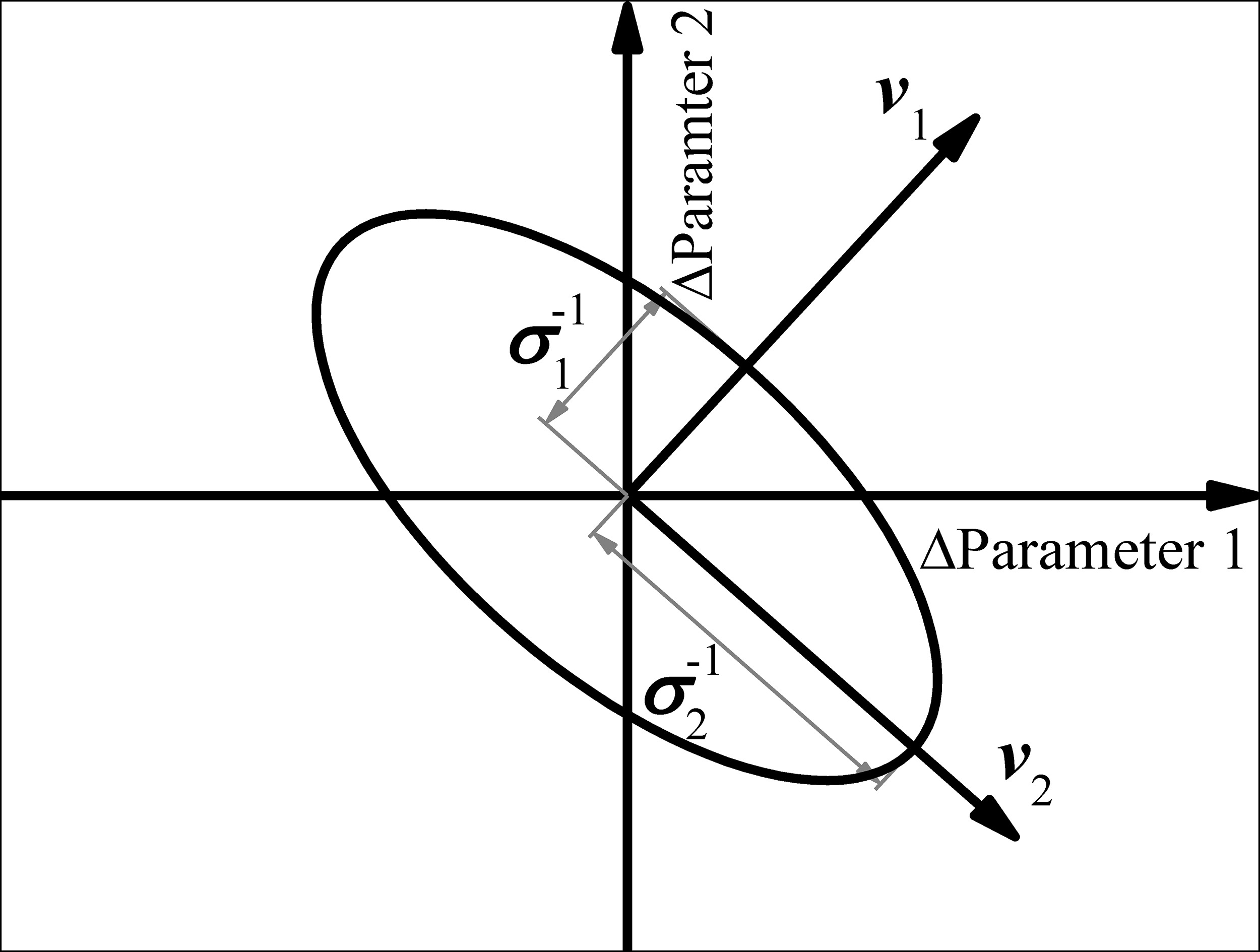
It is obvious that the longest axis of the hyper-ellipsoid determines the maximum span of the health parameter space, which corresponds to the upper bound of system uncertainty. Therefore, the smallest singular value σ_min(t) can be used to measure system identifiability.

The engine model

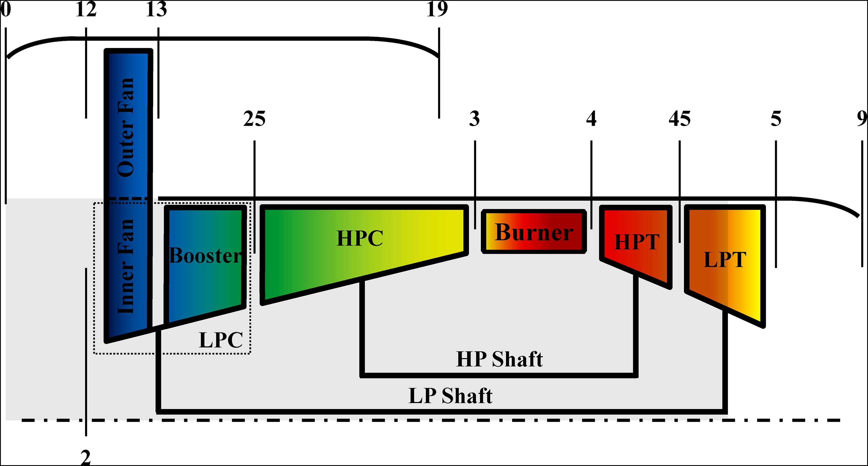
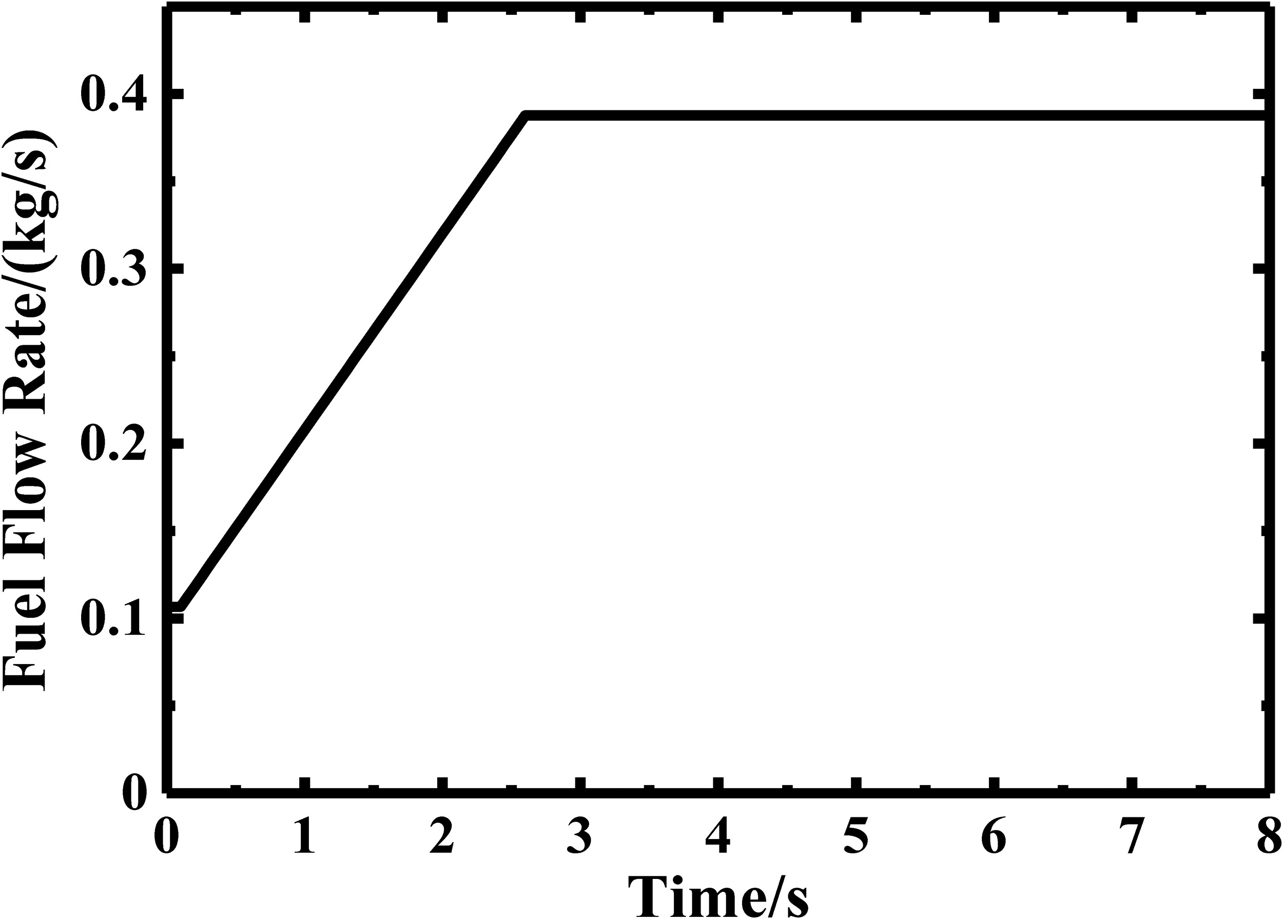
The engine model used for parameter selection is a separated flow turbofan engine. Figure 2 depicts the stations where outputs are simulated. A slam acceleration process using the fuel schedule shown in Figure 3 is chosen for the analysis.

Figure 2.

Schematic diagram of the simulated separated flow turbofan engine.

Figure 3.

Fuel schedule.

Measurement selection

Supposing there is instrumental redundancy. The candidate measurements, the health parameters to be estimated and their implanted deviations are listed in Table 1 (subscripts are described in Figure 1), where Γ and η represent the corrected flow rate and efficiency of the corresponding component. Sensor dynamics and noise are ignored for simplicity in this study.

To estimate all health parameters listed in Table 1, simultaneously, and avoid unnecessary instrument installation, we need to select 10 measurements among the 12 candidates in a way that is most conducive to engine health status estimation. There will be two ways involved in this paper for measurement selection: one is sensitivity analysis-based, and the other is identifiability analysis-based.

Health parameter selection

Supposing the number of measurements is limited. A typical 7 gas path measurements set is listed in Table 6.

It is not possible to estimate all the health parameters shown in Table 1 simultaneously using the measurement set given in Table 6, obviously. Therefore, we have to select the health parameter combinations that can be better identified. The health parameter selection problem considering here has the following features:

Results show that the maximum number of identifiable health parameters at t = 1 s is 7, and there are 10 feasible combinations, among which combination 3 has the highest identifiability (σmin) and a comparatively lower estimation error, but combination 1 has the least identifiability and estimation accuracy. Thereby we can put the health parameter combination with the highest identifiability at each sampling point into one best identifiability matrix as shown in Figure 4. The order of the health parameters in Figure 4 are consistent with Table 1. Colour blue and white represent “include” and “not include”, respectively.

Figure 4.

Health parameter best identifiability matrix.

It also shows that there are slightly differences of the maximum number of identifiable health parameters at different sampling points, that is, 7 for the majority of the sampling points except 6 at t = 1.7 s and t = 1.8 s.

Smearing effect analysis

Considering the identifiability of the engine health status on a component level by the measurement set shown in Table 6. According to the health parameters listed in Table 1, the health status of each main gas path component is described by two health parameters. So the maximum number of components that can be analysed simultaneously by the measurement set shown in Table 6 is 3 at each sampling point. Therefore, theoretically, the number of identifiable component combinations is C51+C52+C53=25.

By constructing the subsystem matrix of the 25 component combinations at a certain sampling point and calculating their rank, we can obtain the identifiability of these subsystems. The results are shown in Figure 5. The left part of Figure 5 shows the component combinations, with colour black and white represent “include” and “not include”, respectively. The right part of Figure 5 shows the identifiability of the corresponding component combination, with colour blue and white represent “identifiable” and “unidentifiable”, respectively.

Figure 5.

Component identifiability matrix.

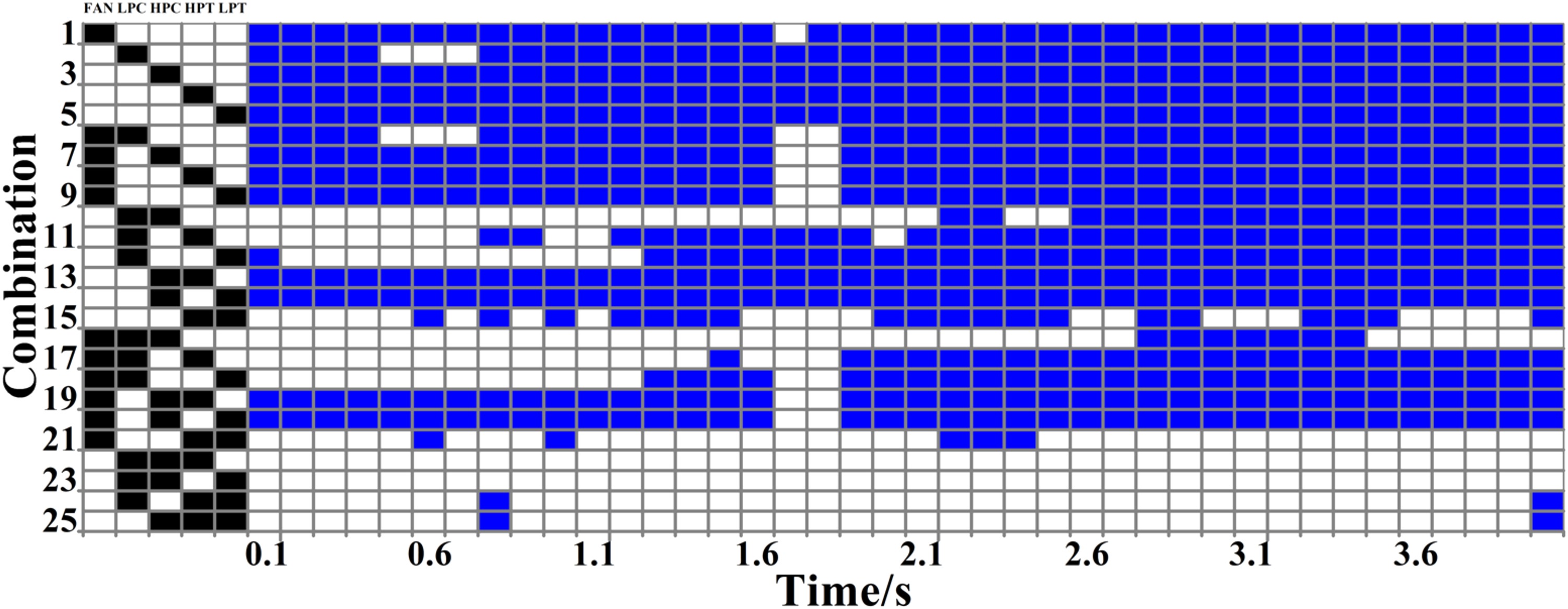
Figure 5 shows that the identifiability of the component combinations vary with sampling time as well as the number of components. In general, an increase in the number of components leads to a decrease in identifiability.

Take combination 10 and combination 15 as examples, the estimation results of these two combinations are shown in Figure 6. The number of combinations and sampling points are consistent with Figure 5, and the colour green, yellow, and red represent “converged with high precision”, “converged with low precision” and “diverged”, respectively.

Figure 6.

Estimation results of combination 10 and 15.

Combining the results in Figures 5 and 6, unsatisfactory estimation result only occurs when the corresponding component combination is unidentifiable. Take the results of combination 10 at t = 0.9 s and combination 15 at t = 0.1 s as examples (Figure 7).

Figure 7.

Estimation results of combination 10 at t = 0.9 s (left) and combination 15 at t = 0.1 s (right).

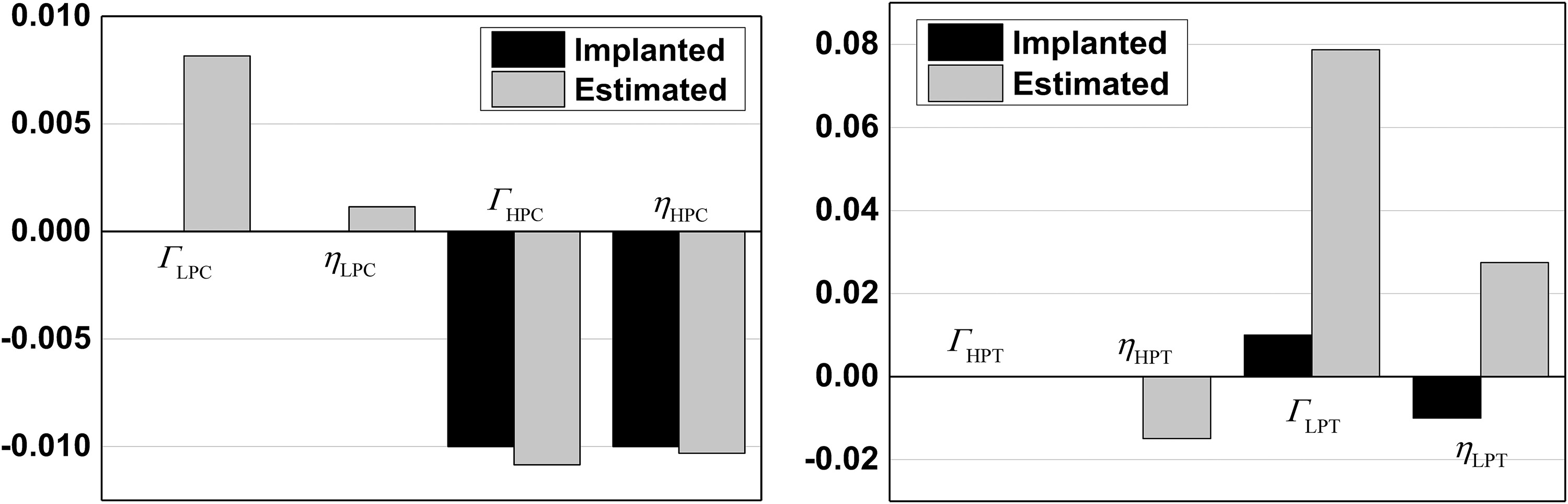
It is shown that there are large deviations in both cases, which means “smearing effect” occurs. Aretakis et al. (2002) and Mathioudakis et al. (2004) firstly pointed out this phenomenon in fault diagnosis, and they also provided a solution for this problem, that is, addition of measured quantities between the corresponding components. Based on the above results, it can be concluded that “smearing effect” is caused by the measurement set as well as the engine nonlinearity at a certain operating point, which means only when the combination of these two factors leads to a singular system, may this phenomenon occur. From the perspective of system identification, “smearing effect” means an increase in system uncertainty.

Subscript