
Online approximative SPARQL query processing for COUNT-DISTINCT queries with web preemption
Abstract
Getting complete results when processing aggregate queries on public SPARQL endpoints is challenging, mainly due to the application of quotas. Although Web preemption supports processing of aggregate queries online, on preemptable SPARQL servers, data transfer is still very large when processing count-distinct aggregate queries. In this paper, it is shown that count-distinct aggregate queries can be approximated with low data transfer by extending the partial aggregation operator with HyperLogLog++ sketches. Experimental results demonstrate that the proposed approach outperforms existing approaches by orders of magnitude in terms of the amount of data transferred.
1.Introduction
Context and motivation: Processing SPARQL aggregate queries on public SPARQL endpoints is challenging, mainly due to the fair-use policies of public endpoints that stop queries before termination [8,19]. For instance, a SPARQL query that computes the number of distinct objects per class, for all available classes, cannot be executed online on Wikidata or DBPedia. On both SPARQL endpoints, the query hits the quotas. Consequently, no results are delivered.
Related works: A common workaround for computing such queries relies on dataset dumps, but re-ingesting large dumps is very costly and time-consuming. Approximate Query Processing is a well-known approach for computing aggregations and can be updated to support fair-use policies [19], but requires to accept a trade-off between accuracy and response time. Restricted SPARQL servers such as TPF [23], Web preemption [14] or SmartKG [2] ensure termination of a restricted set of SPARQL operations, while preserving the responsiveness of the restricted server. Unfortunately, aggregate functions are not supported by the restricted SPARQL servers. Processing aggregate queries requires materializing the query mappings on the client-side before computing aggregates locally. Even if the processing is guaranteed to terminate, the size of the data transfer may be prohibitive.
In a previous work [7], we demonstrated that a partial aggregation operator is preemptable. Computing partial aggregations on a preemptable server drastically reduces data transfer for most aggregate queries, while ensuring complete results. However, count-distinct aggregate queries still generate a large data transfer, even with a partial aggregation operator. Computing the exact cardinality of a multiset requires a data transfer proportional to the size of the multiset, which is impractical for very large datasets.
Approach and Contributions: To improve the evaluation of count-distinct aggregate queries, the approach proposed in [7] is extended with HyperLogLog++ sketches. HyperLogLog++ is a probabilistic algorithm that can estimate the cardinality of large sets with a small amount of memory and strong guarantees on the error rate. As HLL++ supports the decomposability property of aggregate functions, it can be integrated into the partial aggregations framework promoted in [7]. Compared to related Approximated Query Approaches [19], this approach ensures to find all
– An extension of the partial aggregation operator presented in [7]. This extension allows estimating the result of a count-distinct query with a bounded error rate.
– Additional experimental results that compare the performance of the extended operator and the previous operator [7]. Experimental results demonstrate that relying on estimates does not improve the execution time, but significantly reduces the data transfer for count-distinct queries, and in the general case, show that the proposed approach outperforms existing approaches used for processing aggregate queries.
The remainder of this paper is structured as follows. Section 2 summarizes related works. Section 3 introduces SPARQL aggregate queries and the Web preemption model. Section 4 presents the approach for processing aggregate queries using a preemptive SPARQL server. Section 5 introduces HyperLogLog++ and its integration in the partial aggregation operator. Section 6 presents the different algorithms used to implement the proposed approach. Section 7 presents our experimental results. Section 8 discusses the limitations of the current proposal. Finally, conclusions and future work are outlined in Section 9.
2.Related works
Aggregate queries on public SPARQL endpoints Public endpoints such as DBPedia or Wikidata support any SPARQL aggregate queries. However, such queries are often long-running queries that require a lot of CPU and memory resources to terminate. To ensure stable and responsive services to the user community, public SPARQL endpoints set up quotas on the maximum number of results returned, execution time, and arrival rate. Consequently, many aggregate queries cannot be executed online, simply because they reach the quotas of the fair-use policies [3,14,19].
Use of dumps A common workaround for quota limitations relies on dumps of datasets. Datasets dumps have to be first re-ingested on local resources before executing aggregate queries [1,16]. As datasets become bigger and bigger, re-ingesting large datasets is very costly, time-consuming, and raises freshness issues. Re-ingesting data dumps can be profitable only if a high number of aggregate queries have to be executed. The purpose of this paper is to process aggregate queries online, i.e. without moving the data.
Decomposition of queries Another well-known approach to overcome quotas is to decompose a query into smaller subqueries that can be evaluated under quotas. Query results are then recombined on the client-side [3]. Such a decomposition requires a smart client that performs the decomposition and recombines the intermediate results. However, ensuring that subqueries can be completed under quotas remains hard [3].
Restricted SPARQL server approaches Restricted SPARQL servers such as TPF [23], Web preemption [14] or SmartKG [2] ensure termination of a restricted set of SPARQL operations, while preserving the responsiveness of the restricted SPARQL servers.
The Triple Pattern Fragments restricted server (TPF) [23] only supports triple pattern queries but ensures termination. To avoid server congestion, query results are paginated so that a page of results can be obtained in bounded time (a few milliseconds in practice). Thus, the server does not need quotas to be fair. However, as the TPF server only processes triple pattern queries, joins and aggregates are evaluated on a smart TPF client. This requires transferring all the intermediate results from the server to the client to perform joins, and then computing aggregate functions locally. Such an evaluation leads to poor query execution performance.
Web preemption [14] is another approach to process SPARQL queries on a public server without quota enforcement. Web preemption allows a Web server to suspend a running SPARQL query after a quantum of time and resume the next waiting query. Suspended queries are returned to users that can re-submit them to continue the execution for another quantum of time. Web preemption provides a fair allocation of server resources, a better average query completion time, and a better time for first results. However, if Web preemption allows processing projections and joins on the server-side, aggregate functions are not supported by the restricted preemptable SPARQL server. Processing aggregate queries requires materializing mappings on the client-side before performing local aggregations. Therefore, the data transfer may be intensive, especially for aggregate queries.
In our previous work [7], we demonstrated that a preemptable server supports partial aggregations. Combined with a smart client that can merge partial aggregations, it is possible to compute any aggregate queries online and ensure complete results. Partial aggregations drastically reduce data transfer for almost all aggregate queries, except those using the distinct modifier. Indeed, counting the number of distinct elements in a multiset requires a data transfer proportional to the size of the multiset. Such an approach is not tractable for large datasets. This is especially a problem since queries that count the number of distinct elements are common queries for many useful statistics.
Approximate query processing Approximate query processing is a well-known approach to speed up the processing of aggregate queries. Different approaches provide different trade-offs among the accuracy, response time, space budget, and supported queries [12]. The sampling approach proposed in [19] aims to explore large federations of SPARQL endpoints, while being compatible with SPARQL endpoint fair-use policies. Given an aggregate query, the approach ensures that results converge to exact results as more samples are collected. However, this approach does not detail how to handle count-distinct aggregate queries and how SPARQL endpoints can answer probe queries with high offsets without being interrupted by fair-use policies. Moreover, the number of samples we need to collect to ensure that the algorithm converges could be greater than the number of triples in the datasets. The error-bound is also hard to estimate during processing. This paper explores a different trade-off: using probabilistic data structures to approximate the result of a count-distinct query in a single pass, with strong guarantees on the error rate.
Count-distinct aggregate queries can be computed with probabilistic cardinality estimators [13] such as HyperLogLog or Count-Min sketches. These algorithms approximate the number of distinct elements in a multiset with a bounded error rate and bounded memory. For instance, the HyperLogLog algorithm can estimate cardinalities greater than
3.Preliminaries
3.1.SPARQL aggregate queries
This paper uses the semantics of aggregates as defined in [11]. The important definitions to understand the proposal are recalled here. According to [11,15,17], let us consider three disjoint sets I (IRIs), L (literals) and B (blank nodes). Let T be the set of RDF terms such that
– A tuple from
– If
– If P is a graph pattern and R is a SPARQL built-in condition, then the expression (P FILTER R) is a graph pattern (a filter graph pattern).
The SPARQL 1.1 language [20] introduces new features for supporting aggregate queries: i) A collection of aggregate functions for computing values, like COUNT, SUM, MIN, MAX and AVG. ii) GROUP BY and HAVING. HAVING restricts the application of aggregate functions to groups of solutions satisfying certain conditions.
Fig. 1.
Aggregate queries
Both groups and aggregates deal with lists of expressions
Definition 1
Definition 1(Group).
A group is a construct
Definition 2
Definition 2(Aggregate).
An aggregate is a construct
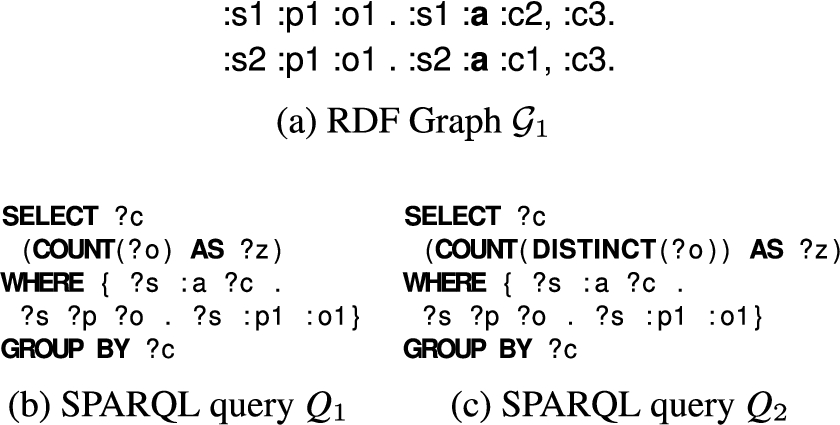
To illustrate, consider the query
3.2.Web preemption and SPARQL aggregate queries
Web preemption [14] is the capacity of a web server to suspend a running SPARQL query after a fixed quantum of time and resume the next waiting query. When suspending a query Q, a preemptable server saves the internal state of all operators of Q in a saved plan
However, Web preemption comes with overheads. The time taken by the suspend and resume operations represents the overhead in time of a preemptable server. The size of
For this purpose, a preemptable server only implements SPARQL operators that can be saved and resumed in constant time, i.e. preemptable operators. Based on the definition of tuple-at-a-time and full-relation operators [6], SPARQL operators can be classified into two groups: mapping-at-a-time and full-mappings operators.
Mapping-at-a-time operators such as SCAN, JOIN, UNION or BIND are implemented on the server. As they just need to manage one mapping at a time [6], these operators can be saved and resumed in constant time.11 Queries that can be evaluated using only mapping-at-a-time operators are supported by the preemptable server.
On the other hand, full-mappings operators require “seeing all or most of the mappings in memory at once” [6]. Consequently, they cannot be saved and resumed in constant time and are implemented on the client. For example, the ORDER BY is a full-mappings operator when the server has no choice but to materialize all the mappings before sorting them. This case typically arise when the ORDER BY operator is not combined with a LIMIT k operator, and the server has not the required sorted indexes. To evaluate a query that contains full-mappings operators, the client must decompose it into a set of subqueries supported by the server, evaluate each subquery separately, and recombine the intermediate results to produce the final query result. Such a decomposition can be extremely costly in terms of data transfer, number of calls to the server, and execution time.
Unfortunately, aggregate queries require a server-side operator that belongs to the full-mappings operators [6]. Consequently, there is no support on the server and aggregate queries must be decomposed.
![Evaluation of Q1 on G1 with regular web preemption [14].](https://content.iospress.com:443/media/sw/2022/13-4/sw-13-4-sw222842/sw-13-sw222842-g002.jpg)
Figure 2 illustrates how Web preemption processes the query
In a more general way, to evaluate
Reducing data transfer requires reducing
Problem Statement: Define a preemptable aggregation operator γ such that the complexity in time and space of suspending and resuming γ is bounded in constant time.22
4.Computing partial aggregations with web preemption
To build a preemptable evaluator for SPARQL aggregates, the presented approach relies on two key ideas: (i) First, Web preemption naturally creates a partition of mappings over time. Thanks to the decomposability of aggregate functions [26], partial aggregations can be computed server-side on each partition of mappings and recombined on the client. (ii) Second, to control the size of partial aggregations, the size of the quantum can be adjusted for aggregate queries.
In the following, the decomposability property of aggregate functions is presented, as well as how this property is used in the context of Web preemption.
4.1.Decomposable aggregate functions
Traditionally, the decomposability property of aggregate functions [26] ensures the correctness of the distributed computation of the aggregates [10]. This property is adapted for SPARQL aggregate queries in Definition 3.
Definition 3
Definition 3(Decomposable aggregation function).
An aggregate function f that used a list of expressions F is decomposable if for all non-empty multisets of solution mappings
In Definition 3, ⊎ denotes the multiset union as defined in [11]. Abusing the notation, we use a multiset of solution mappings Ω instead of the graph pattern P in Definition 2. Table 1 gives the decomposition of all SPARQL aggregate functions, where
Table 1
Decomposition of SPARQL aggregate functions with and without the DISTINCT modifier
| (a) Aggregate functions without the DISTINCT modifier | |||||
| SPARQL Aggregate functions | |||||
| COUNT | SUM | MIN | MAX | AVG | |
| COUNT | SUM | MIN | MAX | SaC | |
| h | |||||
| (b) Aggregate functions with the DISTINCT modifier | ||||
| SPARQL Aggregate functions | ||||
| CT | ||||
| h | COUNT | SUM | AVG | |
Fig. 3.
Evaluation of
To illustrate, consider the function
Decomposing SUM, COUNT, MIN and MAX is relatively simple, as partial aggregation results only need to be merged to produce the final query results. However, decomposing AVG and aggregate functions that use the DISTINCT modifier are more complex. Two auxiliary aggregate functions have been introduced, called SaC (SUM-and-COUNT) and CT (Collect), respectively. The SaC function collects the information required to compute an average, while the CT function collects a set of distinct values. They are defined as follows:
4.2.Partial aggregation with web preemption
Using a preemptive web server, the evaluation of a graph pattern P over
Definition 4
Definition 4(Partial aggregation).
Let F be a list of expressions, f an aggregate function and
Because a partial aggregation operates on
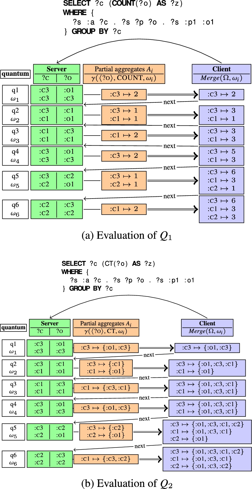
Figure 3(a) illustrates how a smart client computes
The duration of the quantum seriously impacts query processing using partial aggregations. Suppose that instead of six quanta of two mappings in Fig. 3(a), the server requires twelve quanta that produce one mapping each, therefore partial aggregations are useless. If the server requires two quanta that produce six mappings each, then only two partial aggregations
5.Count-distinct SPARQL aggregate queries
Count-distinct aggregate queries count the number of distinct elements in the multisets obtained after grouping. Query
As illustrated in Fig. 3(b), processing count-distinct aggregate queries requires transferring all elements from the server to the client before counting them. Moreover, these elements could be transferred several times if the query is processed over several quanta. For example,
To address this issue, we propose to estimate the number of distinct elements in a multiset rather than computing the exact count. Several probabilistic algorithms have been proposed [5,13,24] to estimate large cardinalities with a bounded memory. According to [9], the LinearCounting algorithm [24] achieves good accuracy, regardless of the cardinality. However, this algorithm is not attractive for large cardinalities, as it requires too much memory for an accurate estimate. Compared to the LinearCounting algorithm, the HyperLogLog (HLL) algorithm [13] is efficient for large cardinalities, both in terms of space complexity and accuracy. For instance, HLL can estimate cardinalities greater than
In the context of SPARQL aggregate queries, a good estimator must be accurate on both small and large cardinalities, and adapt its memory usage to cardinality. Indeed, aggregate queries deal with
5.1.HyperLogLog++
HLL++ is a probabilistic data structure that behaves like a set with two main operations:
1.
2.
The payload of a HLL++ set
To compute the cardinality of
To estimate the cardinality of
Fig. 4.
Approximate count-distinct for the
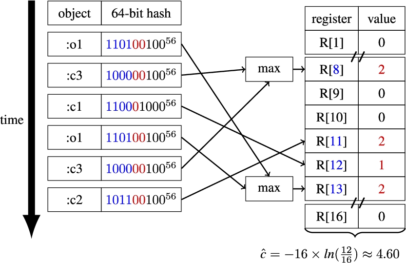
On its side, the LinearCounting algorithm relies on the fraction of empty registers (
To illustrate how HLL++ works, consider the example of Fig. 3(b) where the
5.2.Partial aggregations and HLL++
To estimate the number of distinct elements in a multiset, with a fixed error rate ϵ, we introduced a new aggregate function
Fig. 5.
Evaluation of the query
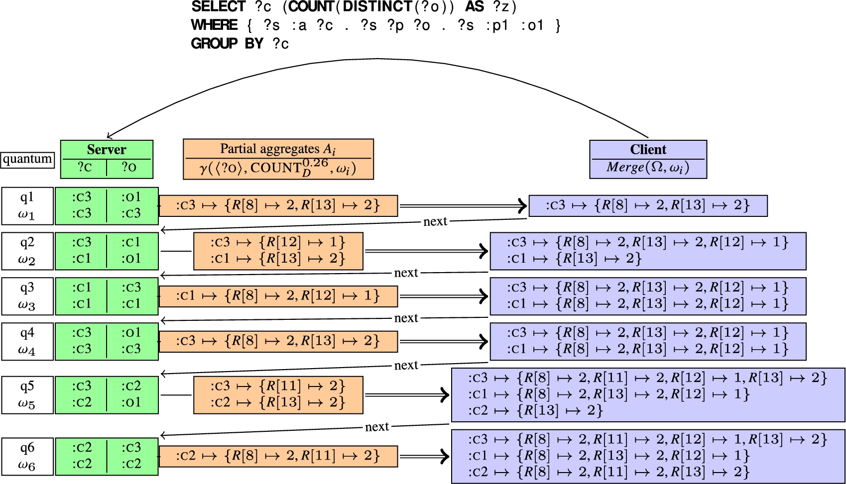
Figure 5(a) illustrates how a smart client computes
Compared to the HyperLogLog algorithm, HLL++ does not necessarily send all the registers to the client. To fit the memory efficiency criteria, HLL++ can store the array R using either a sparse or a full representation [9]. The sparse representation is used when most of the registers are empty and avoid transferring all registers to the client. Thus, for an error rate of 2%, the 1.5 KBytes per
To go back to our example, when the client receives the registers, it uses the
The duration of the quantum has a significant impact on the data transfer. Long quanta reduce data transfer as HLL++ sets are better used. However, long quanta are also likely to gather many
Algorithm 1:
Server-side evaluation of partial aggregates
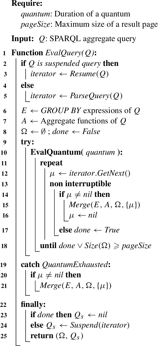
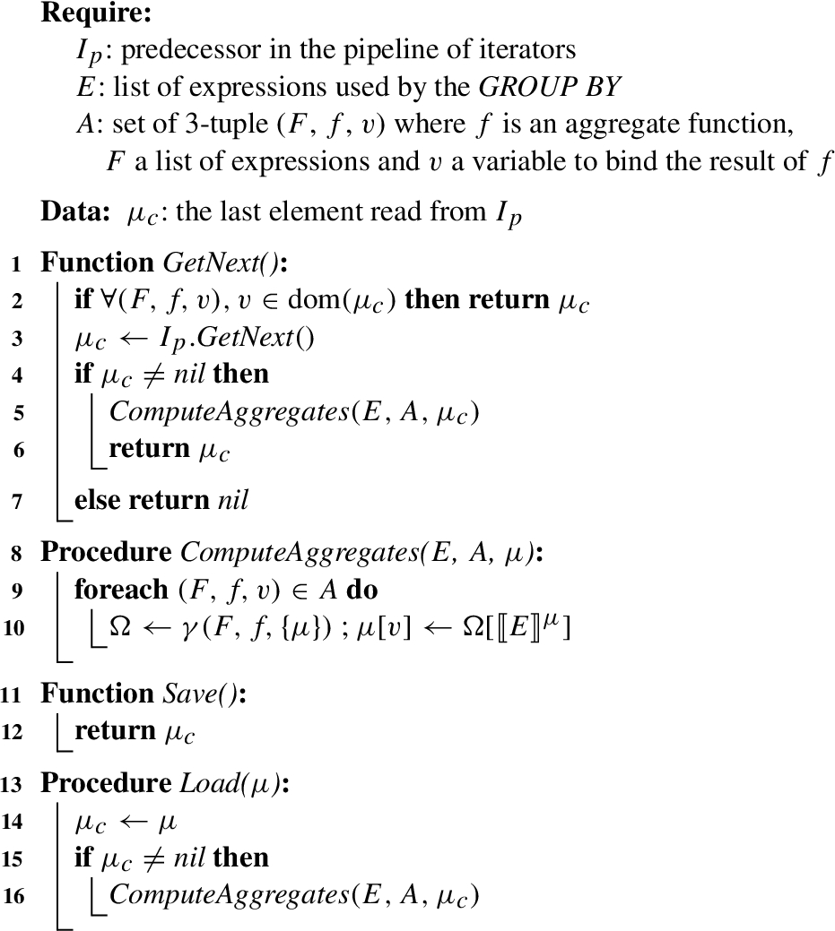
Algorithm 2:
Server-side preemptable SPARQL aggregates iterator
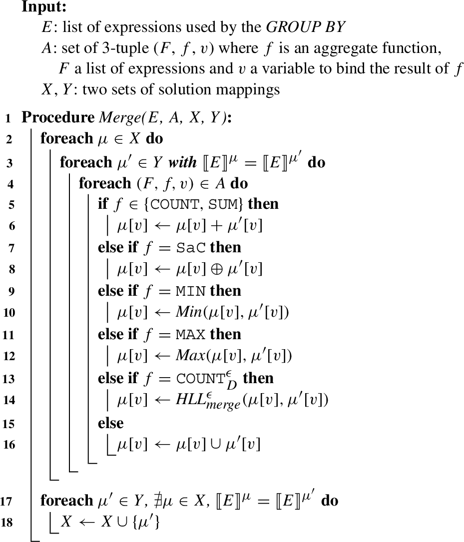
Algorithm 3:
Merge two sets of solution mappings, Y into X
6.Implementing decomposable aggregate functions
Algorithm 1 presents the general algorithm to compute partial aggregates on a preemptable server. To evaluate an aggregate query Q, the algorithm starts by building the physical plan of Q, i.e. a pipeline of preemptable iterators (Lines 3–6), that will be consumed by Algorithm 1. Algorithm 2 defines a new preemptable aggregates iterator for computing aggregate functions. When the GetNext() method is called, the new iterator consumes a solution mapping μ from its predecessor (Line 4), and computes aggregate functions on μ (Line 6). As aggregate functions are computed one mapping at a time, this iterator is preemptable, i.e. it can be saved and resumed in constant time. During a quantum, Algorithm 1 consumes solution mappings from the pipeline of iterators, and merges them into Ω (Lines 11–19), using the
The Merge(E,A,X,Y) operation merges two sets of solution mappings X and Y. For each
When the quantum is exhausted, the server waits for the non-interruptible section of Algorithm 1 to complete. Thus, no solution mappings are discarded, and the merge operation is guaranteed to be applied to every solution mapping. The non-interruptible section can block the program for at most the time to merge a single solution mapping in Ω, which can be done in constant time. Then, Algorithm 1 suspends the query Q, and sends the suspended query
To avoid the many-count distinct problem, i.e. exhaust the server memory, the size of Ω is bounded to a predefined constant
The evaluation of SPARQL aggregates on the server requires defining different parameters: the duration of a quantum, the maximum space allocated to the aggregation results, and the error rate ϵ when the
Algorithm 4:
Client-side evaluation of partial aggregates
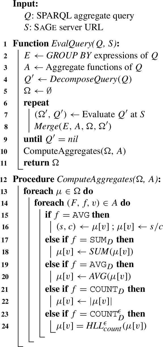
As the server computes only partial aggregates, it relies on the client to compute SPARQL aggregates, as shown in Algorithm 4. To execute a SPARQL aggregate query Q, the client first decomposes Q into
7.Experimental study
The purpose of the experimental study is to answer the following questions: (1) What is the data transfer reduction obtained with partial aggregations? (2) What is the speed up obtained with partial aggregations? (3) What is the impact of quantum on data transfer and execution time? (4) Does estimating the result of count-distinct queries reduce data transfer? (5) Does the observed error rate matches the theoretically guarantees provided by the HLL++ algorithm?
The partial aggregations approach has been implemented as an extension of the SaGe query engine.33 The SaGe server has been extended with the new operator described in Algorithm 2. Python SaGe-agg and SaGe-approx clients have been extended with Algorithm 4. SaGe-agg uses the
Dataset and queries The workload (SP) used in the experimental study is composed of 18 SPARQL aggregate queries extracted from the SPORTAL queries [8] (queries without ASK and FILTER). Most of the extracted queries use the DISTINCT modifier. SPORTAL queries are challenging because they aim to build VoID descriptions of RDF datasets.44 As reported in [8], most of the queries cannot complete over the DBpedia public server because of the quotas. Moreover, as depicted in Fig. 6, the SPORTAL queries return
To study the impact of the DISTINCT modifier on the aggregate queries execution, a new workload, denoted SP-ND, is defined by removing the DISTINCT modifier from the queries of SP.
Both the SP and the SP-ND workloads are run on synthetic and real-world datasets. For the synthetic datasets, the Berlin SPARQL Benchmark (BSBM) is used to generate three datasets of increasing size: BSBM-10, BSBM-100 and BSBM-1k. For the real-world dataset, a fragment of DBpedia v3.5.1 is used. The statistics of each dataset is detailed in Table 2.
Fig. 6.
Number of
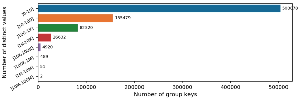
Table 2
Statistics of RDF datasets used in the experimental study
| RDF dataset | # Triples | # Subjects | # Predicates | # Objects | # Classes |
| BSBM-10 | 4 987 | 614 | 40 | 1 920 | 11 |
| BSBM-100 | 40 177 | 4 174 | 40 | 11 012 | 22 |
| BSBM-1k | 371 911 | 36 433 | 40 | 86 202 | 103 |
| DBpedia 3.5.1 | 100M | 2 835 701 | 35 168 | 26 840 695 | 342 |
Approaches The following approaches are compared:
– SaGe: corresponds to the SaGe query engine as defined in [14]. The SaGe server is configured with a maximum
– SaGe-agg: corresponds to the proposal defined in [7]. To be fairly compared with SaGe, SaGe-agg is configured as SaGe.
– SaGe-approx: corresponds to the extension of [7] defined in this paper. To be fairly compared with SaGe and SaGe-agg, SaGe-approx is configured as SaGe. To compute count-distinct queries, SaGe-approx uses an error rate
– TPF: corresponds to the TPF query engine [23]. The TPF server is configured with a page size of 10000 mappings and without Web caches. Data are stored using the HDT format. The TPF smart client is Comunica [21] (v1.9.4).
– Virtuoso: corresponds to the Virtuoso SPARQL endpoint [4] (v7.2.4). Virtuoso is configured without quotas and with a a single thread so that Virtuoso delivers complete results and can be fairly compared with other engines.
Servers configurations All experiments have been run on the Google Cloud Platform, on a n2-highmem-4 machine with 4 vCPU, 32 GBytes of RAM and a SSD local disk of 375 GBytes.
Evaluation metrics Presented results correspond to the average of three successive executions of the query workloads. (i) Data transfer: is the number of bytes transferred to the client when evaluating a query. (ii) Execution time: is the time between the start of the query and the production of the final results by the client. (iii) Error rate: is defined as the difference between the real cardinality c and the estimated cardinality
7.1.Experimental results
7.1.1.Data transfer and execution time over BSBM datasets
Figure 7 presents the data transfer and the execution time over BSBM-10, BSBM-100 and BSBM-1k. In this experiment, the SaGe server is configured with a time quantum of 150 ms. The plots on the left detail the results for the SP workload, while the plots on the right detail the results for the SP-ND workload.
Fig. 7.
Data transfer and execution time for BSBM-10, BSBM-100 and BSBM-1k, when running the SP (left) and SP-ND (right) workloads.
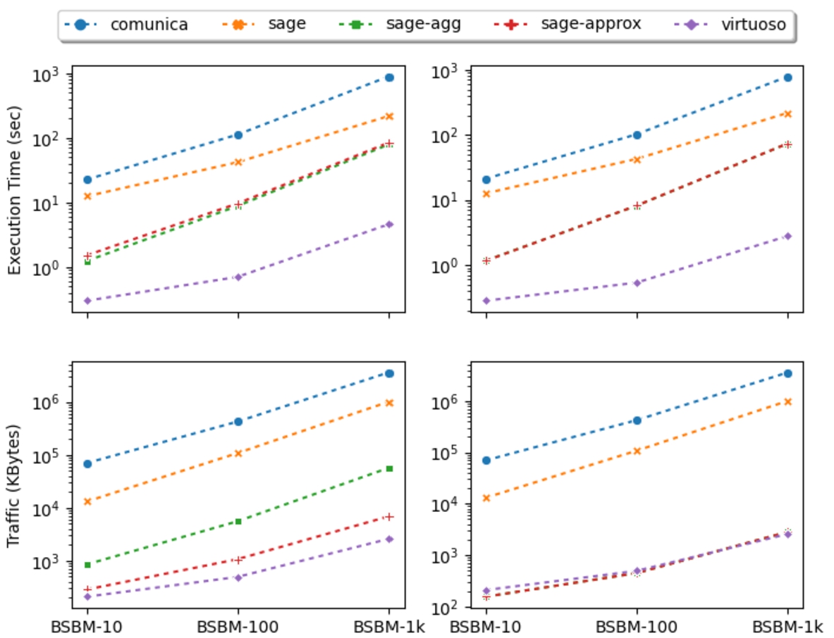
As expected, Virtuoso without quota performs the best in terms of data transfer and execution time. On the other hand, TPF offers the worst performance as it does not support projections nor joins on the server-side. As a result, TPF transfers a large number of intermediate results and sends many HTTP requests to the server, which has a significant impact on query execution time. Although both SaGe and TPF evaluate SPARQL aggregate queries on the client-side, SaGe delivers better performance than TPF because it supports projections and joins on the server.
Compared to SaGe, SaGe-agg and SaGe-approx drastically reduce data transfer but do not improve the execution time, because partial aggregations do not increase the scanning speed on the disk. When comparing the performance of SaGe-agg and SaGe-approx on the two workloads, we can observe that query processing without the distinct modifier (on the right) is much more efficient in terms of data transfer than with the distinct modifier (on the left).
Without the distinct modifier, SaGe-agg and SaGe-approx are equivalent and transfer only one number per
For queries that use the distinct modifier, SaGe-agg has to transfer all terms observed during a quantum. The only optimization that can be done to reduce data transfer is to remove the duplicates observed during the same quantum. However, those observed during different quanta cannot be removed. Compared to SaGe-agg, SaGe-approx significantly improves the evaluation of count-distinct queries in terms of data transfer. For each
7.1.2.Data transfer and execution time over DBPedia
To confirm the results observed on the synthetic datasets, we ran the SP workload on a fragment of DBpedia, using both SaGe-agg, SaGe-approx and Virtuoso. The quantum for SaGe-agg and SaGe-approx has been set to 30 seconds. The results are shown in Fig. 8, where the queries (Q2, Q3, Q4, Q5, Q7, Q8, Q9, Q10, Q12, Q13, Q15, Q16) labeled in blue are the ones that use the distinct modifier.
Fig. 8.
Performance obtained in terms of execution time and data transfer with the SP workload on the DBpedia dataset.
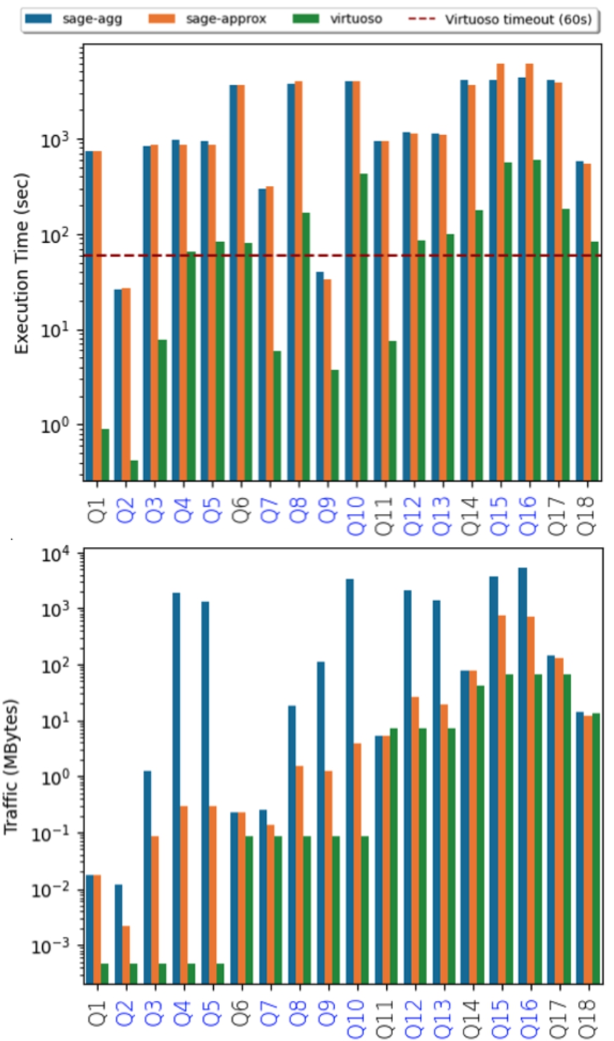
As expected, Virtuoso delivers the best performance in terms of data transfer and execution time. In terms of execution time, the differences between Virtuoso and both SaGe-agg and SaGe-approx are mainly due to a lack of query optimizations in the SaGe-agg and SaGe-approx implementations; no projection push-down, no merge-joins, etc. In terms of data transfer, Virtuoso is optimal as it computes the full aggregations on the server-side and transfers only the final results. Compared to Virtuoso, SaGe-agg and SaGe-approx perform only partial aggregations on the server-side. Nevertheless, Virtuoso cannot ensure that all queries terminate under quotas. The red dotted line in Fig. 8 corresponds to a quota of 60 s. As we can see, queries Q5, Q6, Q8, Q10, Q12, Q13, Q14, Q15, Q16, Q17 and Q18 do not terminate, i.e. two thirds of the queries are interrupted after 60 s and return no results.
Compared to Virtuoso, the SaGe server does not interrupt queries. The queries are just suspended after a time quantum and resumed later. Consequently, both SaGe-agg and SaGe-approx ensure termination of all queries. Finally, as expected, SaGe-approx drastically improves performance in terms of data transfer on large RDF datasets.
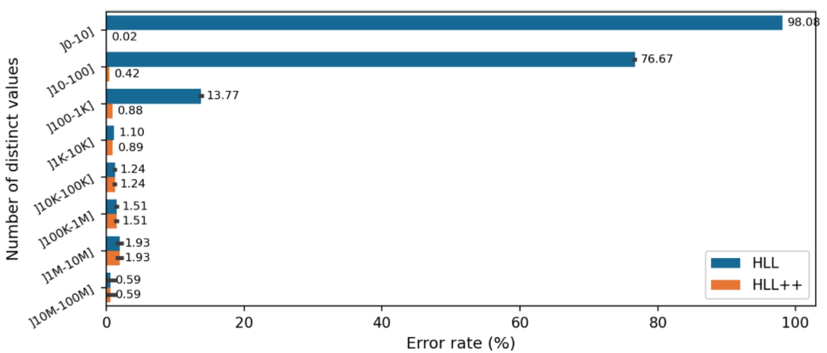
7.1.3.Error rates over DBpedia
SaGe-approx approximates the result of count-distinct queries and hence, there is a potential for error. To ensure that the theoretical guarantees on the error rate holds in practice, we measured the error rate for each
Fig. 9.
Average error rate for the
7.1.4.Impact of time quantum
To study the impact of the quantum on data transfer and query execution time, the two workloads have been run with different time quantum. Figure 10 reports the results of running SaGe, SaGe-agg, SaGe-approx and Virtuoso with a quantum of 75 ms, 150 ms, 1.5 sec and 15 sec on BSBM-1k. The plots on the left detail the results for the SP workload and on the right the SP-ND workload.
Fig. 10.
Quantum impact on the execution of SP (left) and SP-ND (right) workloads on the BSBM-1k dataset.
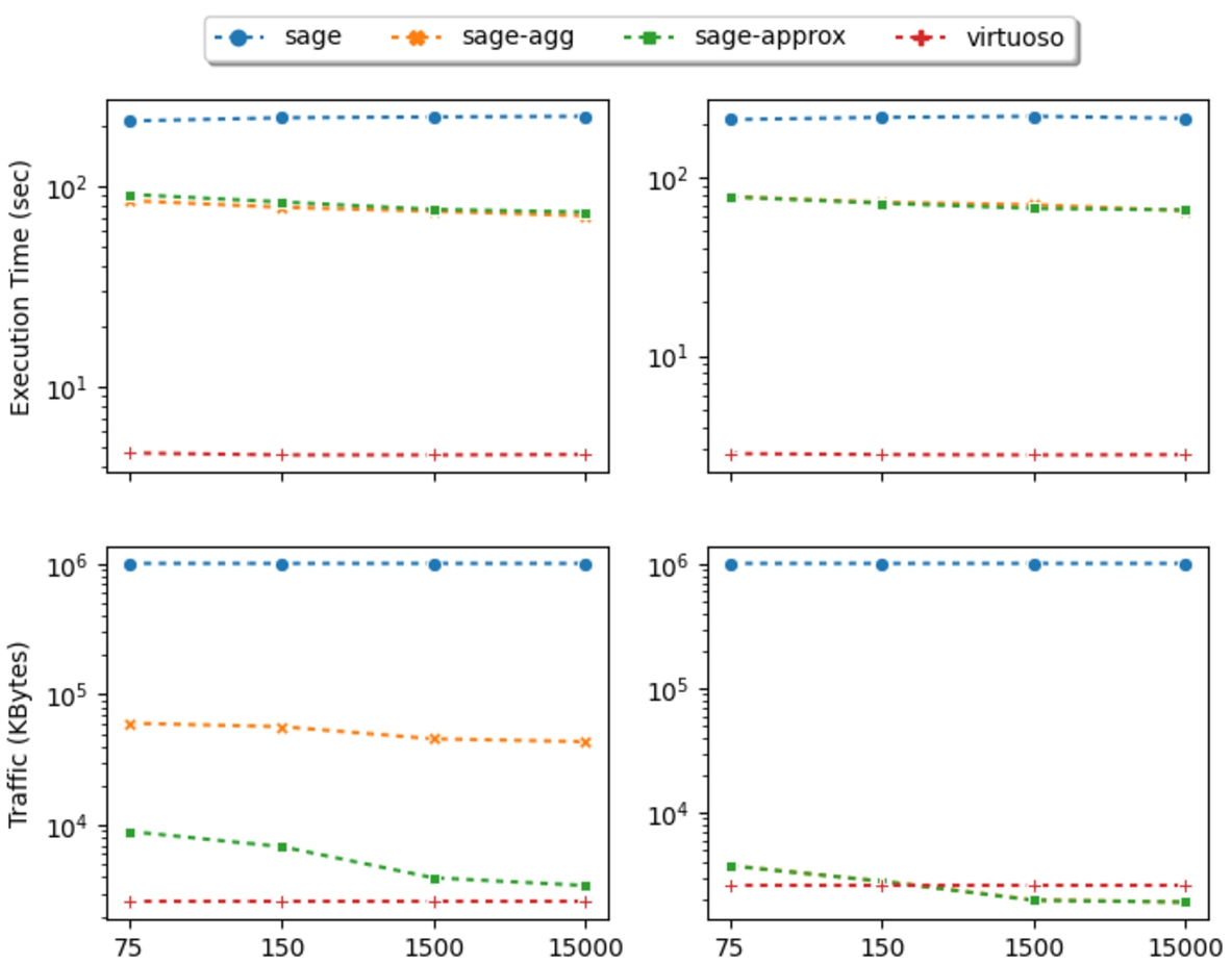
As we can see, increasing the quantum does not significantly improve the execution time. The speed of scans does not change whatever the value of the quantum. However, increasing the quantum reduces the data transfer for SaGe-agg and SaGe-approx on both workloads. Indeed, increasing the quantum allows a better use of partial aggregations. The less often a query is interrupted, the less likely it is to transfer the same
Finally, we can observe that SaGe-agg is less impacted by the quantum duration than SaGe-approx. Even if higher quanta allow to deduplicate more terms, the number of elements transferred by SaGe-agg remains important and dominates the data transfer.
8.Discussion
The results show that using probabilistic data structures to compute count-distinct queries significantly reduces data transfer. However, the current implementation still has poor performance in terms of execution time, which limits its application to very large knowledge graphs such as Wikidata or DBpedia. As mentioned in the experimental study, these performance issues are due to a lack of query optimizations on the SaGe server. The simple application of state-of-art optimization techniques, including filter and projection push-down, aggregate push-down or merge-joins should significantly improve performance.
Moreover, the current approach only proposes to improve the evaluation of count-distinct queries. To evaluate avg-distinct and sum-distinct queries, the server still has to transfer all the elements to the client. Unfortunately, to the best of our knowledge, there is currently no probabilistic data structure that supports estimating a distinct sum.
Finally, to avoid the many-count distinct problem, we currently rely on Web preemption. By limiting the memory dedicated to the aggregation results, we ensure that a quantum only processes a limited number of
9.Conclusion and future works
In this paper, we have extended the partial aggregation operator presented in [7] in order to improve the evaluation of count-distinct aggregate queries. We have shown how the decomposability property of the HyperLogLog++ algorithm can be used to integrate HyperLogLog++ sketches in our framework. We have demonstrated experimentally that using HyperLogLog++ sketches drastically reduce data transfer for SPARQL count-distinct queries. Compared to related approaches, the presented solution ensures that all
The next step is to extend this approach to handle large knowledge graphs. One way to scale up is to parallelize the evaluation of SPARQL aggregate queries. Currently, Web preemption does not support intra-query parallelization techniques. Defining how to suspend and resume parallel scans is clearly part of our research agenda. Finally, addressing the many-count distinct problem on the server-side could reduce the data transfer, and the memory consumption on both the server and the client.
Notes
1 A SCAN can be resumed in
2 In this paper, for simplicity, only aggregate queries with Basic Graph Patterns and no OPTIONAL clauses are considered.
Acknowledgements
This work is supported by the ANR DeKaloG (Decentralized Knowledge Graphs) project, ANR-19-CE23-0014 – AAPG2019 – program CE23.
References
[1] | S. Auer, J. Demter, M. Martin and J. Lehmann, LODStats – An extensible framework for high-performance dataset analytics, in: International Conference on Knowledge Engineering and Knowledge Management, Springer, (2012) , pp. 353–362. doi:10.1007/978-3-642-33876-2_31. |
[2] | A. Azzam, J.D. Fernández, M. Acosta, M. Beno and A. Polleres, SMART-KG: Hybrid shipping for SPARQL querying on the web, in: Proceedings of the Web Conference 2020, (2020) , pp. 984–994. doi:10.1145/3366423.3380177. |
[3] | C. Buil-Aranda, A. Polleres and J. Umbrich, Strategies for executing federated queries in SPARQL 1.1, in: International Semantic Web Conference, Springer, (2014) , pp. 390–405. doi:10.1007/978-3-319-11915-1_25. |
[4] | O. Erling and I. Mikhailov, RDF support in the Virtuoso DBMS, in: Networked Knowledge-Networked Media, Springer, (2009) , pp. 7–24. doi:10.1007/978-3-642-02184-8_2. |
[5] | C. Estan, G. Varghese and M. Fisk, Bitmap algorithms for counting active flows on high speed links, in: Proceedings of the 3rd ACM SIGCOMM Conference on Internet Measurement, (2003) , pp. 153–166. doi:10.1145/948205.948225. |
[6] | H. Garcia-Molina, J.D. Ullman and J. Widom, Database Systems: The Complete Book, 2nd edn, Prentice Hall Press, USA, (2008) . doi:10.5555/1450931. |
[7] | A. Grall, T. Minier, H. Skaf-Molli and P. Molli, Processing SPARQL aggregate queries with web preemption, in: European Semantic Web Conference, Springer, (2020) , pp. 235–251. doi:10.1007/978-3-030-49461-2_14. |
[8] | A. Hasnain, Q. Mehmood, S.S. e Zainab and A. Hogan, SPORTAL: Profiling the content of public SPARQL endpoints, International Journal on Semantic Web and Information Systems (IJSWIS) 12: (3) ((2016) ), 134–163. doi:10.4018/IJSWIS.2016070105. |
[9] | S. Heule, M. Nunkesser and A. Hall, Hyperloglog in practice: Algorithmic engineering of a state of the art cardinality estimation algorithm, in: Proceedings of the 16th International Conference on Extending Database Technology, (2013) , pp. 683–692. doi:10.1145/2452376.2452456. |
[10] | P. Jesus, C. Baquero and P.S. Almeida, A survey of distributed data aggregation algorithms, IEEE Communications Surveys & Tutorials 17: (1) ((2014) ), 381–404. doi:10.1109/COMST.2014.2354398. |
[11] | M. Kaminski, E.V. Kostylev and B.C. Grau, Query nesting, assignment, and aggregation in SPARQL 1.1, ACM Transactions on Database Systems (TODS) 42: (3) ((2017) ), 1–46. doi:10.1145/3083898. |
[12] | K. Li and G. Li, Approximate query processing: What is new and where to go?, Data Science and Engineering 3: (4) ((2018) ), 379–397. doi:10.1007/s41019-018-0074-4. |
[13] | F. Meunier, O. Gandouet, É. Fusy and P. Flajolet, Hyperloglog: The analysis of a near-optimal cardinality estimation algorithm, Discrete Mathematics & Theoretical Computer Science ((2007) ). doi:10.46298/dmtcs.3545. |
[14] | T. Minier, H. Skaf-Molli and P. Molli, SaGe: Web preemption for public SPARQL query services, in: The World Wide Web Conference, (2019) , pp. 1268–1278. doi:10.1145/3308558.3313652. |
[15] | J. Pérez, M. Arenas and C. Gutierrez, Semantics and complexity of SPARQL, ACM Transactions on Database Systems (TODS) 34: (3) ((2009) ), 1–45. doi:10.1145/1567274.1567278. |
[16] | A. Schätzle, M. Przyjaciel-Zablocki, S. Skilevic and G. Lausen, S2rdf: Rdf querying with sparql on spark, Proc. VLDB Endow. 9: (10) ((2016) ). doi:10.14778/2977797.2977806. |
[17] | M. Schmidt, M. Meier and G. Lausen, Foundations of SPARQL query optimization, in: Proceedings of the 13th International Conference on Database Theory, (2010) , pp. 4–33. doi:10.1145/1804669.1804675. |
[18] | A. Singh, S. Garg, R. Kaur, S. Batra, N. Kumar and A.Y. Zomaya, Probabilistic data structures for big data analytics: A comprehensive review, Knowledge-Based Systems 188: ((2020) ), 104987. doi:10.1016/j.knosys.2019.104987. |
[19] | A. Soulet and F.M. Suchanek, Anytime large-scale analytics of linked open data, in: International Semantic Web Conference, Springer, (2019) , pp. 576–592. doi:10.1007/978-3-030-30793-6_33. |
[20] | H. Steve and S. Andy, SPARQL 1.1 query language, in: Recommendation W3C, (2013) . |
[21] | R. Taelman, J. Van Herwegen, M. Vander Sande and R. Verborgh, Comunica: A modular SPARQL query engine for the web, in: International Semantic Web Conference, Springer, (2018) , pp. 239–255. doi:10.1007/978-3-030-00668-6_15. |
[22] | D. Ting, Approximate distinct counts for billions of datasets, in: Proceedings of the 2019 International Conference on Management of Data, (2019) , pp. 69–86. doi:10.1145/3299869.3319897. |
[23] | R. Verborgh, M. Vander Sande, O. Hartig, J. Van Herwegen, L. De Vocht, B. De Meester, G. Haesendonck and P. Colpaert, Triple pattern fragments: A low-cost knowledge graph interface for the web, Journal of Web Semantics 37: ((2016) ), 184–206. doi:10.1016/j.websem.2016.03.003. |
[24] | K.Y. Whang, B.T. Vander-Zanden and H.M. Taylor, A linear-time probabilistic counting algorithm for database applications, ACM Transactions on Database Systems (TODS) 15: (2) ((1990) ), 208–229. doi:10.1145/78922.78925. |
[25] | Q. Xiao, S. Chen, M. Chen and Y. Ling, Hyper-compact virtual estimators for big network data based on register sharing, in: Proceedings of the 2015 ACM SIGMETRICS International Conference on Measurement and Modeling of Computer Systems, (2015) , pp. 417–428. doi:10.1145/2745844.2745870. |
[26] | W.P. Yan and P.B. Larson, Eager aggregation and lazy aggregation, Group 1: ((1995) ), G2. |

