
Filling the gaps: A multiple imputation approach to estimating aging curves in baseball
Abstract
In sports, an aging curve depicts the relationship between average performance and age in athletes’ careers. This paper investigates the aging curves for offensive players in Major League Baseball. We study this problem in a missing data context and account for different types of dropouts of baseball players during their careers. We employ a multiple imputation framework for multilevel data to impute the player performance associated with the missing seasons, and estimate the aging curves based on the imputed datasets. We then evaluate the effects of different dropout mechanisms on the aging curves through simulation, before applying our method to analyze MLB player data from past seasons. Results suggest an overestimation of the aging curves constructed without considering the unobserved seasons, whereas estimates obtained from multiple imputation address this shortcoming.
1Introduction
The rise and fall of an athlete is a popular topic of discussion in the sports media today. Questions regarding whether a player has reached their peak, is past their prime, or is good enough to remain in their respective professional league are often seen in different media outlets such as news articles, television debate shows, and podcasts. The average performance of players by age throughout their careers is visually represented by an aging curve. This graph typically consists of a horizontal axis representing a time variable (usually age or season) and a vertical axis showing a performance metric at each time point in a player’s career.
One significant challenge associated with the study of aging curves in sports is survival bias, as pointed out by Lichtman (2009), Turtoro (2019), Judge (2020a), and Schuckers et al. (2023). In particular, the aging effects are not often determined from a full population of athletes (i.e., all players who have ever played) in a given league. That is, only players that are good enough to remain are observed; whereas those who might be involved, but do not actually participate or are not talented enough to compete, are being completely disregarded. This very likely results in an overestimation of the aging curves.
As such, player survivorship and dropout can be viewed as a missing data problem. There are several distinct cases of player absence from professional sport at different points in their careers. Early on, teams may elect to assign their young prospects to their minor/development league affiliates for several years of nurture. Many of those players would end up receiving a call-up to join the senior squad, when the team believes they are ready. During the middle of a player’s career, a nonappearance could occur due to various reasons. Injury is unavoidable in sports, and this could cost a player at least one year of their playing time. Personal reasons such as contract situation and more recently, concerns regarding a global pandemic, could also lead to athletes sitting out a season. Later on, a player, by either their choice or their team’s choice, might head for retirement because they cannot perform at a level like they used to, leading to unobserved seasons that could have been played.
The primary aim of this paper is to apply missing data techniques to the estimation of aging curves. In doing so, we focus on baseball and pose the following research question: What would the aging curve look like if all players competed in every season within a fixed range of age? In other words, what would have happened if a player who was forced to retire from their league at a certain age had played a full career? The manuscript continues with a review of existing literature on aging curves in baseball and other sports in Section 2. Next, we describe our data and methods used to perform our analyses in Section 3. After that, our approach is implemented through simulation and analyses of real baseball data in Sections 4 and 5. Finally, in Section 6, we conclude with a discussion of the results, limitations, and directions for future work.
2Literature review
To date, we find a considerable amount of previous work related to aging curves and career trajectory of athletes. This body of work consists of several key themes, a wide array of statistical methods, and applications in many sports besides baseball such as basketball, hockey, and track and field, to name a few.
A typical notion in the baseball aging curves literature is the assumption of a quadratic form for modeling the relationship between performance and age. Morris (1983) looked at Ty Cobb’s batting average trajectory using parametric empirical Bayes and used shrinkage methods to obtain a parabolic curve for Cobb’s career performance. Albert (1992) proposed a quadratic random effects log-linear model for smoothing a batter’s home run rates throughout their career. Berry et al. (1999) implemented a nonparametric method to estimate the age effect on performance in baseball, hockey, and golf. However, Albert (1999) weighed in on this nonparametric approach and questioned the assumptions that the peak age and periods of growth and decline are the same for all players. Albert (1999) ultimately preferred a second-degree polynomial function for estimating age effect in baseball, which is a parametric model. Continuing his series of work on aging trajectories, Albert (2002) proposed a Bayesian exchangeable model for baseball hitting performance. This approach combined quadratic regression estimates and assumes similar careers for players born in the same decade. Fair (2008) and Bradbury (2009) both used a fixed-effects regression to examine age effects in the MLB, also assuming a quadratic aging curve form. A major drawback of Bradbury (2009)’s study is that the analysis only considered players with longer baseball careers.
In addition to baseball, studies on aging curves have also been conducted for other sports. Early on, Moore (1975) looked at the association between age and running speed in track and field and produced aging curves for different running distances using an exponential model. Fair (1994) and Fair (2007) studied the age effects in track and field, swimming, chess, and running, in addition to their latter work in baseball, as mentioned earlier. In triathlon, Villaroel et al. (2011) assumed a quadratic relationship between performance and age, as many have previously considered. As for basketball, Page et al. (2013) used a Gaussian process regression in a hierarchical Bayesian framework to model age effect in the NBA. Additionally, Lailvaux et al. (2014) used NBA and WNBA data to investigate and test for potential sex differences in the aging of comparable performance indicators. Vaci et al. (2019) applied Bayesian cognitive latent variable modeling to explore aging and career performance in the NBA, accounting for player position and activity level. In tennis, Kovalchik (2014) studied age and performance trends in men’s tennis using change point analysis.
Another convention in the aging curve modeling literature is the assumption of discrete observations. Specifically, most researchers use regression modeling and consider a data measurement for each season played throughout a player’s career. In contrast to previous approaches, Wakim & Jin (2014) took a different route and considered functional data analysis as the primary tool for modeling MLB and NBA aging curves. This is a continuous framework which treats the entire career performance of an athlete as a smooth function. In a similar functional data setting, Leroy et al. (2018) investigated the performance progression curves in swimming.
A subset of the literature on aging and performance in sports specifically studies the question: At what age do athletes peak? Schulz & Curnow (1988) looked at the age of peak performance for track and field, swimming, baseball, tennis, and golf. A follow-up study to this work was done by Schulz et al. (1994), where the authors focused on baseball and found that the average peak age for baseball players is between 27 and 30, considering several performance measures. Later findings on baseball peak age also showed consistency with the results in Schulz et al. (1994). Fair (2008) determined the peak-performance age in baseball to be 28, whereas Bradbury (2009) determined that baseball hitters and pitchers reach the top of their careers at about 29 years old. In soccer, Dendir (2016) determined that the peak age for footballers in the top leagues falls within the range of 25 to 27.
The idea of player survivorship is only mentioned in a small number of articles. To our knowledge, not many researchers have incorporated missing data methods into the estimation of aging curves to account for missing but observable athletes. Schulz et al. (1994) and Schell (2005) noted the selection bias problem with estimating performance averages by age in baseball, as better players tend to have longer career longevity. Schall & Smith (2000) predicted survival probabilities of baseball players using a logit model, and examined the link between first-year performance and career length. Lichtman (2009) studied different aging curves for different eras and groups of players after correcting for survival bias, and showed that survival bias results in an overestimation of the age effects. In other words, the average performance-level at any given age is overestimated when survival bias is not considered. Judge (2020a) also examined survival bias and found that the slope between age and performance is underestimated when using only surviving players in the estimation. We note that Judge (2020a) studied how the slope of the aging curve is affected by survival bias, whereas Lichtman (2009) investigated the bias in the average performance level at each specific age (i.e. the height of the curve) which is similar to our goal in this paper. In analyzing NHL player aging, Brander et al. (2014) applied their quadratic and cubic fixed-effects regression models to predict performance for unobserved players in the data.
Recently, researchers have noticed the benefits of accounting for missing data in modeling performance in sports. Stival et al. (2023) used a latent class matrix-variate state-space framework to analyze runners’ careers, and found that missing data patterns greatly contribute to the prediction of performance. Perhaps the most closely related approach to our work is that by Schuckers et al. (2023), which considered different regression and imputation frameworks for estimating the aging curves in the National Hockey League (NHL). First, they investigated different regression approaches including spline, quadratic, quantile, and a delta plus method, which is an extension to the delta method previously studied by Lichtman (2009), Turtoro (2019), and Judge (2020b). This paper also proposed an imputation approach for aging curve estimation, and ultimately concluded that the estimation becomes stronger when accounting for unobserved data, which addresses a major shortcoming in the estimation of aging curves. Säfvenberg (2022) modified Schuckers et al. (2023)’s imputation algorithm to study aging trajectory in Swedish football.
However, it appears that the aging curves in the aforementioned papers are constructed without taking into account the variability as a result of imputing missing data. This could be improved by applying multiple imputation rather than considering only one imputed dataset. As pointed out by Gelman & Hill (2006) (Chapter 25), conducting only a single imputation essentially assumes that the filled-in values correctly estimate the true values of the missing observations. Yet, there is uncertainty associated with the missingness, and multiple imputation can incorporate the missing data uncertainty and provide estimates for the different sources of variability.
3Methods
3.1Data collection
In the forthcoming analyses, we rely on one primary source of publicly available baseball data: the Lahman baseball database (Lahman 2021). Created and maintained by Sean Lahman, this database contains pitching, hitting, and fielding information for Major League Baseball players and teams dating back to 1871. The data are available in many different formats, and the Lahman package in R (Friendly et al. 2022, R Core Team 2023) is used for our investigation.
Due to our specific purpose of examining the aging curves for baseball offensive players, we consider the following datasets from the Lahman library: Batting, which provides season-by-season batting statistics for baseball players; and People, which contains the date of birth of each player, allowing us to calculate their age for each season played. In each table, an athlete is identified with their own playerID, hence we use this attribute as a joining key to merge the two tables together. A player’s age for a season is determined as their age on June 30, and we apply the formula suggested by Marchi et al. (2018) for age adjustment based on one’s birth month.
Throughout this paper, we consider on-base plus slugging (OPS), which combines a hitter’s ability to reach base and power-hitting, as the baseball offensive performance measure. We normalize the OPS for all players and then apply an arcsine transformation to ensure a reasonable range for the OPS values when conducting simulation and imputation. We also assume a fixed length for a player’s career, ranging from age 21 to 39. In terms of sample restriction, we observe all player-seasons with at least 100 plate appearances, which means a season is determined as missing if one’s plate appearances is below that threshold.
3.2Multiple imputation
Multiple imputation (Rubin 1987) is a popular statistical procedure for addressing the presence of incomplete data. The goal of this approach is to replace the missing data with plausible values to create multiple completed datasets. These completed datasets can each then be analyzed and results are combined across the imputed versions. Multiple imputation consists of three steps. First, based on an appropriate imputation model, m completed copies of the dataset are created by filling in the missing values. Next, m analyses are performed on each of the m completed datasets. Finally, the results from each of the m datasets are pooled together using Rubin’s rules (Little & Rubin 1987).
It is important to understand the reasons behind the missingness when applying multiple imputation to handle incomplete data. Generally, there are three types of missing data: missing completely at random (MCAR), missing at random (MAR), and missing not at random (MNAR) (Rubin 1976). MCAR occurs when a missing observation is statistically independent of both the observed and unobserved data. In the case of MAR, the missingness is associated only with the observed and not with the unobserved data. When data are MNAR, the probability of missingness is related to both observed and unobserved data.
Among the tools for performing multiple imputation, multivariate imputations by chained equation (MICE) ( & Groothuis-Oudshoorn 1999) is a flexible, robust, and widely used method. This algorithm imputes missing data via an iterative series of conditional models. In each iteration, each incomplete variable is filled in by a separate model of all the remaining variables. The iterations continue until apparent convergence is reached.
Here we implement the MICE framework in R via the popular mice package (van Buuren & Groothuis-Oudshoorn 2011). Moreover, we focus on multilevel multiple imputation, due to the hierarchical structure of our data. Specifically, we consider multiple imputation by a two-level normal linear mixed model with heterogeneous within-group variance (Kasim & Raudenbush 1998). In context, our data consist of baseball seasons (ages) which are nested within the class variable, player; and the season-by-season performance is considered to be correlated for each athlete. The described imputation model can be specified as the 2l.norm method available in the mice library.
4Simulation
In this simulation, we demonstrate our aging curve estimation approach with multiple imputation, and evaluate how different types of player dropouts affect the curve. There are three steps to our simulation. First, we fit a model for the performance-age relationship and use its output to generate reasonable careers for baseball players. For computational simplicity, we consider a mixed-effects model that assumes the same aging curve for all players and allowing for a random shift across players. Next, we generate missing data by dropping players from the full dataset based on different criteria, and examine how the missingness affects the original aging curve obtained from fully observed data. Finally, we apply multiple imputation to obtain completed datasets and assess how close the imputed aging curves are to the true curve based on fully observed data.
4.1Generating player careers
We fit a mixed-effects model using the player data described in Section 3.1. Our goal is to obtain the variance components of the fitted model to simulate baseball player careers. The model of interest is of the following form:
4.2Generating missing data
After obtaining reasonable simulated careers for baseball players, we create different types of dropouts and examine how they lead to deviations from the fully observed aging curve. We consider the following cases of player dropout from the league:
1 Dropout players with 4-year OPS average below a certain threshold, say 0.55.
2 Dropout players with OPS average from age 21 (start of career) to 25 of less than 0.55.
3 25% of the players randomly retire at age 30.
4 Players with OPS average below 0.55 between age 21 and 25 are not being promoted until age 25.
For the first two scenarios, the missingness mechanism is MAR, since players get removed due to low previously observed performance. Specifically, for case (2), all player-seasons at the beginning at their career between age 21 and 25 are observed, and low-performing players during this playing period are dropped. Dropout case (3) falls under MCAR, since athletes are selected completely at random to retire without considering past or future offensive production. Case (4) illustrates MNAR, since our consideration is that players who have low OPS at the beginning do not make it into the major league until they turn 25. Here, the dropped OPS values are what their OPS would have been if they played, but because it would have been so low, they do not get promoted until the age cutoff of 25.
Figure 1 displays the average OPS aging curve for all baseball players obtained from the original data with no missingness, along with the aging curves constructed based on data with only the surviving players associated with the aforementioned dropout mechanisms. For each dropout case, the corresponding curve is based on the average OPS at each age aggregated across all players that remain after dropout. These are smoothed curves obtained from loess model fits, and we use mean absolute error (MAE) to evaluate the discrepancy between the dropout and true aging curves.
Fig. 1
Comparison of the average aging curves constructed with the full simulated data and different cases of dropouts (without imputation). The dropout mechanisms presented are (1) dropping players with any 4-year OPS average below 0.55; (2) dropping players with OPS average between age 21 and 25 of less than 0.55; (3) randomly removing 25% of the players at age 30; and (4) players with low OPS average between age 21 and 25 are not being promoted until age 25. Results shown here are for 1,000 player-careers generated from simulation.
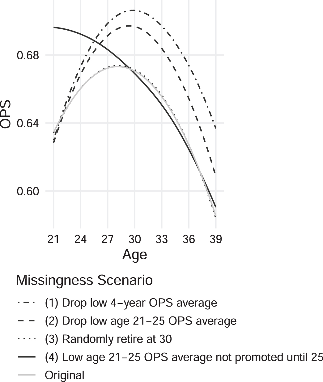
It is clear that randomly removing players have minimal effect on the aging curve, as the curve obtained from (3) and the original curve essentially overlap (MAE = 7.42 × 10⁻⁴). On the other hand, a positive shift from the fully observed curve occurs for the remaining two cases of dropout based on OPS average (MAE = 0.031 for (1) and MAE = 0.019 for (2)). This means the aging curves with only the surviving players are overestimated in the presence of missing data due to past performance. More specifically, the estimated player performance drops off faster as they age when considering missing data than when it is estimated with only complete case analysis (i.e. only considering observed seasons). As for case (4), when low-performing players are not being promoted until age 25 and only good players are observed before age 25, we observe an overestimation at the beginning of player’s career. Aside from overestimating the aging curve, ignoring player dropout also pushes the estimated performance peak to a later point (29 years old) in a player’s career.
4.3Imputation
Next, we implement the multiple imputation with a hierarchical structure procedure described in Section 3 to the cases of dropout that shifts the aging effect on performance. We perform m = 5 imputations with each made up of 30 iterations of the MICE algorithm, and apply Rubin’s rules for combining the imputation estimates. The following results are illustrated for dropout mechanism (2), where players with a low OPS average at the start of their careers (ages 21–25) are forced out of the league.
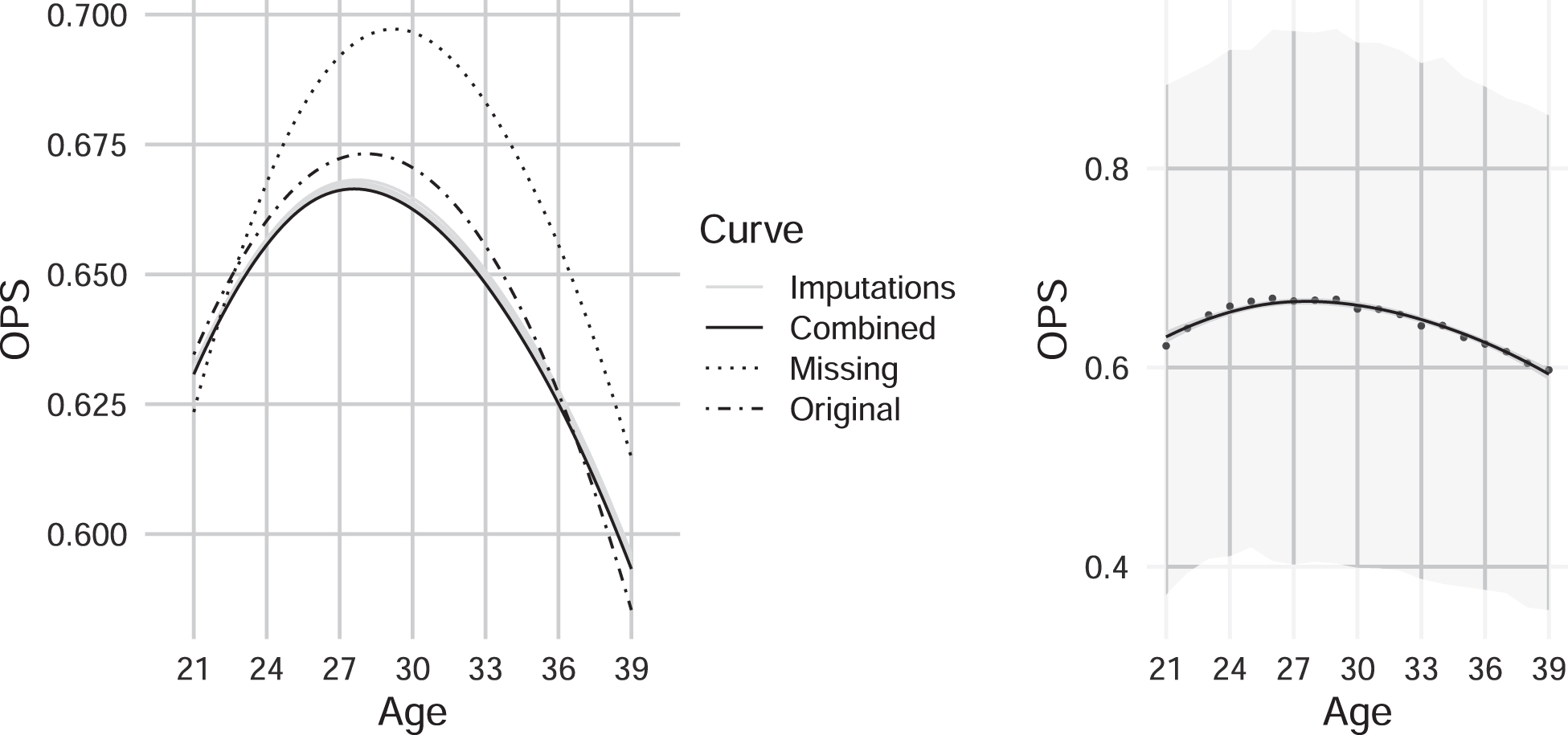
Figure 2 (left) shows smoothed fitting loess aging curves for all 5 imputations and a combined version of them, in addition to the curves constructed with fully observed and only surviving players data. Similar to Fig. 1, these curves are obtained by averaging the OPS for each age across all players with non-missing OPS values. The 95% confidence interval for the mean OPS at each age point in the combined curve obtained from Rubin’s rules is further illustrated in Fig. 2 (right). It appears that the combined imputed curve follows the same shape as the true, known curve. Moreover, imputation seems to capture the rate of change for the beginning and end career periods quite well, whereas the middle of career looks to be slightly underestimated. The resulting MAE of 0.0039 confirms that there is little deviation of the combined curve from the true one.
Fig. 2
Left: Comparison of the average OPS aging curves constructed with the fully observed data, only surviving players, and imputation. Right: Combined imputed curve with 95% confidence intervals obtained from Rubin’s rules. Results shown here are for the dropout case of players having OPS average from age 21 to 25 below 0.55.
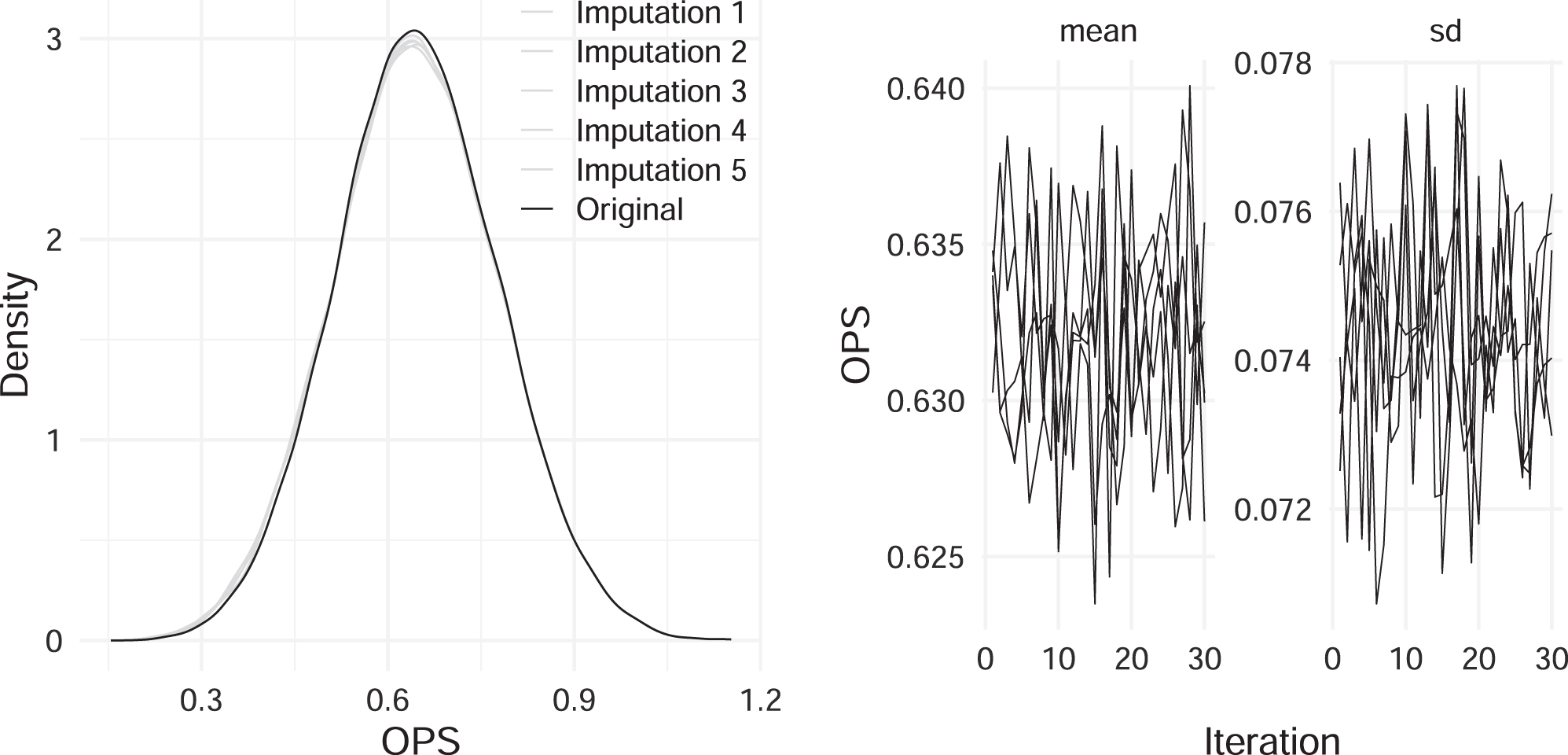
Additionally, we perform diagnostics to assess the plausibility of the imputations, and also examine whether the MICE algorithm converges. We first check for distributional discrepancy by comparing the distributions of the fully observed and imputed data. Figure 3 (left) presents the density curves of the OPS values for each imputed dataset and the fully simulated data. It is obvious that the imputation distributions are well-matched with the observed data. To confirm convergence of the MICE algorithm, we inspect trace plots for the mean and standard deviation of the imputed OPS values. As shown in Fig. 3 (right), convergence is apparent, since no definite trend is revealed and the imputation chains are intermingled with one another.
Fig. 3
Left: Kernel density estimates for the fully observed and imputed OPS values. Right: Trace plots for the mean and standard deviation of the imputed OPS values against the iteration number for the imputed data. Results shown here are for the dropout case of players having OPS average from age 21 to 25 below 0.55.
5Application: MLB data
Lastly, we apply the previously mentioned multilevel multiple imputation model to estimate the average OPS aging curve for MLB players. For this investigation, besides the data pre-processing tasks mentioned in Section 3.1, our sample is limited to all players who made their major league debut no sooner than 1985, resulting in a total of 2323 players. To perform imputation, we pass in the same parameters to our simulation study (m = 5 with 30 iterations for each imputation).
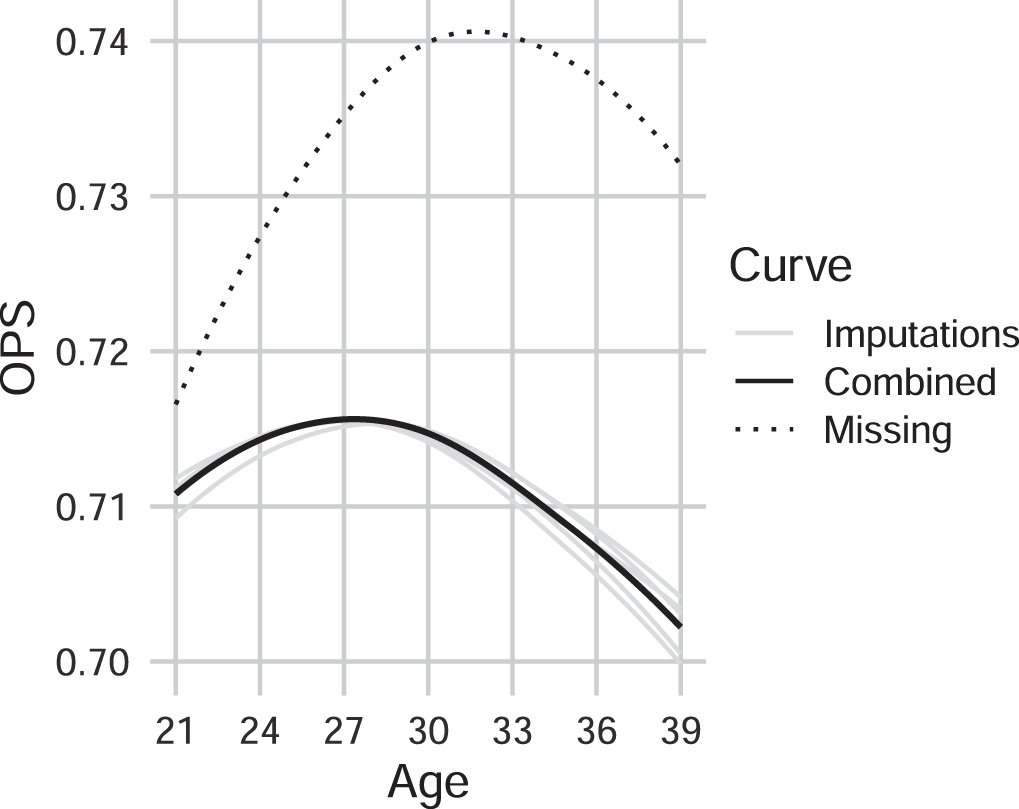
Figure 4 shows the OPS aging curves for MLB players estimated with and without imputation. The plot illustrates a similar result as our simulations as the combined curve based on imputations is lower than the curve obtained when ignoring the missing data. The peak age after imputation occurs much earlier (26 years old) compared to the peak age when player dropout is not accounted for (30 years old). It is clear that the aging effect is overestimated without considering the unobserved player-seasons. In other words, the actual performance declines with age more rapidly than estimates based on only the observed data.
Fig. 4
Comparison of the average OPS aging curves constructed with only observed players and imputation for MLB data. Note that the “Missing” curve is obtained when the missing data (unobserved player seasons) are ignored. Results shown here are for 2,323 players who made their MLB debut in or after 1985.
6Discussion
The concept of survival bias is frequently seen in professional sports, and our paper approaches the topic of aging curves and player dropout in baseball as a missing data problem. We use multiple imputation with a multilevel structure to improve estimates for the aging curves. Through simulation, we highlight that ignoring the missing seasons leads to an overestimation of the age effect on baseball offensive performance. With imputation, we achieve an aging curve showing that players actually decline faster as they get older than previously estimated.
There are notable limitations of our study which leave room for improvement in future work. In our current imputation model, age is the only predictor for estimating performance. It is possible to include more covariates in the imputation algorithm and determine whether a better aging curve estimate is achieved. In particular, we can factor in other baseball offensive statistics (e.g., home run rate, strikeout rate, WOBA, walk rate, etc.) in building an imputation model for OPS. We can also examine other performance metrics to see how age affects different statistics.
Furthermore, the aging curve estimation problem can be investigated in a completely different statistical setting. As noted in Section 2, rather than considering discrete observations, another way of studying aging curves is through a continuous approach, assuming a smooth curve for career performance. As pointed out by Wakim & Jin (2014), methods such as functional data analysis (FDA) and principal components analysis through conditional expectation (PACE) possess many modeling advantages, in regard to flexibility and robustness. There exists a number of proposed multiple imputation algorithms for functional data (He et al. 2011, Ciarleglio et al. 2021, Rao & Reimherr 2021), which all can be applied in future studies on aging curves in sports.
Acknowledgments
We thank the organizers of the 2022 Carnegie Mellon Sports Analytics Conference (CMSAC) for the opportunity to present this work and receive feedback. We thank the anonymous reviewers of the Reproducible Research Competition at CMSAC 2022 for the insightful comments and suggestions. We thank Kathryne Piazza for her help in the early stages of this project.
Supplementary material
[1] All code related to this paper is available athttps://github.com/qntkhvn/aging.
References
1 | Albert J. , (1992) , ‘A bayesian analysis of a poisson random effects model for home run hitters’, The American Statistician 46: (4), 246. |
2 | Albert J. , (1999) , ‘Bridging different eras in sports: Comment’, Journal of the American Statistical Association 94: (447), 677. |
3 | Albert J. , 2002, ‘Smoothing career trajectories of baseball hitters’, Unpublished manuscript, Bowling Green State University. URL: https://bayesball.github.io/papers/career trajectory.pdf |
4 | Bates D. , Mächler M. , Bolker B. , Walker S. M. , (2015) , ‘Fitting linear mixed-effects models using lme’, Journal of Statistical Software 67: (1), 1–48. |
5 | Berry S. M. , Reese C. S. , Larkey J. C. (1999) , ‘Bridging different eras in sports’, Journal of the American Statistical Association 661–676. |
6 | Bradbury J. C. (2009) , ‘Peak athletic performance and ageing: Evidence from baseball’, Journal of Sports Sciences 27: (6), 599–610. |
7 | Brander J. A. , Egan E. J. , Yeung L. (2014) , ‘Estimating the effects of age on NHL player performance’, Journal of Quantitative Analysis in Sports 10: (2). |
8 | Ciarleglio A. , Petkova E. , Harel O. (2021) , ‘Elucidating age and sex-dependent association between frontal EEG asymmetry and depression: An application of multiple imputation in functional regression’, Journal of the American Statistical Association 117: (537), 12–26. |
9 | Dendir S. (2016) , ‘When do soccer players peak? A note’, Journal of Sports Analytics 2: (2), 89–105. |
10 | Fair R. C. (1994) , ‘How Fast Do Old Men Slow Down?’, The Review of Economics and Statistics 76: (1), 103–118. |
11 | Fair R. C. (2007) , ‘Estimated age effects in athletic events and chess’, Experimental Aging Research 33: (1), 37–57. |
12 | Fair R. C. (2008) , ‘Estimated age effects in baseball’, Journal of Quantitative Analysis in Sports 4: (1). |
13 | Friendly M. , Dalzell C. , Monkman M , Murphy D. ,2022, Lahman:Sean ‘Lahman’ Baseball Database. R package version 10.0-1. URL: https://CRAN.R-project.org/package=Lahman |
14 | Gelman A. , Hill J ,2006, Data Analysis Using Regression and Multilevel/Hierarchical Models, Cambridge University Press. |
15 | He Y. , Yucel R. , Raghunathan T. E. (2011) , ‘A functional multiple imputation approach to incomplete longitudinal data’, Statistics in Medicine 30: (10), 1137–1156. |
16 | Judge J. ,2020a, ‘An approach to survivor bias in baseball’, BaseballProspectus.com. Accessed 27-Jul-2022. URL: https://www.baseballprospectus.com/news/article/59491/anapproach-to-survivor-bias-inbaseball |
17 | Judge J. b ,2020b, ‘The Delta Method, Revisited: Rethinking Aging Curves’, BaseballProspectus.com. Accessed 27-July-2022. URL: https://www.baseballprospectus.com/news/article/59972/the-delta-method-revisited |
18 | Kasim R. M. , Raudenbush S. W. (1998) , ‘Application of gibbs sampling to nested variance components models with heterogeneous within-group variance’, Journal of Educational and Behavioral Statistics 23: (2), 93–116. |
19 | Kovalchik S. A. (2014) , ‘The older they rise the younger they fall: age and performance trends in men’s professional tennis from 1991 to 2012’, Journal of Quantitative Analysis in Sports 10: (2). |
20 | Lahman S. ,2021, ‘Lahman’s baseball database’, SeanLahman. com. URL: https://www.seanlahman.com/baseballarchive/statistics/ |
21 | Lailvaux S. P. , Wilson R. , Kasumovic M. M. (2014) , ‘Trait compensation and sex-specific aging of performance in male and female professional basketball players’, Evolution 68: (5), 1523–1532. |
22 | Leroy A. , Marc A. , Dupas O. , Rey M. , Lichtman J. L. , Gey S. (2018) , ‘Functional Data Analysis in Sport Science: Example of Swimmers’ Progression Curves Clustering’, Applied Sciences 8: (10), 1766. |
23 | Lichtman M. , ‘How do baseball players age? (part 2)’, The Hardball Times. Accessed 1-August-2022. URL: https://tht.fangraphs.com/how-do-baseball-players-age-part-2 |
24 | Little R. J. A. , Rubin D. B. ,1987, Statistical AnalysisWith Missing Data, Wiley Series in Probability and Statistics, Wiley. |
25 | Marchi M. , Albert J. , Baumer B. S. ,2018, Analyzing baseball data with R, 2 edn, Boca Raton, FL: Chapman and Hall/CRC Press. |
26 | Morris D. H. , ‘A study of age group track and field records to relate age and running speed’253: (5489), 264–265. |
27 | Morris C. N. (1983) , ‘Parametric empirical bayes inference: Theory and applications’, Journal of the American Statistical 78: (381), 47–55. |
28 | Page G. L. , Barney B. J. , McGuire A. T. (2013) , ‘Effect of position, usage rate, and per game minutes played on NBA player production curves’, Journal of Quantitative Analysis in Sports 9: (4), 337–345. |
29 | R Core Team 2023, R: A Language and Environment for Statistical Computing, R Foundation for Statistical Computing, Vienna, Austria. URL:https://www.R-project.org/ |
30 | Rao A. R. , Reimherr M. (2021) , ‘Modern multiple imputation with functional data’, Stat 10: (1). |
31 | Rubin D. B. (1976) ,‘Inference and missing data’, Biometrika 63: (3), 581–592. |
32 | Rubin D. B. ,1987, Multiple Imputation for Nonresponse in Surveys, John Wiley & Sons, Inc. |
33 | Säfvenberg R. ,2022, Age of peak performance among swedish football players, Master’s thesis, Linköping University, The Division of Statistics and Machine Learning. URL: https://www.diva-portal.org/smash/get/diva2:1674221/FULLTEXT01.pdf |
34 | Schell T. , Smith G. (2000) , ‘Career trajectories in baseball’, CHANCE 13: (4), 35–38. |
35 | Schell M. J ,2005, Calling It a Career: Examining Player Aging, Princeton University Press, pp. 45-57. |
36 | Schuckers M. , Lopez M. , Macdonald B. ,2023, ‘Estimation of player aging curves using regression and imputation’, Annals of Operations Research |
37 | Schulz R. , Curnow C. (1988) , ‘Peak performance and age among superathletes: Track and field, swimming, baseball, tennis, and golf’, Journal of Gerontology 43: (5), 113–120. |
38 | Schulz R. , Musa D. , Staszewski J. , Siegler R. S. , (1994) ,‘The relationship between age and major league baseball performance: Implications for development,’, Psychology and Aging 9: (2), 274–286. |
39 | Stival M. , Bernardi M. , Cattelan M. , Dellaportas P. (2023) , ‘Missing data patterns in runners’ careers: do they matter?’, Journal of the Royal Statistical Society Series C: Applied Statistics 72: (2) 213–230 . |
40 | Turtoro C. , ‘Flexible aging in the nhl using gam’, RPubs. Accessed 1-August-2022. URL:https://rpubs.com/cjtdevil/nhlaging |
41 | Vaci N. , Cocić D. , Gula B. , Bilalić M. (2019) , ‘Large data and bayesian modeling—aging curves of NBA players’, Behavior Research Methods 51: (4), 1544–1564. |
42 | van Buuren S. , Groothuis-Oudshoorn K. 1999,Flexible Multivariate Imputation by MICE, Vol. PG/VGZ/99.054, Leiden: TNO Prevention; Health. |
43 | van Buuren S. , Groothuis-Oudshoorn K. (2011) , ‘mice: Multivariate imputation by chained equations in R’, Journal of Statistical Software 45: (3), 1–67. |
44 | Villaroel C. , Mora R. , Parra G. C. G. , 2011, ‘Elite triathlete performance related to age’Journal of Human Sport and Exercise 6(2 (Suppl.)), 363-373. |
45 | Wakim A. , Jin J. , 2014, ‘Functional data analysis of aging curves in sports‘, arXiv preprint arXiv:1403.7548. |

