
Enhancement of digital radiography image quality using a convolutional neural network
Abstract
Digital radiography system is widely used for noninvasive security check and medical imaging examination. However, the system has a limitation of lower image quality in spatial resolution and signal to noise ratio. In this study, we explored whether the image quality acquired by the digital radiography system can be improved with a modified convolutional neural network to generate high-resolution images with reduced noise from the original low-quality images. The experiment evaluated on a test dataset, which contains 5 X-ray images, showed that the proposed method outperformed the traditional methods (i.e., bicubic interpolation and 3D block-matching approach) as measured by peak signal to noise ratio (PSNR) about 1.3 dB while kept highly efficient processing time within one second. Experimental results demonstrated that a residual to residual (RTR) convolutional neural network remarkably improved the image quality of object structural details by increasing the image resolution and reducing image noise. Thus, this study indicated that applying this RTR convolutional neural network system was useful to improve image quality acquired by the digital radiography system.
1Introduction
X-ray digital radiography (DR) is an essential method for non-destructive detection in security check and medical imaging examination, which can show internal details and structures of objects. However, limited by the costs and the techniques, the images acquired by the digital radiography system usually have low spatial resolution and a significant amount of noise. As a result, the images are often too blurry to reveal the details of the region of interest (ROI). Thus, it is highly desirable to improve image resolution and eliminate image noise to restore the image details.
The problem is resulted from single image super resolution (SISR) and x-ray image denoising. The SISR is a classical ill-posed and inverse problem in image processing, which may enhance the image quality and overcoming the resolution limitations of the acquired image data. The noises in x-ray images are non-Gaussian, spatial-variant and related to surrounding structures which are hard to eliminate while maintaining the surrounding details. It is difficult to solve these problems with conventional methods due to the inherent physical limitations.
More recently, deep learning methods, especially deep convolution neural networks (CNNs), have achieved impressive success in various computer vision tasks, ranging from segmentation, detection and recognition [1–3]. It has also been applied in X-ray imaging for variety of applications [4, 5]. Meanwhile, deep learning based methods have been applied to low-level computer vision applications such as denoising and super-resolution, which have been extensively investigated with great performance [6–8]. Although great achievement have been made, most of the existing CNN based x-ray image denoising models suffer gradient exploding/vanishing problem as networks go deeper. Furthermore, the number of network parameters, which has great influence on performance and speed, is not taken into account in most CNN based methods.
In this study, we employed a modified neural network to solve the problems of x-ray image super-resolution and denoising. In order to alleviate the gradient exploding/vanishing problem, we used a skip connection method in the CNN model. Meanwhile, a deconvolution layer is introduced to the model to improve the image resolution and restore the image details. In particular, we added a residual image from the low-resolution image and its corresponding coarse image as an input for the neural network, which is helpful for the model to extrapolate the image and reduce the noise.
2Related works
2.1Image super resolution
Limited by the imaging system, low-resolution image contains less information than a high-resolution image. However, different from random signal, image features are locally correlative to spatial domain, which indicates the possibility to restore the missing pixels from the neighboring pixels. Image super-resolution can detect the mapping function from high-resolution (HR) images to low-resolution (LR) images.
Image SR can be categorized into two main types of approaches: interpolation-based, and learning- based methods. Interpolation-based methods generate HR pixel values by using weighted average of neighboring LR pixel values (bicubic, Lanczos) [9]. While the interpolation-based method generates smooth regions, the high frequency details (texture and edge) can’t be restored well. Using extracted image features from external images, learning-based methods formulate the mapping function from LR image to HR image, which is learned in a supervised manner. Extracting the image priors from external data, the learning-based method has shown great potential in super resolution [10–12].
Recently, the deep learning methods, especially deep convolution neural networks (CNNs), have been widely used in various computer vision tasks with great success. A recent study adopted the convolution neural network to solve the SISR problem and achieved state-of-the-art performance [13]. The proposed net comprises three layers corresponding to patch extraction, non-linear mapping and reconstruction, which are also processed in sparse code methods. Then, Wang and colleagues [14] combined the sparse representation with deep network. Similarly, Gu et al. [15] applied the sparse coding to the entire image instead of overlapping patches done by previous works. Dong et al. [16] used a method in which deconvolution layer is adopted to upscale the image in the last layer of the network, which further increased performance in terms of both accuracy and speed. Kim et al. proposed a very deep CNN (VDSR) with over 20 layers to predict the residual between the HR and LR images, which observably boosts the convergence speed and performance [17].
2.2Image denoising
As one of the classical problems in image processing, image denoising problem has attracted continuous attention for several decades. Estimating the denoised patch instead of estimating each pixel separately, Dabov et al. proposed the BM3D algorithm that employs non-local similar patches for denoising image patches [18]. Considering the denoising as a kind of low-rank matrix approximation problem, Gu et al. proposed a weighted nuclear norm minimization (WNNM) to solve the problem [19].By extracting the image priors and learning the mapping function from noisy images to less noisy ones in the training datasets, deep learning based denoising methods achieved much higher performance than traditional denoiser. Most recently, Ahn and Cho proposed a block-matching convolutional neural network (BMCNN) that combines the BM3D and CNN, and achieved state-of-the-art performance [20]. Recent studies have provided promising results by applying CNN based denoisers to X-ray images [21, 22]. The CNNs are trained from normal-dose images and their corresponding low-dose images generated by adding Poisson noises based on physical models. Kang et al. proposed a wavenet method which combines a deep convolution neural network with a directional wavelet transform and achieved much better performance [22].
2.3Convolution neural networks
Convolution neural network, suitable for image processing, has shown great performance in image classification and is gaining popularity in other computer vision fields. The classical CNN is composed of convolutional layer, batch normalization layer and activation layer. The composition of convolutional layer and non-linearity layer can written as
(1)
To solve the vanishing/exploding gradient problem, the residual blocks and skip-connections introduced by He and colleagues [24] was adopted to ease the training of deep CNNs, which reformulate the deep layer to predict the residual information. The structure makes it possible to train a very deep CNN and achieve amazing performance.
3Proposed method
3.1Proposed network
In this study, we propose a residual to residual network (RTR) based on a cascade of convolutional neural networks (CNNs). The architecture of the network is outlined in Fig. 1, which consists of three parts: a deep CNN of low-quality image, a CNN of residual image and a bicubic interpolation operation.
Fig.1
Network architecture of the proposed RTR method.
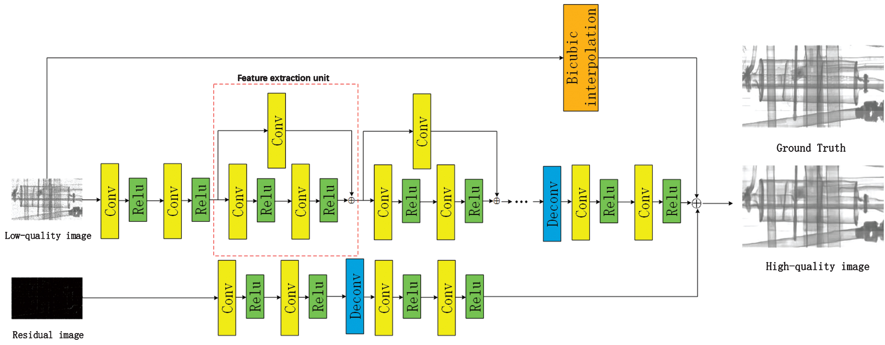
The bicubic image contains the same low-frequency information with high-quality image, while the deep CNN is set to learn the residual image with high-frequency details, which aims at easing the training process. Since the low-quality can be regarded as a degrading result of a high-quality image. The coarse image is also a degrading result of the low-quality image, which can be obtained by two steps: sub-sampling the low-quality image and adding noise, then up-sampling the result to the same size of low-quality image by interpolation. The residual image is the difference between the low-quality image and its corresponding coarse image. Containing the self-similarity information, the residual image can be taken as input of a CNN, which could predict the residual of high-quality image and low-quality image. Furthermore, the deep CNN of low-quality image is composed of three modules: feature extraction, up-sampling and reconstruction. We will detail the architectures and functions of each module in deep CNN later.
3.1.1Feature extraction
Most of the previous learning based methods extract the image features using filters artificially designed or learned by a shallow net and cannot sufficiently extract the image details. As evaluated previously by He and colleagues [24], the residual blocks with short connections can effectively facilitate gradients flow through multiple layers, thus easing the training process of the deep network. To solve the problem, the proposed method uses a structure with cascading feature extraction units. Inspired by the Resnet from He and colleagues [24], the feature extraction unit consists of two cascading convolution layers with skip connections to decrease the difficulty of training, thus the network has stronger capacity to extract the image features. Furthermore, a convolution layer is set to the skip connection without activation function, which may reserve the information of previous layer and improve the representation power. The convolution layers are activated by Rectified Linear Unites (ReLUs) acting as nonlinear mappings. Each convolution layer can be expressed as
(2)
3.1.2Up-sampling
The up-sampling operation is performed by a deconvolution layer, which upscales the previous features extracted by cascading convolution layers. The deconvolution can be regarded as an inverse operation of convolution, in which filters are also learned from input features. For the stride k, the spatial size of the output feature maps is upscaled to k times of the input by reversing the forward and backward propagation of convolution layers. For the image SR problem, the stride k determines the upscaling factor.
The performance of different filter size of the deconvolution layer was described in the previous study [16]. The proposed method uses a smaller filter size of the deconvolution is five. The output of the up-sampling module is an upscaled image, thus the number of filters is set to be one. Meanwhile, zero padding is adopted to preserve the spatial size of the upscaled image. Different from upscaling the images by interpolation method, the filters of deconvolution layer are learned from the training dataset, which are meaningful and suitable for image SR.
3.1.3Reconstruction
Directly generated by feature maps with small size, the output of the up-sampling module contains less information than a high-quality image. To further increase the performance, two convolution layers are introduced after the deconvolution layer to restore the high-quality image with the context information of the upscaled image. For both effectiveness and efficiency, the convolution layers adopt filter size 3 and the number of filters is set to be 16. The output feature map of the last convolution layer combines the low-frequency information of bicubic image and reconstruct the final high-quality images.
3.1.4Summary
Compared to previous CNN based method, the improvements of proposed RTR are described below:
1. The introduction of internal connections allows us to adopt a deeper network which can obtain larger image regions with more information for reconstruction.
2. The deep network is designed to predict the residual images with high-frequency details while the low-frequency information is contained in bicubic image, which significantly boost convergence of the training process.
3. Adopting the residual image as input, the proposed method adds the self-similarity information of image in the network and further improves the performance.
3.2Training
The aim of image super resolution is to generate an image as similar as possible to the ground truth high-quality image. So given N training image pairs
(3)
The training process is conducted by the mini-batch stochastic gradient descent method with a batch size of 64, momentum of 0.9, while all the filters of convolution layers are randomly initialized from a zero-mean Gaussian distribution with standard deviation 0.01. To get the stable filters efficiently, adjustable Gradient Clipping is used, the learning rate is initially set to 0.1 and decreased by a factor of 0.1 until the validation loss is stabilized.
The proposed model is trained using the Caffe package on a workstation with an Intel i7 6800k CPU and a GTX1080 GPU.
4Experiments
4.1Dataset
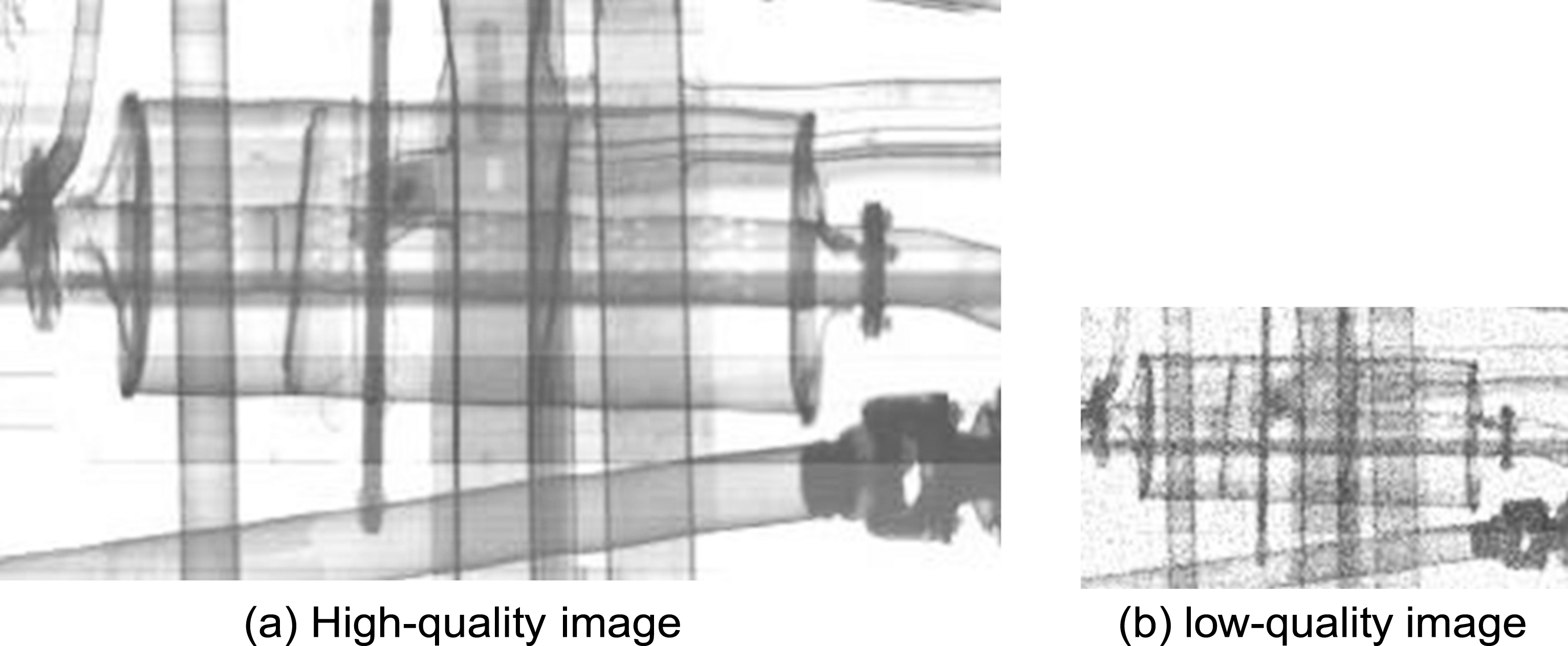
Dong and colleagues [13] reported that the effect of big data in low-level computer vision problems is not as impressive as that shown in high-level computer vision problems. So 80 images acquired by the digital radiography system were used as a training dataset for the experiments, which is sufficient for the task. It contained DR images collected from 3 different cars with a 450kev X-ray machines and 1984 2.5 mm * 2.5 mm scintillation detector elements. The corresponding low-quality images were simulated by reducing size and adding Poisson noises to each high-quality images. To avoid over-fitting and make full use of the dataset, data augmentation techniques including rotation and flipping are used, which generates 5 times more images for training. Figure 2 shows a typical image of the dataset, while Fig. 3 shows an original ROI image and its corresponding low-quality image.
Fig.2
An example image of the dataset.
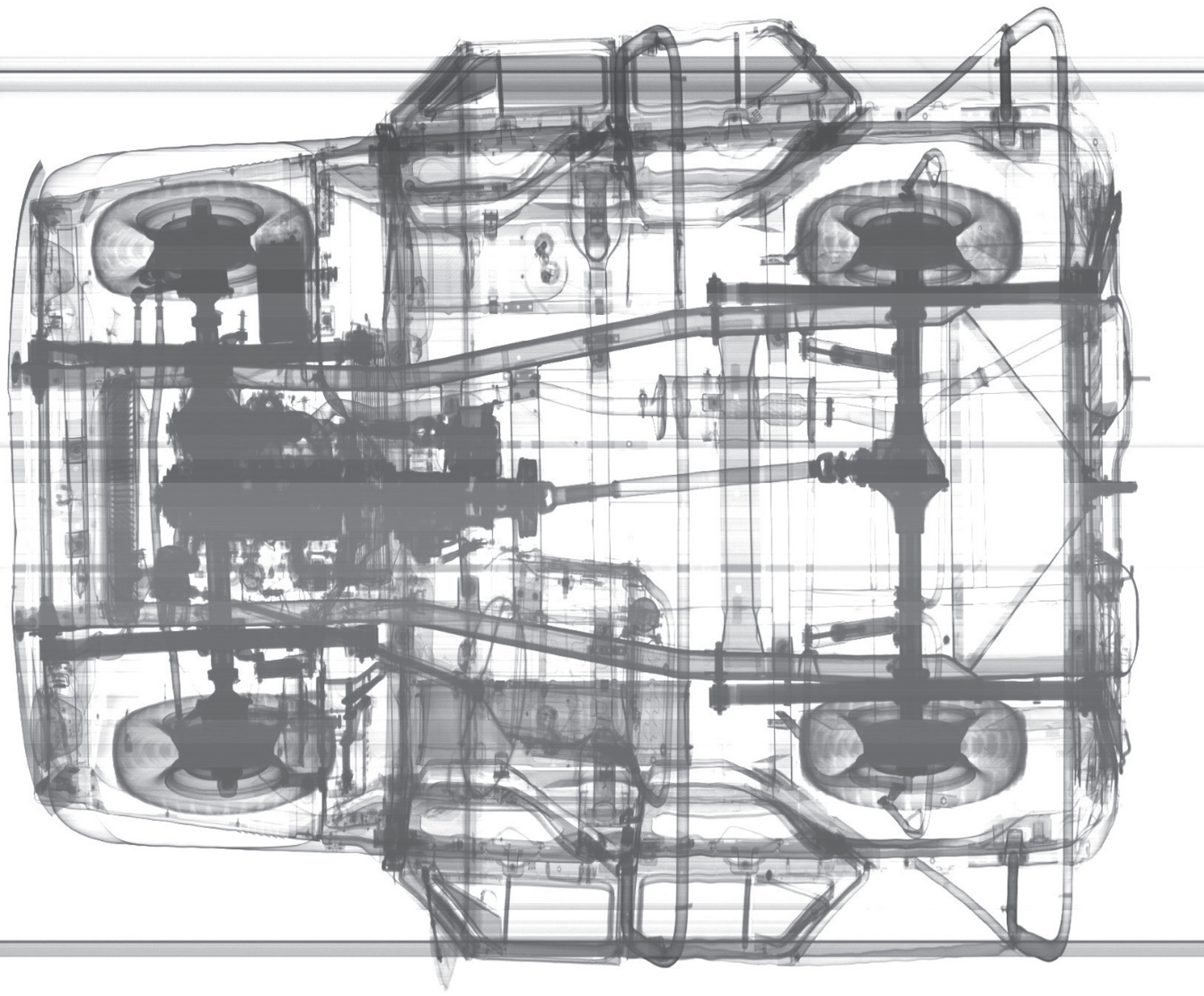
Fig.3
High-quality image and its corresponding low-quality image.
Since direct processing of the entire DR image is impractical, the training images are randomly cropped to patches as the ground truth HR examples, which are proportional to depth of RTR network. The size of the patches can be calculated as:
(4)
It should be noted that the training dataset used in this study is quite different from real application. A better choice is to take a more practical way to generate the training data in real applications. For example, we can choose images with longer exposure time and less statistical noises as ground truth images while images with shorter exposure time and more statistical noises can be set as input images.
4.2Architecture analysis
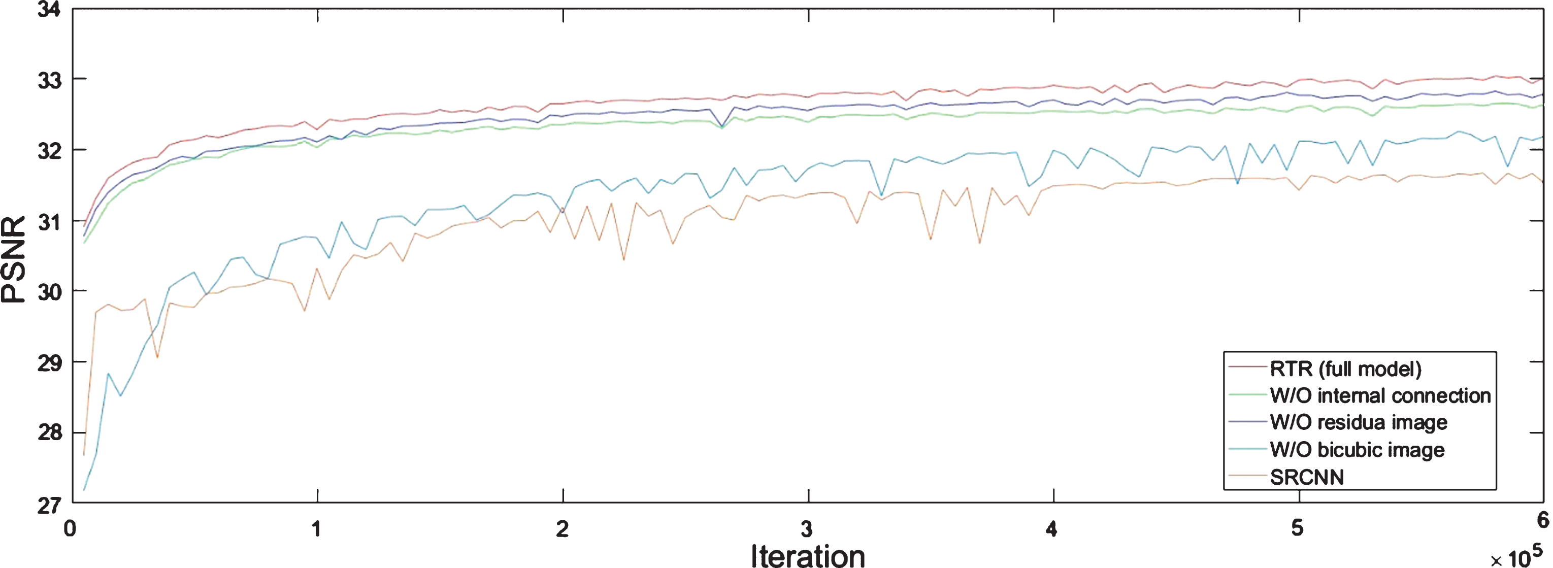
To prove the efficiency of the network of the proposed method, the proposed method and its variants are evaluated on a test dataset with 5 images acquired from the same system with the training dataset. PSNR metrics are used for quantitative evaluation, which are widely used in image denoising and SR problem. To investigate the impact of the introduction of each module on the final performance, we trained the proposed network and its variant without bicubic interpolation image, without residual image and without internal connection in feature extraction unit respectively. The experiment strictly followed the above implementation details, and the upscaling factor of the network is set to be 2. The number of filters of each convolution layer is set to 16, and the number of the feature extraction unit is set to 4. To validate the proposed method, the SRCNN is also trained on the dataset. Figure 4 depicts the PSNR convergence curves of the networks on the test set.
Fig.4
Performance curves for different networks on the test dataset with an up-sampling factor 2.
4.2.1Bicubic interpolation image
Our method introduces a bicubic image and trains the deep net to predict the residual image. As the figure shows, the network with bicubic image converges much faster and shows better performance than the network without bicubic image, which also can be observed in deep residual net. From the experimental results, we could conclude that the introduction of the bicubic image plays a similar role as the short connections in the deep residual net, which set the deep net to learn the residual image and eases the training process of network.
4.2.2Residual image
We add a residual image of the low-resolution image and its corresponding coarse image as an input of the neural network. As the figure shows, the network with residual image shows better performance than the network without residual image, which also can be observed in deep residual net. From the experimental results, we could conclude that the image self-similarity is incorporated into the RTR network to predict the target residual image, which improves the performance of the network.
4.2.3Internal connections
As evaluated in deep residual net, skip connection is helpful to ease training and improve the performance, which has been widely used to train deep CNNs. In this study, we introduce internal connections in the feature unit. Meanwhile, we adopt a convolution layer without activation function to avoid loss of the information from the previous layer caused by Relu layers. The results show that the internal connections is an essential structure for the RTR network, which leads to a performance improvement.
5Results
5.1Performance differences of using more or less parameters
The reconstruction performance can be improved by adopting more parameters at the cost of running time. A suitable parameter number selection would accelerate the reconstruction while maintaining a good performance. The RTR network consists of M convolution layers and a deconvolution layer and the filter number of each layer is N. Due to the filter size of each convolution layer is set to 3. The parameter number can be calculated as
(5)
As a result, width and depth are two sensitive variables which decides the parameter number of the network. To evaluate the relationship performance and parameter numbers, different depth and width of RTR were tested in this study. Different settings are named as RTR-d-w, where d is the number of feature extract units and w is the number of filters. In this study, RTR-1-16, RTR-1-32, RTR-1-64, RTR-2-16, RTR-2-32, RTR-2-64, RTR-4-16, RTR-4-32, and RTR-4-64 are tested on a 128*128 ROI image. The results of RTR with different depth and width are shown in the Table 1. From the table, we can observe that both the increase of width and depth improve the performance. However, RTR-4-32 get better performance with less parameters and time consuming than RTR-1-64 and RTR-2-64, which indicates that the increase of the depth of the network is a more effective way to improve the performance. Although most of image denoising network adopt 64 filters for each convolution layer, the performance difference between RTR-4-32 and RTR-4-64 is not remarkable, which indicates that the parameters of RTR-4-32 is sufficient for the dataset to represent the image features. The running times of processing the ROI image of the RTR are in one second, however it’s still time consuming for RTR to process a large x-ray image. Thus, RTR-4-16 is recommended to balance the processing speed and performance on this dataset, while different options should be tested on different datasets.
Table 1
Average PSNR and test time comparison on test dataset of different methods
| Method | RTR-1-16 | RTR-1-32 | RTR-1-64 | RTR-2-16 | RTR-2-32 | RTR-2-64 | RTR-4-16 | RTR-4-32 | RTR-4-64 |
| Parameters | 13184 | 49408 | 190976 | 20096 | 77056 | 301568 | 33920 | 132352 | 552752 |
| Time (s) | 0.10 | 0.24 | 0.62 | 0.14 | 0.33 | 0.83 | 0.21 | 0.53 | 1.02 |
| PSNR (db) | 30.43 | 30.63 | 30.71 | 30.67 | 30.84 | 30.91 | 30.79 | 30.95 | 30.98 |
5.2Comparison with conventional methods
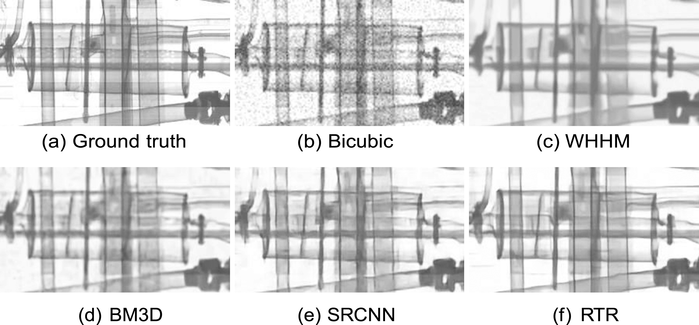
The experimental results with the proposed RTR method clearly differ from those with other methods, namely the Bicubic, WNNM, BM3D and SRCNN. In the test, the upscale factor of the low-quality image is 2, and the WNNM and BM3D are operated on the bicubic image, while SRCNN is trained on the same dataset with RTR. Table 2 summarizes the quantitative performance (PSNR and test time) for different upscaling factors. The proposed RTR method outperforms the previous methods on the PSNR values. It is shown that larger data is beneficial to the final performance, thus further performance improvements of our method can also be expected when using more training images. Figures 5–7 show the enhanced images processed by different methods. The high-quality images generated by the proposed RTR method are much clearer than other results with sharper edges and less artifacts.
Table 2
PSNR comparison on three ROI images with different methods
| Method | Bicubic | WHHM | BM3D | SRCNN | RTR |
| ROI1 | 26.09 | 27.95 | 28.05 | 29.06 | 30.08 |
| ROI2 | 26.99 | 29.65 | 29.78 | 29.87 | 30.77 |
| ROI3 | 28.45 | 31.57 | 31.76 | 31.65 | 32.45 |
| Mean | 27.18 | 29.72 | 29.86 | 30.20 | 31.11 |
Fig.5
Enhancing results of ROI1 with upscaling factor 2.
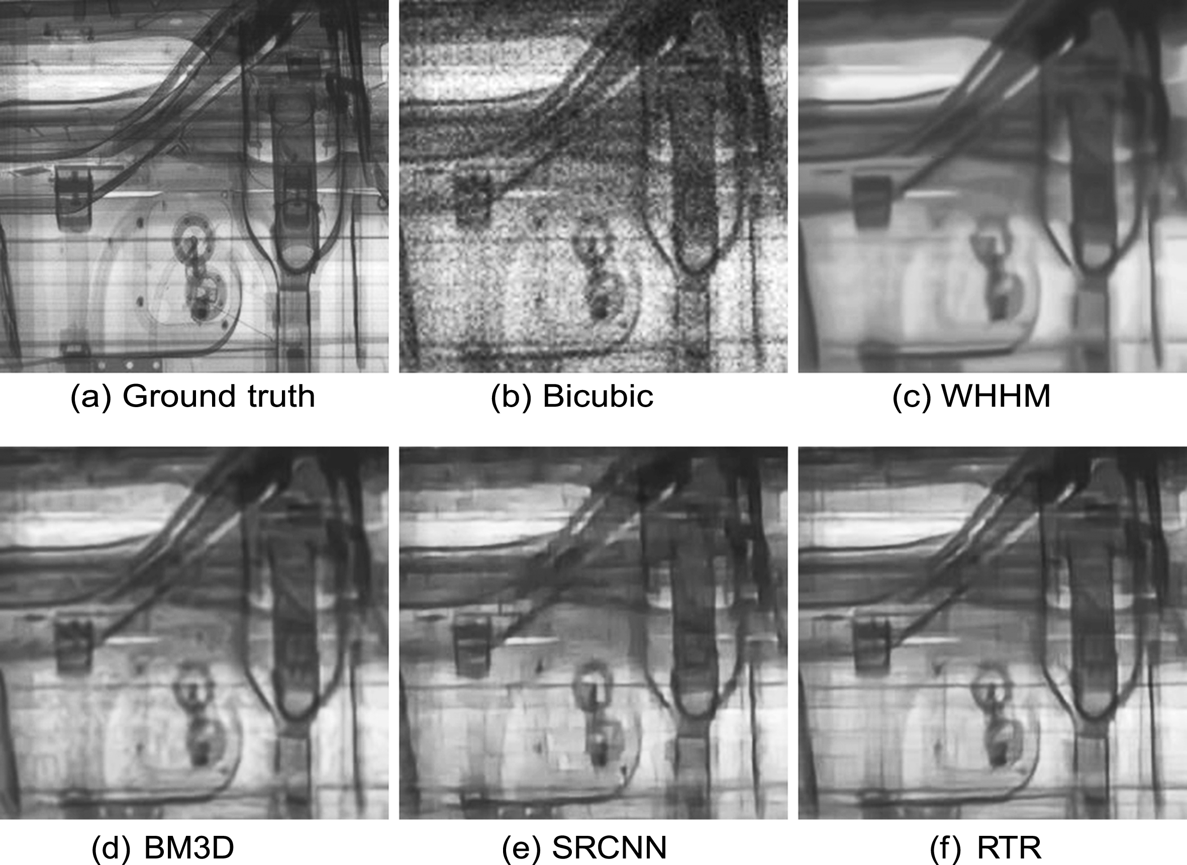
Fig.6
Enhancing results of ROI2 with upscaling factor 2.
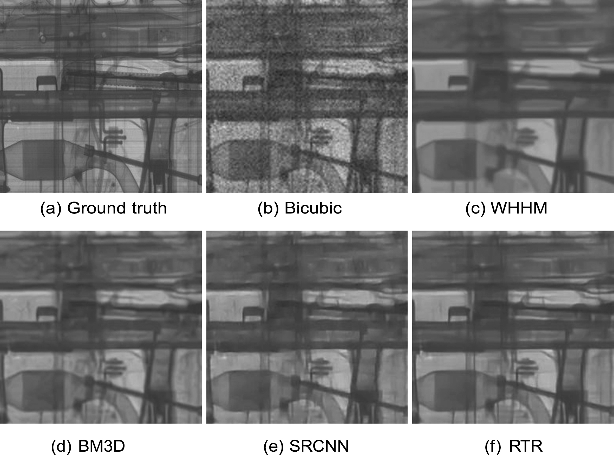
Fig.7
Enhancing results of ROI3 with upscaling factor 2.
6Conclusions
In this study, a residual to residual CNN method has been proposed and tested to enhance low-quality DR image with increased image resolution and signal-to-noise ratio (denoising). The RTR network incorporates the image self-similarity by adding the residual image from the input image and its coarse image as an input. Study results showed that the proposed method effectively suppressed the noise and enhanced DR image quality, which indicates a great potential for applying deep learning to DR image processing. In addition, study has also demonstrated that selecting an appropriate number of parameters could boost the processing speed while maintaining excellent performance.
Acknowledgments
This work is supported by the Beijing Key Laboratory of Nuclear Detection.
References
[1] | He K. , Zhang X. , Ren S. , Sun J. , Spatial pyramid pooling in deep convolutional networks for visual recognition, in: European Conference on Computer Vision, Springer; (2014) , pp. 346–361. |
[2] | Zhang N. , Donahue J. , Girshick R. , Darrell T. , Part-based r-cnns for fine-grained category detection, in: European conference on computer vision, Springer; (2014) , pp. 834–849. |
[3] | Sermanet P. , Eigen D. , Zhang X. , Mathieu M. , Fergus R. and LeCun Y. , Overfeat: Integrated recognition, localization and detection using convolutional networks, arXiv preprint arXiv:1312.6229. |
[4] | Jaccard N. , Rogers T.W. , Morton E.J. and Griffin L.D. , Detection of concealed cars in complex cargo X-ray imagery using deep learning, Journal of X-ray Science and Technology 25: (3) ((2017) ), 323–339. |
[5] | Wang Y. , Qiu Y. , Thai T. , Moore K. , Liu H. and Zheng B. , A two-step convolutional neural network based computer-aided detection scheme for automatically segmenting adipose tissue depicting on CT images, Computer Methods and Programs in Biomedicine 144: ((2017) ), 97–104. |
[6] | Xie J. , Xu L. , Chen E. , Image denoising and inpainting with deep neural networks, in: Advances in Neural Information Processing Systems, (2012) , pp. 341–349. |
[7] | Zhang K. , Zuo W. , Chen Y. , Meng D. and Zhang L. , Beyond a gaussian denoiser: Residual learning of deep cnn for image denoising, IEEE Transactions on Image Processing 26: (7) ((2017) ), 3142–3155. |
[8] | Dong C. , Loy C.C. , He K. , Tang X. , Learning a deep convolutional network for image super- resolution, in: European Conference on Computer Vision, Springer; (2014) , pp. 184–199. |
[9] | Keys R. , Cubic convolution interpolation for digital image processing, IEEE Transactions on Acoustics, Speech, and Signal Processing 29: (6) ((1981) ), 1153–1160. |
[10] | Yang J. , Wright J. , Huang T.S. and Ma Y. , Image super-resolution via sparse representation, IEEE Transactions on Image Processing 19: (11) ((2010) ), 2861–2873. |
[11] | Timofte R. , De Smet V. and Van Gool L., Anchored neighborhood regression for fast example- based super-resolution, in: Proceedings of the IEEE International Conference on Computer Vision, (2013) , pp. 1920–1927. |
[12] | Timofte R. , De Smet V. and Van Gool L., A+: Adjusted anchored neighborhood regression for fast super-resolution, in: Asian Conference on Computer Vision, Springer; (2014) , pp. 111–126. |
[13] | Dong C. , Loy C.C. , He K. and Tang X. , Image super-resolution using deep convolutional networks, IEEE Transactions on Pattern Analysis and Machine Intelligence 38: (2) ((2016) ), 295–307. |
[14] | Wang Z. , Liu D. , Yang J. , Han W. and Huang T. , Deep networks for image super-resolution with sparse prior, in: Proceedings of the IEEE International Conference on Computer Vision, (2015) , pp. 370–378. |
[15] | Gu S. , Zuo W. , Xie Q. , Meng D. , Feng X. and Zhang L. , Convolutional sparse coding for image super-resolution, in: Proceedings of the IEEE International Conference on Computer Vision, (2015) , pp. 1823–1831. |
[16] | Dong C. , Loy C.C. and Tang X. , Accelerating the super-resolution convolutional neural network, in: European Conference on Computer Vision, Springer; (2016) , pp. 391–407. |
[17] | Kim J. , Kwon Lee J. and Mu Lee K., Accurate image super-resolution using very deep convolutional networks, in: Proceedings of the IEEE Conference on Computer Vision and Pattern Recognition, (2016) , pp. 1646–1654. |
[18] | Dabov K. , Foi A. , Katkovnik V. and Egiazarian K. , Image denoising by sparse 3-d transform-domain collaborative filtering, IEEE Transactions on Image Processing 16: (8) ((2007) ), 2080–2095. |
[19] | Gu S. , Zhang L. , Zuo W. , Feng X. , Weighted nuclear norm minimization with application to image denoising, in: Proceedings of the IEEE Conference on Computer Vision and Pattern Recognition, (2014) , pp. 2862–2869. |
[20] | Ahn B. and Cho N.I. , Block-matching convolutional neural network for image denoising, arXiv preprint arXiv: 1704.00524. |
[21] | Wu D. , Kim K. , Fakhri G.E. and Li Q. , A cascaded convolutional neural network for x-ray low-dose CT image denoising, arXiv preprint arXiv:1705.04267. |
[22] | Kang E. , Ye J.C. , et al., Wavelet domain residual network (wavresnet) for low-dose x-ray CT reconstruction, arXiv preprint arXiv: 1703.01383. |
[23] | Szegedy C. , Liu W. , Jia Y. , Sermanet P. , Reed S. , Anguelov D. , Erhan D. , Vanhoucke V. and Rabinovich A. , Going deeper with convolutions, in: Proceedings of the IEEE Conference on Computer Vision and Pattern Recognition, (2015) , pp. 1–9. |
[24] | He K. , Zhang X. , Ren S. and Sun J. , Deep residual learning for image recognition, in: Computer Vision and Pattern Recognition (CVPR), 2016 IEEE Conference on, (2016) . |

