
Comparison of quantitative measurements of four manufacturer’s metal artifact reduction techniques for CT imaging with a self-made acrylic phantom
Abstract
BACKGROUND:
Metal artifact reduction (MAR) techniques can improve metal artifacts of computed tomography (CT) images.
OBJECTIVE:
This work focused on conducting a quantitative analysis to compare the effectiveness of four commercial MAR techniques on three types of metal implants (hip implant, spinal implant, and dental filling) with a self-made acrylic phantom.
METHODS:
A cylindrical phantom was made from acrylic with a groove in the middle, and then three types of metal implants were placed in the groove. The phantom was scanned by four CT scanners and four commercialized MAR techniques were used to analyze the images. The techniques used were single-energy metal artifact reduction (SEMAR, Canon), smart metal artifact reduction software (Smart-MAR, GE), iterative metal artifact reduction (IMAR, Siemens), and metal artifact reduction for orthopedic implants (OMAR, Philips). Quantitative analysis methods included objective and subjective analysis.
RESULTS:
The expected value of SEMAR, Smart-MAR, IMAR, and OMAR were 36.6, 37.8, 5.0, and 2.3, respectively. SEMAR and Smart-MAR achieved optimal results.
CONCLUSION:
This study successfully evaluated the effects of four commercial MAR techniques on three types of metal implants in a phantom. All MAR techniques effectively reduced metal artifacts, but the effect was not significant with dental fillings due to high-density material.
1.Introduction
In a computed tomography (CT) scan, a severe artifact is produced when metal implants are present. The degree of the artifact depends on the size, shape, and density of the metal objects. A metal implant may produce a beam-hardening, partial volume artifact, and photon starvation. The main expression of metal objects is high-density or low-density artifacts in a strip shape diverging from the metal objects [1]. This phenomenon may reduce image quality and even affect the interpretation and diagnosis of images [2, 3]. A metal artifact reduction (MAR) technique can effectively reduce artifacts caused by metal implants [4]. Gjesteby et al. divided MAR techniques into six categories, namely metal implants optimization, acquisition improvement, physics-based preprocessing, projection completion, iterative reconstruction, and image post-processing [5]. Projection completion and iterative reconstruction are the most common techniques of the six.
Several commercialized MAR techniques have been developed to overcome various types of metal artifacts. The techniques include single-energy metal artifact reduction (SEMAR) by Canon Medical Systems [6, 7], metal artifact reduction software (MARS) and smart metal artifact reduction software (Smart-MAR) by GE Medical Systems [8, 9, 10], iterative metal artifact reduction (IMAR) by Siemens Healthcare [11, 12, 13], and metal artifact reduction for orthopedic implants (OMAR) by Philips [14, 15]. It has been clinically verified that these techniques can effectively reduce metal artifacts in a CT scan, improve image quality and diagnostic value, and even improve treatment planning of radiation therapy [16].
Previous studies have made simple comparisons between the effects of two of the commercialized MAR techniques [17, 18, 19]. Andersson et al. subjectively and objectively compared the application of three commercialized MAR techniques (OMAR, SEMAR, and MARS) on hip implants [20, 21]. They then compared the application of OMAR and IMAR in radiation therapy planning of head and neck [22]. Wagenaar et al. quantified and compared the application of MAR techniques with metal deletion techniques (MDT) of three companies (Philips, GE, & Siemens) on dental implants [23]. The results further indicated that the improvement in artifact reduction can be achieved by the MDT technique. Bolstad et al. compared the effects of four commercialized MAR techniques on metal implants made of different materials on a phantom leg [24].
In the literature mentioned above, the comparison of other metal implants (hip implants, spinal implants, and dental fillings) with commercialized MAR techniques of four major CT vendors is still lacking. The aim of this work is therefore to objectively and subjectively evaluate the image quality and effectiveness at reducing metal artifacts of four vendors’ MAR techniques (SEMAR, Smart-MAR, IMAR, and OMAR). We applied these four techniques on the metal implants mentioned above, the results of which would be beneficial for future clinical applications.
2.Material and methods
2.1Phantom and metal implants
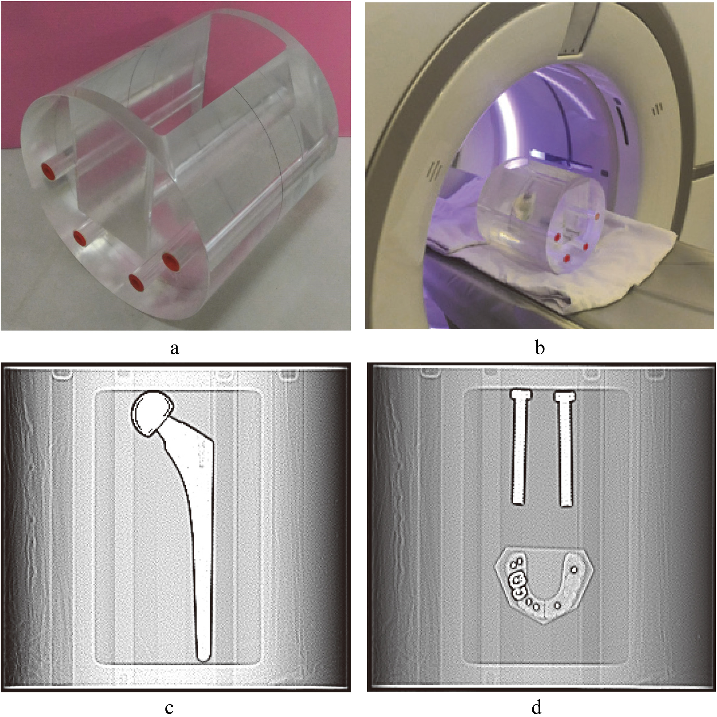
A cylindrical phantom was made from acrylic with a diameter of 20 cm and a length of 24 cm. A rectangular groove with a length of 20 cm, the width of 10 cm, and a depth of 16 cm was on the side of the phantom (Fig. 1). Three types of metal implants were (1) a one-sided artificial hip joint (vitallium,
The groove of the phantom was filled with water after metal implants were placed into it. Therefore, the metal implants were surrounded by water, which could be used for analyzing the degree to which metal artifact affected the CT number of the water (Fig. 1).
Figure 1.
Customized acrylic phantom and scanned images. a. A cylindrical phantom with a rectangular groove in the side of the phantom. b. The phantom with metal implant is placed on the platform of a CT scanner. c. Scout image of hip implant. d. Scout image of spinal implant and dental filling.
2.2Image acquisition
The cylindrical phantom containing metal implants was scanned by CT of four manufacturers (Fig. 1): Canon Aquilion One Vision Edition (Canon Medical Systems, Otawara, Japan); GE Revolution CT (GE Healthcare, Milwaukee, WI, USA); Siemens Somatom Definition AS (Siemens Healthcare, Erlangen, Germany); Philips iCT 256 (Philips Healthcare, Best, Netherlands). The scanning protocols of each scanner are shown in Table 1. The parameters of all CT scans are frequently used in clinical settings.
Table 1
CT scan parameter
| Parameter | CT scan parameters | |||
|---|---|---|---|---|
| Canon Medical Systems (Otawara, Japan) | GE Healthcare (Milwaukee, WI) | Siemens Healthcare (Erlangen, Germany) | Philips Healthcare (Best, Netherlands) | |
| Scanner type | Canon Aquilion ONE ViSION Edition (SE) | Revolution CT (DE by fast kV switching) | Siemens SOMATOM | Philips iCT 256 (SE) |
| CT protocol | Volume (SEMAR not compatible with helical scanning) | Helical (pitch 1) | Helical (pitch 1) | Helical (pitch 1) |
| Rotation time | 0.5 | 0.5 | 0.5 | 0.5 |
| Tube voltage (kVp) | 120 | DE: 80/140 | DE: 100/140 | 120 |
| CTDI | 9.2 | 10.1 | 10.3 | 10.4 |
| Collimation (mm) | 160 | 128 | 128 | 128 |
| Slice thickness (mm) | 0.5 | 0.625 | 0.6 | 0.8 |
| Reconstruction FOV (mm) | 300 | 300 | 300 | 300 |
| MAR technique | SEMAR | Smart-MAR | IMAR | OMAR |
| IR technique | AIDR 3D Level standard 50% | ASIR Level 50% | SAFIRE Level 3 | IDOSE Level 3 |
| Kernel | FC08 | Standard | Q30 | Standard B |
SE, single energy; DE, dual energy; CTDIvol, volume CT dose index; MAR, metal artifact reduction; IR, iterative reconstruction.
0.5 seconds was chosen for the rotation time of the gantry. The pitch was set at 1.0 to prevent overlapping scans and the distortion of CT images caused by interpolation of the data. The volume CT dose index (CTDI
After obtaining images from four CT scanners, MAR technique of each scanner was applied to images. The Canon CT scanner of this study was operated with single energy of 120 kVp and in axial scan mode only because the SEMAR technique cannot be used in the helical scan mode. The dual energy mode (80/140 kV) and 120 keV monoenergetic images were chosen when using the GE CT. The helical mode was chosen for GE scanner because the Smart-MAR technique in axial mode has a limited scan range (40 mm). IMAR can be used both in single and dual energy modes when using the Siemens CT, but only dual energy images were presented because the quality of dual energy images was considerably higher than the quality of single energy images. The dual energy technique used 140/100 kV and energy modules of 120 keV for Siemens scanner. When using IMAR, different types of IMAR mode could be selected according to the type of metal implant. Hip implants, dental mode, and spinal implant mode of IMAR were applied to images of Siemens scanner in this work. The Philips iCT scanner in this study only provides a single energy mode, and the thickness of its smallest slice was 0.8 mm with a pitch of 1; the slice was slightly thicker than those of the other CT scanners. OMAR of Philips can be applied to images before or after the scan.
2.3Quantitative assessment
2.3.1Metal volume
ImageJ (Java 1.8, National Institutes of Health, Bethesda, USA) software was used to measure the area of metal implants (
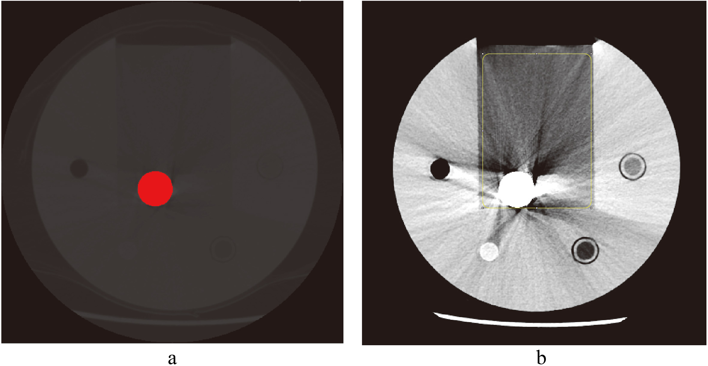
Figure 2.
Measurement of metal volume and fraction of bad pixel area (FBPA). a. Volume of hip implant in red region. b. Measurement of fraction of bad pixel area (FBPA) of hip implant in a rectangular area of 10000 mm
The volume of a metal object
(1)
The slice thickness of each scanner is listed in Table 1. The length of hip implant and titanium rods are 195 and 75 mm respectively, and the total numbers of slices of each group of CT images will be different due to different slice thicknesses. The volume of dental fillings was not measured because the metal was close to denture which CT number was also relatively high, and it is difficult to distinguish the metal, denture, and artifact from each other with a fixed threshold.
We subtracted the volume of metal implants
(2)
2.3.2Fraction of bad pixel area (FBPA)
In the study by Bolstad et al. [24], a threshold above 500 HU was chosen for evaluating the degree of artifacts. However, metal artifacts also consist of dark bands or low-intensity zone, and a high-level threshold could not evaluate the dark zone. In this study, we circled a rectangular zone with an area of 10,000 mm
(3)
The rectangular zone contained only water and metal objects, and thus CT numbers other than these two materials were noises and CT number errors caused by metal artifacts. The FBPA might also change according to a different threshold of water, but the differences remain between four CT scanners if the same threshold was chosen for measuring all images.
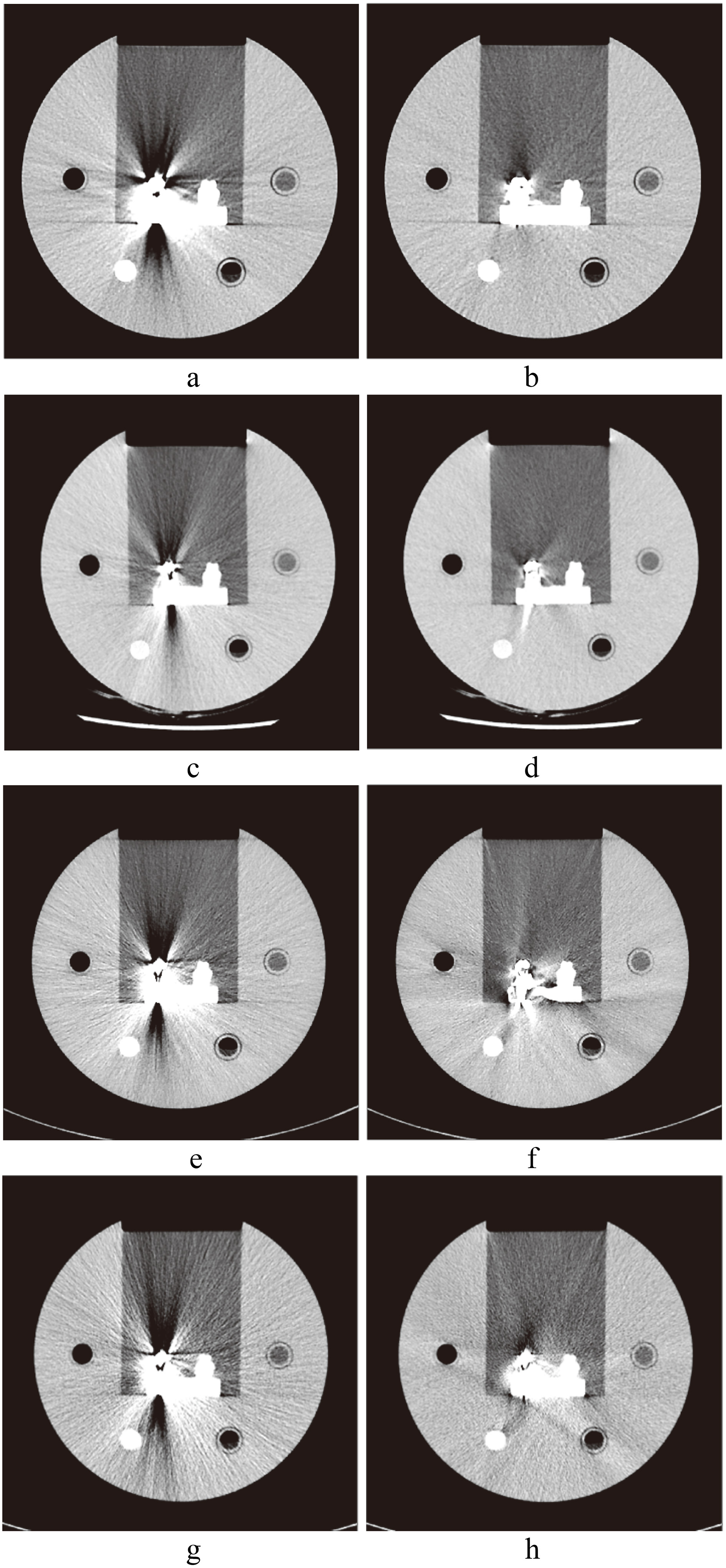
Figure 3.
CT images of hip implants. a. Image without SEMAR; b. with SEMAR. c. Image without Smart-MAR; d. with Smart-MAR. e. Image without IMAR; f. with IMAR. g. Image without OMAR; h. with OMAR.
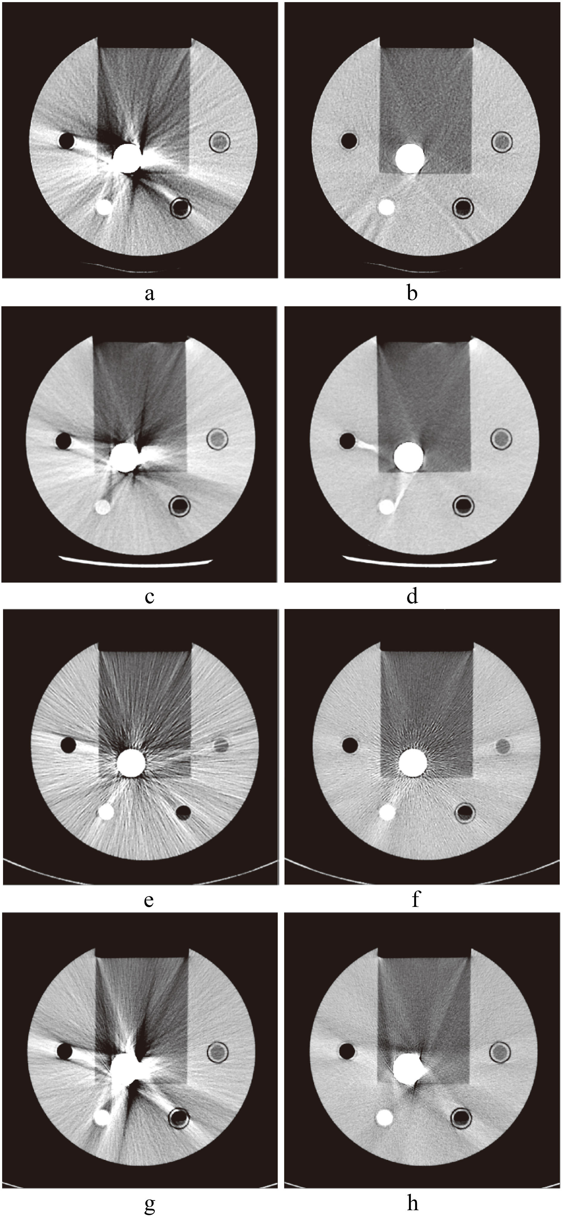
Figure 4.
CT images of spinal implants. a. Image without SEMAR; b. with SEMAR. c. Image without Smart-MAR; d. with Smart-MAR. e. Image without IMAR; f. with IMAR. g. Image without OMAR; h. with OMAR.
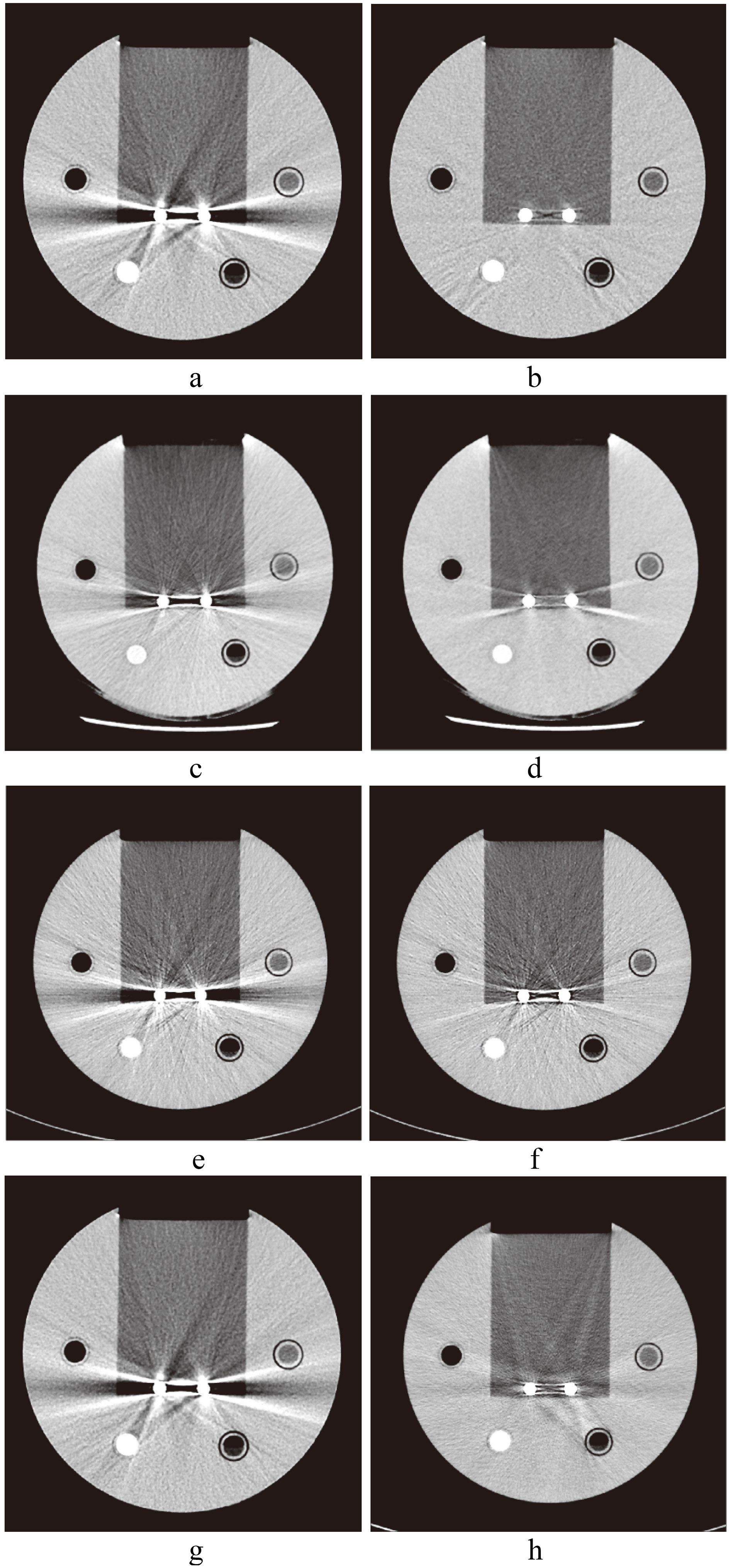
Figure 5.
CT images of dental filling. a. Image without SEMAR; b. with SEMAR. c. Image without Smart-MAR; d. with Smart-MAR. e. Image without IMAR; f. with IMAR. g. Image without OMAR; h. with OMAR.
We calculated the FBPA of all CT images of each type of metal implant and obtained the average FBPA. The FBPA of hip implant was divided into two parts (head and body) because the difference in the metal area of image cross-sections of the hip implant is too large; the spinal implant was in a cylindrical shape, and calculating the average of FBPA for all metallic images directly would suffice. Differences in the metal area of each cross-section of dental filling were overly large; the average value of FBPA of it was calculated directly. The FBPA improvement value was calculated by subtracting the average FBPA value of uncorrected images (
(4)
2.3.3Visual ranking analysis
The image containing the most severe artifacts was selected for evaluation. A total number of 24 images were chosen (Figs 3–5); three metal implants, four scanners, and two images per scanner (with and without MAR). Eight images (with and without MAR from four vendors of each metal implant) were anonymized and randomized compared as one group for three times by each reviewer. Two radiologists (15 and 18 years of experience) and one radiographer (17 years of experience) were invited to review the image quality. The reviewers evaluated the CT images and ranked the images that optimally visualized the water area surrounding metal implants from the best to worst (first to eighth). After the ranking has been done, the best to the fourth images were scored 4, 3, 2, and 1, respectively, and the rest were scored 0.
2.3.4Statistical method and figure of merit (FOM)
One-way analysis of variance and the Bonferroni post hoc test were used to examine the differences of FBPA improvements between four MAR techniques. Kendall coefficient of concordance was used to evaluate the consistency between observers of visual ranking analysis.
The total quantitative results that combined subjective and objective evaluation for each MAR technique were defined by the figure of merit. The average and standard deviation of visual ranking scores for each metal implant were used for the calculation of the expected value (
(5)
The key kernel of FOM is trying to quantify the digitized performance from various factors in the study. The definition of FOM herein is defined to fulfill “larger-the-better” tendency, therefore a high FBPA improvement or visual ranking score is always preferable whereas a low FBPA or standard deviation is preferable. Furthermore, the FOM tries to integrate all the performances of various CT scanners in one rule of thumb, thus, all the implanted materials have to be considered thoroughly to obtain a compiled digitized index for comparison among CT scanners.
Table 2
Metal implant volume results
| Image sequence | Hip implant volume (mm | Spinal implant volume (mm |
|---|---|---|
| Canon | ||
| Original | 59274.8 | 13845.5 |
| SEMAR | 54898.2 | 13340.2 |
| Improvement (%) | 7.4 | 3.6 |
| GE | ||
| Original | 55596.1 | 13561.9 |
| Smart-MAR | 55139.9 | 13699.7 |
| Improvement (%) | 0.8 | |
| Siemens | ||
| Original | 57813.8 | 14150.9 |
| IMAR | 57304.1 | 13904.4 |
| Improvement (%) | 0.9 | 1.7 |
| Philips | ||
| Original | 59798.3 | 15197.7 |
| OMAR | 57630.4 | 14322.6 |
| Improvement (%) | 3.6 | 5.8 |
3.Results
3.1Objective analysis
The results of metal volume measurement are shown in Table 2. In the original images, the hip implant and spinal implant in GE’s images measured the smallest volumes (55,596.1 mm
With hip implants, the optimal metal volume improvement rate was Canon’s 7.4%, followed by 3.6% for Philips. No obvious improvement was found in the images of GE and Siemens, which achieved rates of 0.8% and 0.9%. With spinal implants, the optimal metal volume improvement rate was 5.8% for Philips, followed by 3.6% of Canon. It is noteworthy that the metal volume of GE showed no improvement (less than 0%).
Table 3
Results of FBPA improvement, visual ranking score, and expected value
| MAR | SEMAR | Smart-MAR | p value | IMAR | p value | OMAR | p value | ||||
| FBPA improvement (%) | |||||||||||
| Hip implant (Head) | 33.7 | 32.3 | 0.320 | 20.0 | 18.2 | ||||||
| Hip implant (Body) | 7.0 | 0.8 | 2.4 | 5.4 | |||||||
| Spinal implant | 14.0 | 8.9 | 3.8 | 12.6 | |||||||
| Dental filling | 10.6 | 9.1 | 0.182 | 6.1 | 5.7 | ||||||
| Visual ranking score | |||||||||||
| Hip implant | 3.6 | 3.3 | – | 2.1 | – | 0.9 | |||||
| Spinal implant | 3.9 | 3.1 | – | 1.4 | – | 0.9 | 0.001 | ||||
| Dental filling | 3.1 | 3.8 | – | 1.3 | – | 0.3 | 0.002 | ||||
| Expected value | 36.6 | 37.8 | 5.0 | 2.3 | |||||||
For FBPA improvement, all
Figure 6.
Measurement results of fraction of bad pixel area (FBPA) of three metal implants. Hip implant is divided into two parts; head and body.
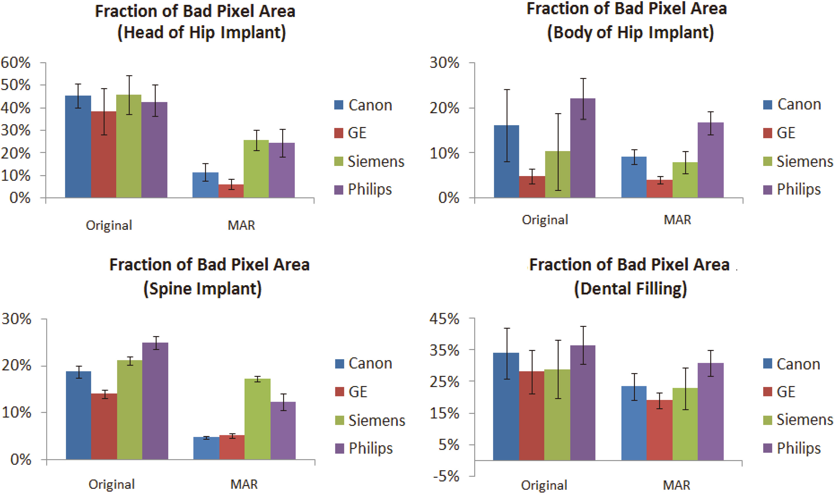
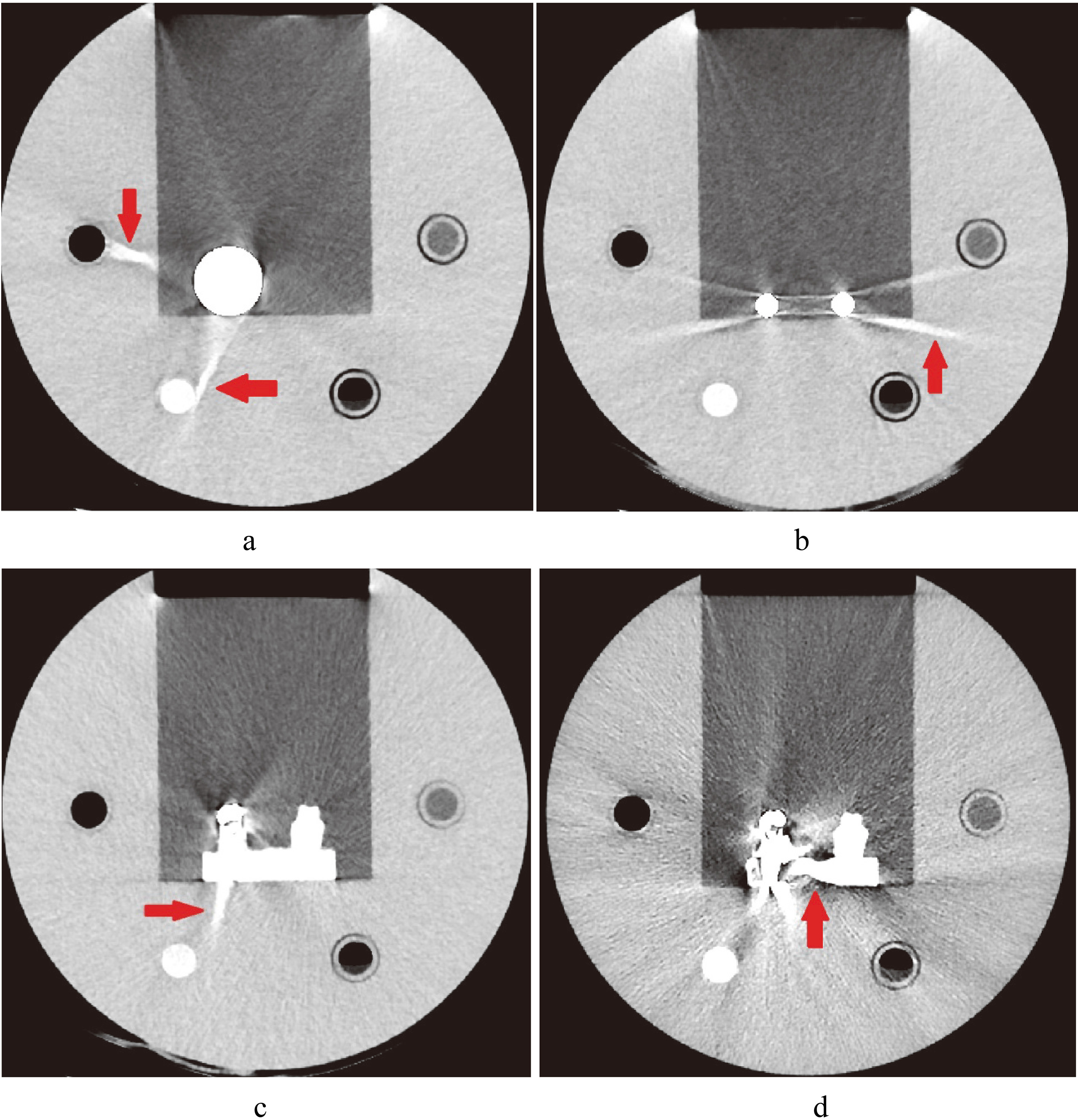
Figure 7.
Images of artifacts caused by MAR. a. Image of hip implant with artifact caused by Smart-MAR (red arrow). b. Image of spinal implant with artifact caused by Smart-MAR (red arrow). c. Image of dental filling with artifact caused by Smart-MAR (red arrow). d. Image of dental filling with artifact caused by IMAR (red arrow).
The results of FBPA are shown in Fig. 6. The FBPA of reference images without metal implants (with and without MAR) both are 0.1%. The FBPA of the head of hip implants found using an MAR technique with Canon, GE, Siemens, and Philips machines were 11.6
FBPA improvement rate results of groups of images after using a MAR technique are shown in Table 3. In the head of hip implant images, the optimal improvement rate was 33.7
3.2Subjective analysis and FOM
The results of average ranking scores by the three experienced experts are shown in Table 3. The SEMAR technique of Canon was optimal for hip and spinal implants; and the Smart-MAR technique of GE for dental filling. The OMAR technique of Toshiba achieved the least desirable results in all types of metal implants.
The expected values of four MAR techniques are also shown in Table 3. The greatest value was 37.8 of Smart-MAR and second value was 36.6 of SEMAR. The performance of IMAR and OMAR were only 5.0 and 2.3.
4.Discussion
4.1Quantitative comparison
Of the four MAR techniques, Smart-MAR and SEMAR are superior to the other two, which is in line with the results of Bolstad et al. [24]. The SEMAR technique has better FBPA improvement for all the metal implants and better visual ranking scores for hip and spinal implants then Smart-MAR, but still Smart-MAR reaches the greatest expected value. The reason for this is Smart-MAR has the smallest FBPA value in all images except for the images of spinal implants. The metal volume and FBPA of GE’s original image attained the optimal performance mainly because of the overall performance of its CT scanner (dual energy and lesser noise). The improvement rate of metal volume was not included in the figure of merit because of the lack of metal volume of dental filling.
The images of metal implants after correction of the Smart-MAR produced new artifacts in the acrylic part of the phantom (Fig. 7). This showed that the Smart-MAR may exhibit errors for materials with a CT number higher than water when reducing streak artifacts produced by the metal. The images of dental filling after using IMAR also produced new artifacts (Fig. 7). With the spinal implant, an obvious artifact remained in the central zone of the two titanium rods for all four types of MAR techniques (Fig. 4).
The performance of the four MAR techniques in improving artifacts produced by the dental filling was less satisfactory than the other two metal implants (Fig. 5). This was because the density of the amalgam alloy in the dental filling (
On the basis of the results from analyzing the three aforementioned metal implants, this study suggests that the FBPA improvement and objective visual ranking were nearly the same. The measurement and improvement of FBPA are similar to the study of Huang et al. [25]. Huang et al. calculated the HU error (bad pixel) map by subtracting the baseline image from the metal image (excluding regions of air and the metal implant). FBPA only calculated bad pixel area within the same image, which is easier to perform and has less experimental errors. This is an effective and objective quantitative method for evaluating the optimal adjustment for various MAR techniques.
4.2Comparison with previous studies
Bolstad et al. compared surgical sheet metal made of three types of materials on leg phantoms using subjective and objective quantitative analysis of four MAR techniques [24]. The results of the subjective quantitative analysis showed that SEMAR had superior performance in two types of metal with lower densities compared with the other three MAR techniques. Smart-MAR achieved the optimal performance in metal with relatively high density, which is highly consistent with the spine implant analysis results in this study. The objective analysis of Bolstad et al. focused on the CT number of fractions of pixels higher than 500 HU in the area surrounding metal implants; the metal volume they found was consistent with that of this study. However, their objective measurement was unable to analyze the effect of metal artifacts on the surrounding soft tissue. The FBPA proposed in this study can evaluate the degree to which a metal artifact influences the water and adjacent soft tissue CT number.
Wagenaar et al. used an objective method to analyze the effect of three techniques (Smart-MAR, OMAR, and IMAR) on a head phantom with a dental filling [23]. The errors of CT number of Smart-MAR and OMAR were extremely close and were higher than IMAR, but the study did not analyze SEMAR. In the dental filling analysis of this study, SEMAR attained the optimal results of subjective and objective analyses, followed by Smart-MAR, OMAR (third place), and IMAR. Our study results are highly similar to those of Wagenaar et al., but we added an analysis of SEMAR.
Anderson et al. used subjective and objective quantitative methods to analyze the effect of OMAR and SEMAR in hip implants [20, 21]. When the soft kernel was forming images, VGA ratings of the two techniques were the same, which is inconsistent with our finding that SEMAR was superior to OMAR. However, the study by Anderson et al. used an artificial phantom with a double-sided hip implant, which is different from the single hip implant in this study. Another difference is that this study simultaneously analyzed the hip implant using four MAR techniques (SEMAR, Smart-MAR, IMAR, and OMAR).
4.3Limitations
This work evaluated four commercial MAR techniques on three common types of metal implants in a clinical setting for the first time. However, there are limitations to the study. Dual-energy technique has been available with MAR for Philips scanners in a recent update, and CT images with dual-energy cause lesser noise [8]. The helical mode with the MAR for Canon scanner has also been made available recently and can provide more insight into comparison.
The scan protocols used in the study were all common conditions used in clinical settings and were not optimally adjusted with the MAR technique for each scanner. Therefore, the performance was not optimal for four vendors. The best MAR conditions for each vendor should be studied in future work.
5.Conclusion
This study successfully used subjective and objective quantitative methods to evaluate the effect of using four commercial MAR techniques on three types of metal implants (hip implant, spinal implant, and dental filling) in a phantom for the first time in literature. All four MAR techniques effectively reduced metal artifacts, but the effect deteriorated when applied to dental fillings with higher amalgam alloy density. SEMAR of Canon and Smart-MAR of GE achieved optimal subjective and objective analysis results for the three types of metal implants among four MAR techniques.
Conflict of interest
None to report.
References
[1] | Man BD, Nuyts J, Dupont P, Marchal G, Suetens P. Metal streak artifacts in X-ray computed tomography: A simulation study. IEEE Transactions on Nuclear Science (1999) ; 46: : 691–6. doi: 10.1109/23.775600. |
[2] | Robertson DD, Weiss PJ, Fishman EK, Magid D, Walker PS. Evaluation of CT techniques for reducing artifacts in the presence of metallic orthopedic implants. Journal of Computer Assisted Tomography (1988) ; 12: : 236–41. doi: 10.1097/00004728-198803000-00012. |
[3] | Omar G, Abdelsalam Z, Hamed W. Quantitative analysis of metallic artifacts caused by dental metallic restorations: Comparison between four CBCT scanners. Future Dental Journal (2016) ; 2: : 15–21. doi: 10.1016/j.fdj.2016.04.001. |
[4] | Enomoto Y, Yamauchi K, Asano T, Otani K, Iwama T. Effect of metal artifact reduction software on image quality of C-arm cone-beam computed tomography during intracranial aneurysm treatment. Interventional Neuroradiology (2018) ; 24: : 303–8. doi: 10.1177/1591019917754039. |
[5] | Gjesteby L, Man BD, Jin Y, Paganetti H, Verburg J, Giantsoudi D, et al. Metal artifact reduction in CT: Where are we after four decades? IEEE Access (2016) ; 4: : 5826–49. doi: 10.1109/access.2016.2608621. |
[6] | Pan Y-N, Chen G, Li A-J, Chen Z-Q, Gao X, Huang Y, et al. Reduction of metallic artifacts of the post-treatment intracranial aneurysms: Effects of single energy metal artifact reduction algorithm. Clinical Neuroradiology (2017) . doi: 10.1007/s00062-017-0644-2. |
[7] | Asano Y, Tada A, Shinya T, Masaoka Y, Iguchi T, Sato S, et al. Utility of second-generation single-energy metal artifact reduction in helical lung computed tomography for patients with pulmonary arteriovenous malformation after coil embolization. Japanese Journal of Radiology (2018) ; 36: : 285–94. doi: 10.1007/s11604-018-0723-6. |
[8] | Ohira S, Kanayama N, Wada K, Karino T, Nitta Y, Ueda Y, et al. How well does dual-energy computed tomography with metal artifact reduction software improve image quality and quantify computed tomography number and iodine concentration? Journal of Computer Assisted Tomography (2018) ; 1. doi: 10.1097/rct.0000000000000735. |
[9] | Zhou P, Zhang C, Gao Z, Cai W, Yan D, Wei Z. Evaluation of the quality of CT images acquired with smart metal artifact reduction software. Open Life Sciences (2018) ; 13: : 155–62. doi: 10.1515/biol-2018-0021. |
[10] | Huang VW, Kohli K. Evaluation of new commercially available metal artifact reduction (MAR) algorithm on both image quality and relative dosimetry for patients with hip prosthesis or dental fillings. International Journal of Medical Physics, Clinical Engineering and Radiation Oncology (2017) ; 6: : 124–38. doi: 10.4236/ijmpcero.2017.62012. |
[11] | Wei J, Schabel C, Bongers M, Raupach R, Clasen S, Notohamiprodjo M, et al. Impact of iterative metal artifact reduction on diagnostic image quality in patients with dental hardware. Acta Radiologica (2016) ; 58: : 279–85. doi: 10.1177/0284185116646144. |
[12] | Long Z, Bruesewitz MR, Delone DR, Morris JM, Amrami KK, Adkins MC, et al. Evaluation of projection- and dual-energy-based methods for metal artifact reduction in CT using a phantom study. Journal of Applied Clinical Medical Physics (2018) ; 19: : 252–60. doi: 10.1002/acm2.12347. |
[13] | Diehn FE, Michalak GJ, Delone DR, Kotsenas AL, Lindell EP, Campeau NG, et al. CT dental artifact: Comparison of an iterative metal artifact reduction technique with weighted filtered back-projection. Acta Radiologica Open (2017) ; 6: : 11. doi: 10.1177/2058460117743279. |
[14] | Ali A. Evaluation of orthopedic metal artifact reduction application in three-dimensional computed tomography reconstruction of spinal instrumentation: A single saudi center experience. Journal of Clinical Imaging Science (2018) ; 8: : 11. doi: 10.4103/jcis.jcis_92_17. |
[15] | Rim J, Choi J-A, Lee SA, Khil EK. Comparison of metal artifact reduction for orthopedic implants versus standard filtered back projection: Value of postoperative CT after hip replacement. Journal of the Korean Society of Radiology (2018) ; 78: : 22. doi: 10.3348/jksr.2018.78.1.22. |
[16] | Giantsoudi D, Man BD, Verburg J, Trofimov A, Jin Y, Wang G, et al. Metal artifacts in computed tomography for radiation therapy planning: Dosimetric effects and impact of metal artifact reduction. Physics in Medicine and Biology (2017) ; 62. doi: 10.1088/1361-6560/aa5293. |
[17] | Long Z, Bruesewitz MR, Delone DR, Morris JM, Amrami KK, Adkins MC, et al. Evaluation of projection- and dual-energy-based methods for metal artifact reduction in CT using a phantom study. Journal of Applied Clinical Medical Physics (2018) ; 19: : 252–60. doi: 10.1002/acm2.12347. |
[18] | ang J, Zhang D, Wilcox C, Heidinger B, Raptopoulos V, Brook A, et al. Metal implants on CT: Comparison of iterative reconstruction algorithms for reduction of metal artifacts with single energy and spectral CT scanning in a phantom model. Abdominal Radiology (2017) ; 42: : 742–8. doi: 10.1007/s00261-016-1023-1. |
[19] | Kidoh M, Utsunomiya D, Oda S, Nakaura T, Funama Y, Yuki H, et al. CT venography after knee replacement surgery: Comparison of dual-energy CT-based monochromatic imaging and single-energy metal artifact reduction techniques on a 320-row CT scanner. Acta Radiologica Open (2017) ; 6: : 2. doi: 10.1177/2058460117693463. |
[20] | Andersson KM, Norrman E, Geijer H, Krauss W, Cao Y, Jendeberg J, et al. Visual grading evaluation of commercially available metal artefact reduction techniques in hip prosthesis computed tomography. The British Journal of Radiology (2016) ; 89: : 1063. doi: 10.1259/bjr.20150993. |
[21] | Andersson KM, Nowik P, Persliden J, Thunberg P, Norrman E. Metal artefact reduction in CT imaging of hip prostheses – an evaluation of commercial techniques provided by four vendors. The British Journal of Radiology (2015) ; 88: : 1052. doi: 10.1259/bjr.20140473. |
[22] | Andersson KM, Dahlgren CV, Reizenstein J, Cao Y, Ahnesjö A, Thunberg P. Evaluation of two commercial CT metal artifact reduction algorithms for use in proton radiotherapy treatment planning in the head and neck area. Medical Physics (2018) ; 45: : 4329–44. doi: 10.1002/mp.13115. |
[23] | Wagenaar D, Graaf ERVD, Schaaf AVD, Greuter MJW. Quantitative comparison of commercial and non-commercial metal artifact reduction techniques in computed tomography. Plos One (2015) ; 10. doi: 10.1371/journal.pone.0127932. |
[24] | Bolstad K, Flatabø S, Aadnevik D, Dalehaug I, Vetti N. Metal artifact reduction in CT, a phantom study: Subjective and objective evaluation of four commercial metal artifact reduction algorithms when used on three different orthopedic metal implants. Acta Radiologica (2018) ; 59: : 1110–8. doi: 10.1177/0284185117751278. |
[25] | Huang J, Kerns J, Nute J, Liu X, Balter P, Stingo F, Followill D, Mirkovic D, Howell R, Kry S. An evaluation of three commercially available metal artifact reduction methods for CT imaging. Physics in Medicine and Biology (2015) ; 60: (3): 1047–67. doi: 10.1088/0031-9155/60/3/1047. |
[26] | Yeh D, Wang T, Pan L. Evaluating the quality characteristics of TLD-100T and TLD-100H exposed to diagnostic X-rays and 64 multislice CT using Taguchi’s quality loss function. Radiation Measurement (2015) ; 80: : 17–22. |

