
BGRF: A broad granular random forest algorithm
Abstract
The random forest is a combined classification method belonging to ensemble learning. The random forest is also an important machine learning algorithm. The random forest is universally applicable to most data sets. However, the random forest is difficult to deal with uncertain data, resulting in poor classification results. To overcome these shortcomings, a broad granular random forest algorithm is proposed by studying the theory of granular computing and the idea of breadth. First, we granulate the breadth of the relationship between the features of the data sets samples and then form a broad granular vector. In addition, the operation rules of the granular vector are defined, and the granular decision tree model is proposed. Finally, the multiple granular decision tree voting method is adopted to obtain the result of the granular random forest. Some experiments are carried out on several UCI data sets, and the results show that the classification performance of the broad granular random forest algorithm is better than that of the traditional random forest algorithm.
1Introduction
Ensemble learning is a machine learning algorithm, which is widely used in intrusion detection [1], network security [2], emotion recognition [3], image denoising [4], and so on. The ensemble classifier establishes multiple training models on the data set and constructs multiple independent or related base classifiers. The ensemble classifier will integrate the results of various base classifiers to improve the model’s classification performance and running time [5].
The random forest is an ensemble learning algorithm proposed by Breiman in 2001 [6]. The algorithm uses the bagging [7] ensemble to combine multiple decision trees into a forest. At the same time, the random subspace theory is introduced into the training data set and the characteristics of the data set. So random forest solves the overfitting problem of decision trees. In recent years, many scholars have improved the random forest to enhance the performance of the algorithm. Yates [8] et al. improved the processing speed of random forests while maintaining accuracy. Sun [9] et al. proved the consistency of the algorithm by combining the random forest and the Shapley value. Han [10] et al. proposed the double random forest to further improve the prediction accuracy. Random forest is suitable for large data sets, which makes it develop rapidly. Random forest algorithm has been widely used in many fields, such as image classification [11], speech emotion recognition [12], fault diagnosis [13], face recognition [14], and risk assessment [15].
The number of decision trees will greatly affect the classification effect of random forests. If the number of decision trees is too small, the fitting ability is not enough, which will reduce the accuracy of classification. However, if the number of decision trees is too large, the generalization ability is not enough, which leads to the reduction of the classification effect. In 2021, Pavlov [16] studied the maximum number of decision trees in a random forest. How to choose the appropriate number of decision trees is also a hot topic in random forest research.
The random forest improves the classification effect of the decision tree algorithm in large data sets. However, the random forest algorithm has poor classification accuracy in the face of data sets with small dimensions. To solve this problem, a granular classifier is established on granular computing theory. Granular computing is a new concept and method in the field of artificial intelligence. Granular computing is mainly used to deal with uncertain information and solve complex problems. Granular computing transforms complex problems into several simple problems and abstracts information granules from information or data according to a certain characteristic. In 1997, Zadeh [17] first proposed a general framework for the study of fuzzy information granule theory. In response to Zadeh’s point of view, many researchers have joined the research work of information granules. In 2013, Yao [18] et al. discussed and sorted out the application fields and research directions of granular computing theory. The main models of granular computing are fuzzy sets [19, 20], rough sets [21, 22], concept-cognitive learning [23, 24], three-way decision [25, 26], and so on. With the rapid development in recent years, granular computing has been successfully applied in many fields. Zhang [27] et al. combined granular computing with multi-label active learning to improve the accuracy of the algorithm. Fu [28] et al. proposed a granular computing framework for hierarchical community detection. Wei [29] et al. used information granulation to improve the ReliefF algorithm. Wang [30] et al. modeled the multi-granularity decision problem from the perspective of uncertainty.
Data granulation is the basis of data analysis based on granular computing theory. Data granulation is the process of breaking down complex data into smaller data granules. The methods of data granulation include fuzzy granulation [31], knowledge granulation [32], neighborhood granulation [33, 34], and so on. In 2018, Chen [35] et al. proposed a broad learning system and designed a planar network. Because the traditional classifier is not easy to deal with uncertain data. To improve the performance of the traditional classifier, a broad granulation method is proposed based on the broad structure. The structure of granules is designed to be flat, which reduces the complexity of the granule’s operation. The granules are essentially a set, so granular computing is a set of operations. Data granulation is a common technology and method in granular computing, but there are a few examples of the combination of granulation and a classifier. This paper proposes a new granular random forest algorithm based on broad granulation. The samples form the broad granules through the granulation of the relationship between the features, and the broad granules constitute a broad granular vector. The new features of broad granules and granular vectors are defined, and then the granular decision tree model is constructed. The bagging and random strategies are further designed, and a granular random forest algorithm is proposed. From the perspective of binary classification and multi-classification, the effect of the size of the granular random forest on the performance of the algorithm is discussed. By designing the broad granular random forest algorithm, the classification of the data is successfully realized. Finally, the experimental analysis verifies the correctness and effectiveness of the broad granular random forest algorithm.
The rest of the paper is organized as follows. Section 2 introduces the particle and particle vectors. Then we propose the broad granulation, and how the granules operate. In Section 3, the granular random forest algorithm is introduced, and then we propose a granular decision tree, which serves as the base classifier of a granular random forest. In addition, we combine the proposed broad granulation technique with the idea of random forest classification to propose the broad granulation random forest algorithm, which helps to improve the classification effect in binary and multi-classification problems. In Section 4, some experiments are conducted to show the effectiveness of our proposed method. Finally, the results of the study and future work are discussed in Section 5.
2Broad granulation
A granule is an orderly collection, while a granular vector is made up of granules. The operators related to granular vectors are easy to be restricted and are not easy to be extended and applied. The broad learning system is to transform the deep network of deep learning into a plane network. In this paper, we design flat granules to form a flat granular vector through the relationship between the data features. Broad granulation changes the dimensionality of the original data and forms new features. Furthermore, the granular features related to the broad granules and granular vectors are defined, and the granular classifier is constructed.
2.1Granules and granular vectors
Definition 1. Let the set ga ={ z1, z2, . . . , zn }, where zi ∈ Z, then the set is defined as the granule, and the set cardinality of the granule is its dimension, then the n-dimensional granule is represented as
(1)
Definition 2. Let
(2)
The granular vector is composed of granules, and the granules are an orderly set. Thus, the elements of a granular vector are also orderly sets.
2.2Broad granulation and broad granules
The elements in the granular vectors are arranged in order. To better handle granular vectors, we use lateral thinking to granulate. A feature is selected from the data set, and then multiple features are extracted from the data set as the reference features for granulation. The sample is broadly granulated in the reference features to form broad granules. All data are broadly granulated, and the broad granules of the same sample are combined into broad granular vectors.
Let the information learning system be U = (X, C ∪ B, f), where the data set is X ={ x1, x2, . . . , xm } and the characteristic set is C ={ c1, c2, . . . , cn }. The reference feature set is B ={ b1, b2, . . . , bk }, B ⊑ C, and k ≤ n. The f is an information function.
Definition 3. Let the information learning system be U = (X, C ∪ B, f), where the reference is a feature subset B ⊑ C. The granule is ga ={ z1, z2, . . . , zn }, and n = k. Then the broad feature set of the granule can be expressed as
(3)
Definition 4.Let the information learning system be U = (X, C ∪ B, f). For the training sample x ∈ X. A single feature c ∈ C and a broad feature b ∈ B, then the breadth of x over c and b is
(4)
Definition 5. Let the information learning system be U = (X, C ∪ B, f), a single sample x ∈ X, a single feature c ∈ C and a broad feature set B ={ b1, b2, . . . , bk }, then the breadth of x in the feature c and the broad feature is granulated, and the broad granule formed is defined as
(5)
Definition 6. Let the information learning system be U = (X, C ∪ B, f), a single sample x ∈ X, the broad granule g ={ z1, z2, . . . , zk } of x, and C ={ c1, c2, . . . , cn }, then the broad granular vector of x is defined as
(6)
(7)
(8)
Definition 7. Let the information learning system be U = (X, C ∪ B, f), where the broad feature set B ⊑ C and the broad granular vector is G (x) = {[z11, z12, . . . , z1k] , [z21, z22, . . . , z2k] , . . . , [zn1, zn2, . . . , znk]}, then the granular features set of the information learning system can be expressed as
(9)
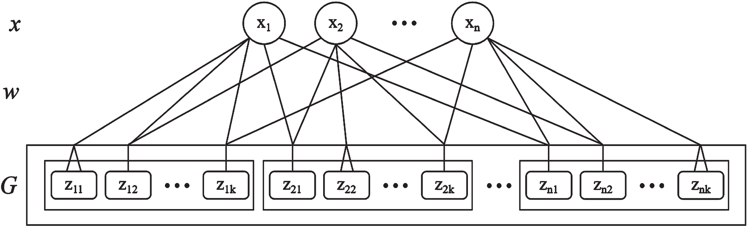
Broad granulation is the process of building broad granules and broad granular vectors. The process of broad granulation is shown in Fig. 1. For a data set X, each sample has a feature set C ={ c1, c2, . . . , cn }. For convenience, the feature set C is labeled with an integer, then the sample vector is x ={ x1, x2, . . . , xn }. The sample is broadly granulated between features through w, where w is the broad formula of Definition 4. Then, the constructed broad granules g ={ z1, z2, . . . , zk } are merged into a broad granular vector G. The broad feature set is B ={ b1, b2, . . . , bk }, and a new feature is formed after the sample feature and the feature of the granules are recombined and adjusted. The last broad granular vector is G (x) = {[z11, z12, . . . , z1k] , [z21, z22, . . . , z2k] , . . . , [zn1, zn2, . . . , znk]}.
Fig. 1
A process of broad granulation.
The advantage of broad granulation is that it is simple and easy to construct granular vectors. The broad granular vectors are input to a granular classifier to improve the performance of the granular classifier and obtain better results.
Example 1. Let the information learning system be U = (X, C ∪ B, f), as shown in Table 1. Suppose B = C, the broad granulation is as follows.
Table 1
An information learning system
| U | a | b | c |
| x1 | 0.2 | 0.7 | 0.5 |
| x2 | 0.1 | 0.2 | 0.4 |
| x3 | 0.5 | 0.6 | 0.1 |
The broad granules after the broad granulation of the sample x1 are g1 (x1) ={ 1, 0.5, 0.7 }, g2 (x1) ={ 0.5, 1, 0.8 }, g3 (x1) ={ 0.7, 0.8, 1 }, respectively.
The broad granules after the broad granulation of the sample x2 are g1 (x2) ={ 1, 0.9, 0.7 }, g2 (x2) ={ 0.9, 1, 0.8 }, g3 (x2) ={ 0.7, 0.8, 1 }, respectively.
The broad granules after the broad granulation of the sample x3 are g1 (x3) ={ 1, 0.9, 0.6 }, g2 (x3) ={ 0.9, 1, 0.5 }, g3 (x3) ={ 0.6, 0.5, 1 }, respectively.
The broad granular vector of the sample x1 is G (x1) ={ [1, 0.5, 0.7] , [0.5, 1, 0.8] , [0.7, 0.8, 1] }.
The broad granular vector of the sample x2 is G (x2) ={ [1, 0.9, 0.7] , [0.9, 1, 0.8] , [0.7, 0.8, 1] }.
The broad granular vector of the sample x3 is G (x3) ={ [1, 0.9, 0.6] , [0.9, 1, 0.5] , [0.6, 0.5, 1] }.
2.3Calculations of broad granules
The operations of the real numbers are closed on the real numbers, then the operations of the defined broad granules should also be closed on the broad granules.
Definition 8. Let
(10)
(11)
(12)
Definition 9. Let
(13)
(14)
(15)
Definition 10. Let G = [g1, g2, . . . , gB] be the broad granular vector, where
(16)
The broad granules need to be calculated in a granular classifier, so the calculation method of the broad granules is defined. Addition, subtraction, multiplication, and division of two broad granules result in one broad granule. After comparing the size of broad granules, the result is also broad granules. Broad granules can also calculate probabilities, and the probabilities of broad granules need to be added, subtracted, multiplied, and divided.
3The granular random forest algorithm
The granular classifier inputs the granular vector and granular feature and outputs a granular decision tree or the confidence of the category after granular computation. Therefore, the granular classifier can handle both binary and multi-class classification problems. The granular decision trees are parallelizable granular classifiers. The broad granules are a structured representation, and the components of the broad granules operate independently and are fully parallelizable. According to the characteristics of the broad granules, the granular random forest is designed. Broad granules can be separated and combined, which is the essence of a granular random forest.
3.1Granular decision trees
A granular decision tree is an algorithm that classifies granular vectors according to specified rules. A granular decision tree consists of granular nodes, leaf nodes, and directed edges. The broad granular node represents the granular features attribute of the granular vectors and can be divided into a root node and an intermediate node. The leaf node represents the class value of the granular vectors obtained by classifying the path of the granular vectors from the root node to the leaf node from top to bottom. A directed edge is a line connecting nodes from top to bottom. The goal of granular decision tree learning is to create a granular classifier through granular vector training. The granular classifier can effectively classify unknown granular vectors using a set of known granular vectors.
The granular decision tree learning method is mainly granular feature selection. The granular decision tree algorithm recursively selects the best features, resulting in the best classification process for each granule. In general, as the granular vectors continue to be split, it is required that the branching nodes of the granular decision tree contain as many granules from the same class as possible. That is, the node confusion degree of the granular decision tree becomes low. The granular Gini index is a key index to measure the disorder of granular vectors.
Definition 11.Let the information learning system be U = (X, C ∪ B, f), where the broad feature set is B ⊑ C, the broad granular vector is G (x) = [g (x) 1, g (x) 2, . . . , g (x) B]. The ratio of the granular vector of type c is pb (b = 1, 2, . . . , |yb|), then the granular Gini index of G is
(17)
(18)
The granular decision tree is used as the base classifier of a granular random forest to improve the classification performance of a granular random forest. The granular decision tree algorithm is described in Algorithm 1.
The condition for the algorithm to stop computing is that the granular Gini index is less than a predetermined threshold or that there are no more granular features.
Algorithm 1 Granular Decision Tree Algorithm (GDT)
Input: The information learning system is U = (X, C ∪ B, f);
Output:Granular decision tree.
1: X is normalized;
2: State The broad granulation of x on the broad features is gbi (x);
3: The broad granular vector forming x is GB (x) ={ gb1 (x) , gb2 (x) , . . . , gbi (x) };
4: Granular vector nodes are generated, and the granular Gini index of the existing granular feature pair G is calculated;
5: The granular feature with the smallest granular Gini index is selected as the cutting point to generate two granular nodes;
6: Repeat steps 4–5 for the granular nodes;
7: Generate a granular decision tree.
3.2The broad granular random forest algorithm
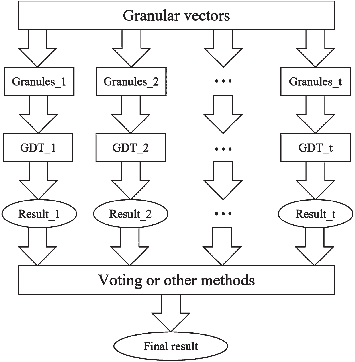
A granular random forest is an ensemble learning method based on a tree-shaped granular structure. Granular random forest is a powerful nonparametric granular computing method. Granular random forests can exert powerful performance in classification problems involving complex data sets. A granular random forest consists of many individual granular decision trees. These granular decision trees are grown by recursively performing binary segmentation on granular vectors. The granular random forest can reduce the variance of single granular decision tree classification and the deviation of classification results by averaging the classification results of a large number of granular decision trees. To ensure that there is a large enough variance in the granular decision tree to achieve this variance reduction, a granular randomness process is introduced into the tree growth process. Each granular decision tree is grown from different broad granules of the granular vectors. For each split, randomly selected granules are considered, not all granules. The principle of the granular random forest algorithm is shown in Fig. 2.
Fig. 2
The principle of a granular random forest algorithm.
Definition 12. Let the information learning system be U = (X, C ∪ B, f) and the broad granular vector be G (x) = [g (x) 1, g (x) 2, . . . , g (x) B], then the granules are voted, and the formula for determining the classification is as follows
(19)
Adjusting the parameters is an important part of using the granular random forest method, which can control the complexity of the random forest model. In a granular random forest, the number of granular decision trees needs to be set carefully. The advantage of particle random forest is that it can increase features and effectively ensure the classification accuracy of the model when there is a sample imbalance.
The granular feature selection method currently used is the granular Gini index. The granular decision tree in the granular random forest algorithm uses the granular Gini index probability model for granular feature selection. The principle of the particle Gini index is that the chaos degree of each particle node in the binary tree is the lowest. When all granular nodes belong to the same class, the granular Gini index value is the smallest. That is to say, the chaos degree of granular nodes is the lowest and the uncertainty of granular feature selection is small.
The combination of broad granulation and random forest can effectively improve the classification effect. A detailed description of the broad granular random forest algorithm is shown in Algorithm 2.
Algorithm 2 Broad Granular Random Forest Algorithm (BGRF)
Input: The information learning system is U = (X, C ∪ B, f), and the number of granular decision trees is T;
Output:The strong learner is f (x).
1: X is normalized;
2: The broad granulation of x on the broad features is gbi (x);
3: The broad granular vector forming x is GB (x) ={ gb1 (x) , gb2 (x) , . . . , gbi (x) };
4: Performing t times of random sampling with the replacement on the broad granular vectors, and acquiring n times in total to obtain a granule set Gt containing n-th granules;
5: Train the t-th granular decision tree model Gt (x) with the granular set Gt;
6: Train the granular nodes of GDT;
7: Select a portion of the features from all the granular features on the granular node of the binary tree;
8: Determine an optimal granular feature from the selected partial granular features by definition 11;
9: As the left and right subtrees of the granular decision tree, the optimal granular features are traversed and segmented continuously;
10: Set the number of iterations T;
11: Repeat steps 4–9 until the loop is stopped at the iteration number t = T;
12: The output is one or more categories with the maximum probability counted by T granular decision trees.
4Experimental analysis
The experiment uses 8 sets of standard data sets in the UCI database [36] for verification, and the specific information is shown in Table 2.
Table 2
The UCI data sets used in the experiment
| Data sets | Number of | Number of | Number of |
| sets | samples | features | categories |
| Ionosphere | 351 | 34 | 2 |
| Sonar | 208 | 60 | 2 |
| Heart | 270 | 13 | 2 |
| Bupa | 345 | 6 | 2 |
| Vowel | 990 | 13 | 11 |
| Newthyroid | 215 | 5 | 3 |
| Ecoli | 336 | 7 | 8 |
| Glass | 214 | 9 | 6 |
To test the classification effect of the granular random forest, each data set is randomly divided into two-thirds of the training set and one-third of the test set. According to the characteristics of the parameters of the granular random forest, this experiment sets the number of trees to verify the classification effect. The start value is 50 trees, the end value is 500 trees, and the interval is set to 50 trees.
To test the effectiveness of the algorithm, the experiment is divided into two parts. One is a binary classification experiment, and the other is a multi-classification experiment. Therefore, different experimental results use different classification evaluation indicators. The dichotomous experiment was evaluated using F1 and AUC values. Multiple classification experiments were evaluated in terms of accuracy.
4.1Bi-classification experiments
4.1.1Number of trees affects
The F1 value is the harmonic average of precision and recall. It solves the contradiction between precision and recall and is a commonly used evaluation index in machine learning. Then the F1 value is calculated as follows
(20)
The classification results of four UCI data sets evaluated by F1 value are shown in Figs. 3–6:
Fig. 3
F1 values for the data set Ionosphere on different numbers of trees.
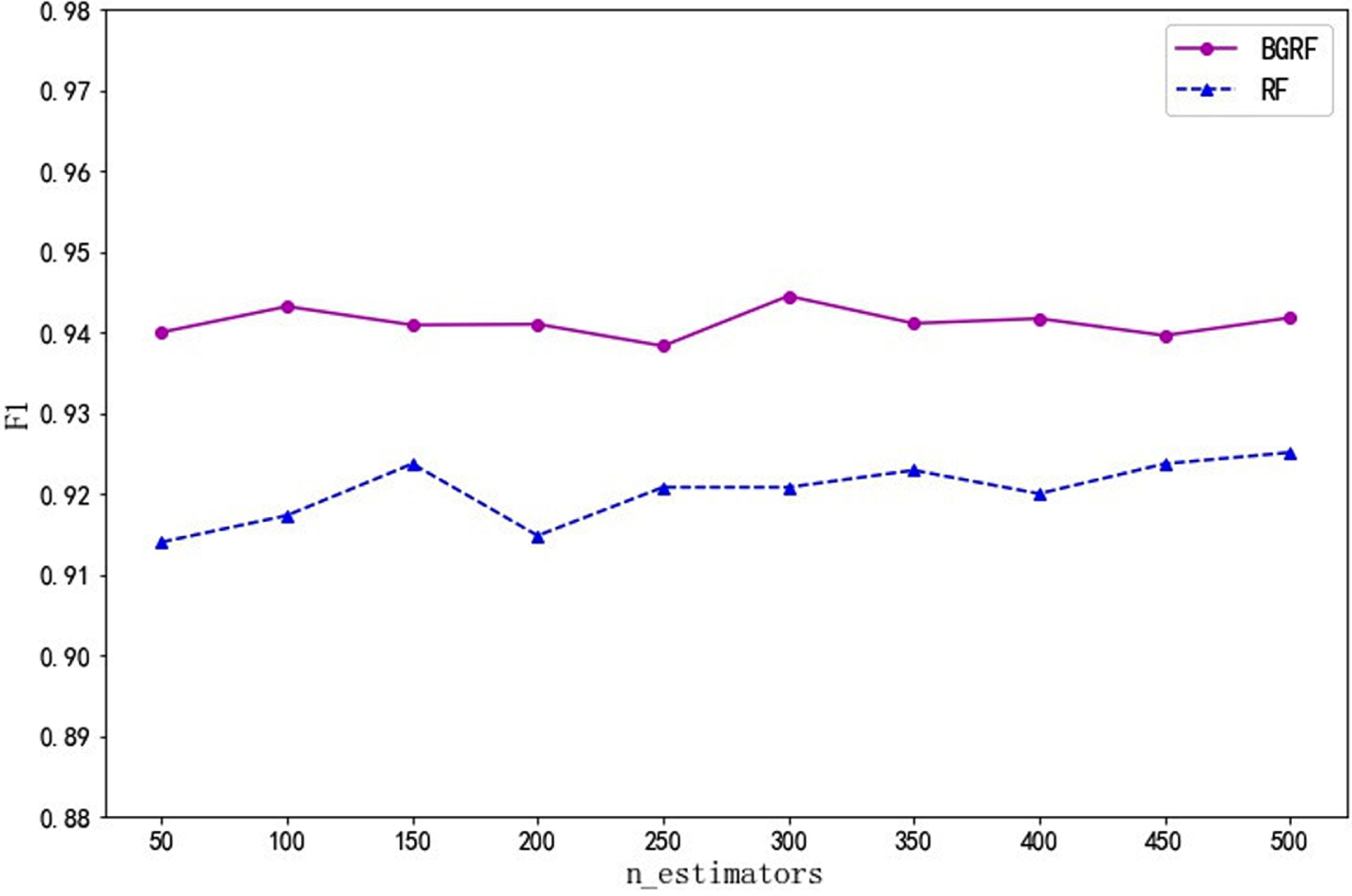
Fig. 4
F1 values of the data set Sonar on different numbers of trees.
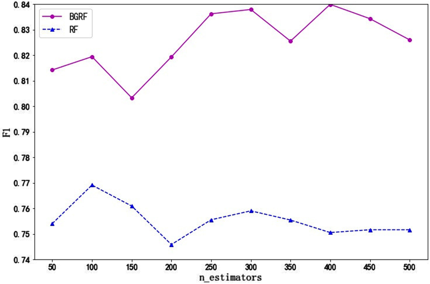
Fig. 5
The F1 values of the data set Heart on different numbers of trees.
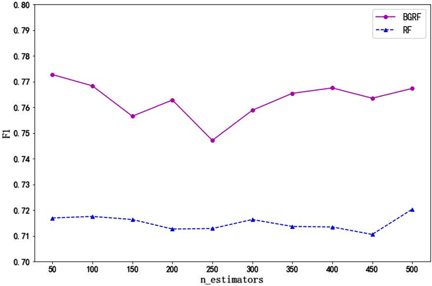
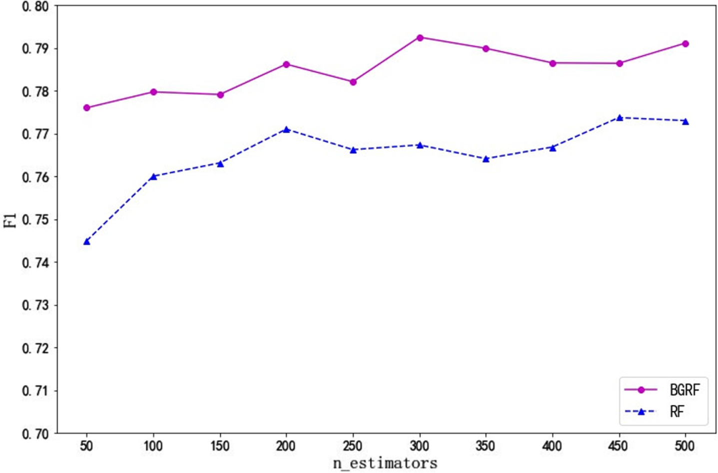
Fig. 6
The F1 values of the data set Bupa on different numbers of trees.
As can be seen from Fig. 3, for the Ionosphere data set, the F1 value of the BGRF algorithm is better than that of the RF algorithm. When the number of trees is 300, the maximum F1 value of the BGRF algorithm reaches 0.9445. When the number of trees is 500, the maximum F1 value of the RF algorithm reaches 0.9251. The BGRF algorithm improves the F1 value of the random forest by 2.10%.
As can be seen from Fig. 4, the F1 value of the BGRF algorithm is better than that of the RF algorithm for the Sonar data set. When the number of trees is 400, the maximum F1 value of the BGRF algorithm reaches 0.8399. When the number of trees is 150, the minimum F1 value of the BGRF algorithm is 0.8033. The change in the number of trees improves the F1 value of the BGRF algorithm by 4.56%. When the number of trees is 100, the maximum F1 value of the RF algorithm reaches 0.7691. The BGRF algorithm improves the F1 value of the random forest by 9.21%.
It can be seen from Fig. 5 that the F1 value of the BGRF algorithm is better than that of the RF algorithm for the Heart data set. The F1 value of the BGRF algorithm decreases and then increases with the number of trees. When the number of trees is 50, the maximum F1 value of the BGRF algorithm reaches 0.7727. When the number of trees is 250, the minimum F1 value of the BGRF algorithm is 0.7471. The change in the number of trees improves the F1 value of the BGRF algorithm by 3.43%. However, the RF algorithm is not sensitive to the change of the number of trees, and the fluctuation of the F1 value is small.
It can be seen from Fig. 6 that the F1 value of the BGRF algorithm is better than that of the RF algorithm for the Bupa data set. BGRF and RF algorithms show an overall upward trend. When the number of trees is 300, the maximum F1 value of the BGRF algorithm reaches 0.7927. When the number of trees is 250, the F1 value of the BGRF algorithm is 0.7821. When the number of trees is between 250 and 300, the BGRF algorithm improves the fastest by 1.36%.
The calculation method of the AUC value considers the classification ability of granular random forest for both positive and negative examples. In the case of unbalanced particles, it can still make a reasonable evaluation of the particle random forest. The classification results of the four UCI data sets evaluated by AUC values are shown in Figs. 7–10:
Fig. 7
AUC values for the dataset Ionosphere on different numbers of trees.
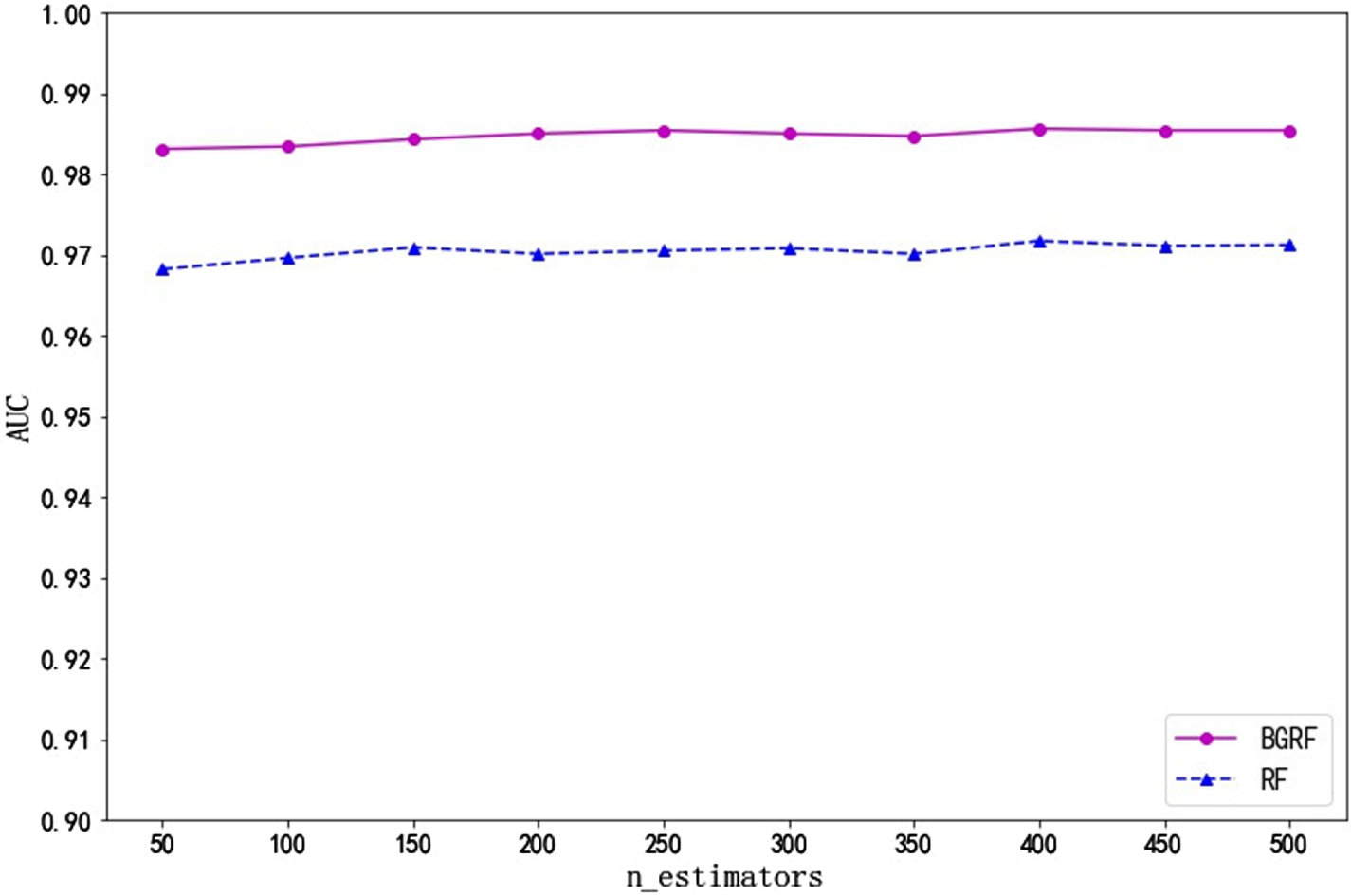
Fig. 8
AUC values for the data set Sonar on different numbers of trees.
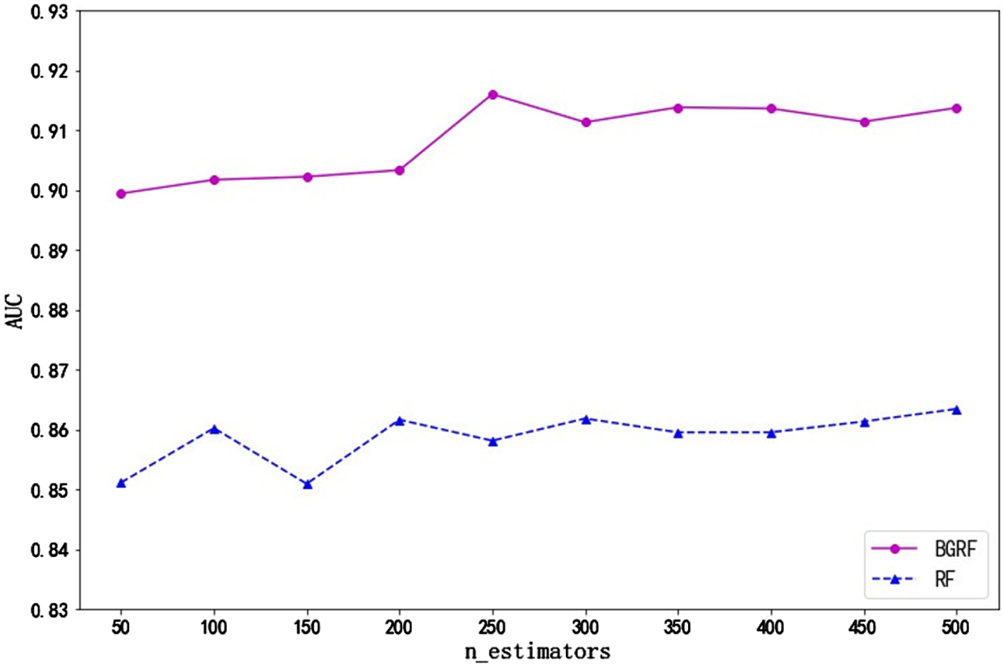
Fig. 9
AUC values for the data set Heart on different numbers of trees.
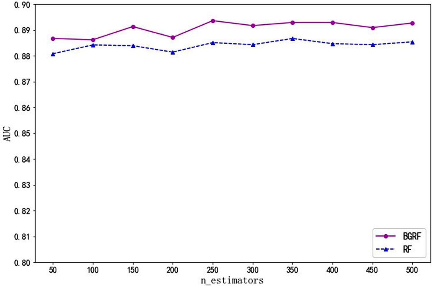
Fig. 10
AUC values for the data set Bupa on different numbers of trees.
It can be seen from Fig. 7 that the AUC value of the BGRF algorithm is better than that of the RF algorithm for the Ionosphere data set. When the number of trees is 400, the maximum AUC value of the BGRF algorithm reaches 0.9856. It shows that the BGRF model works very well. When the number of trees is 400, the maximum AUC value of the RF algorithm reaches 0.9717. The BGRF algorithm improves the AUC value of the random forest by 1.43%.
It can be seen from Fig. 8 that the AUC value of the BGRF algorithm is better than that of the RF algorithm for the Sonar data set. When the number of trees is 250, the maximum AUC value of the BGRF algorithm reaches 0.9160. When the number of trees is 50, the minimum AUC value of the BGRF algorithm is 0.8994. The change in the number of trees improves the F1 value of the BGRF algorithm by 1.85%. When the number of trees is 500, the maximum AUC value of the RF algorithm reaches 0.8634. The BGRF algorithm improves the AUC value of the random forest by 6.09%.
It can be seen from Fig. 9 that for the Heart data set, the AUC values of the BGRF and RF algorithms are close. But the AUC value of the BGRF algorithm is better than that of the RF algorithm. When the number of trees is 250, the maximum AUC value of the BGRF algorithm reaches 0.8936. The BGRF and RF algorithms are relatively stable concerning the number of trees.
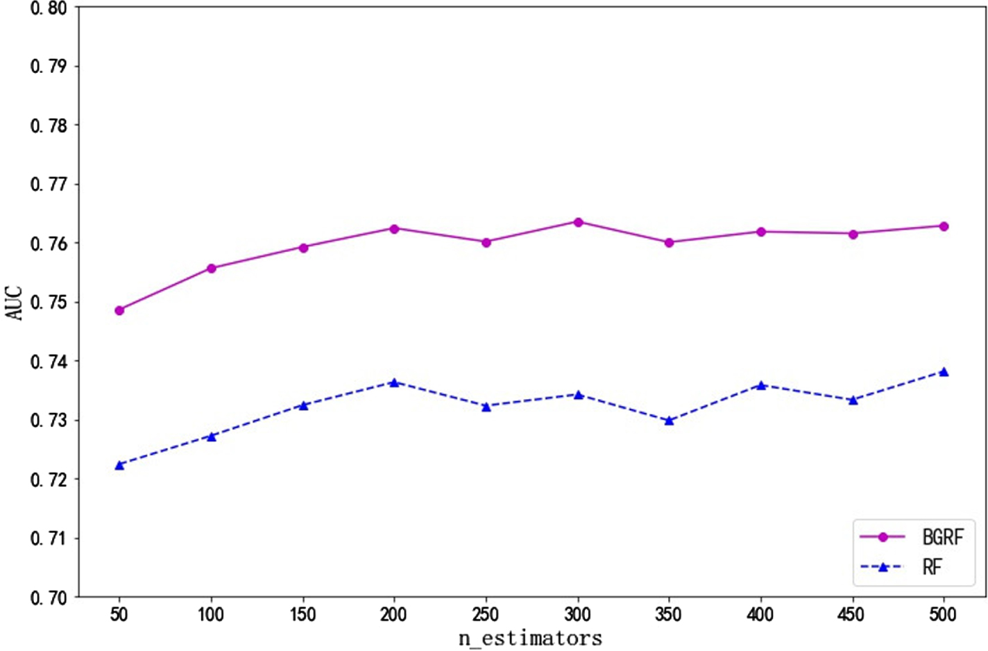
It can be seen from Fig. 10 that the AUC value of the BGRF algorithm is better than that of the RF algorithm for the Bupa data set. When the number of trees is 300, the maximum AUC value of the BGRF algorithm reaches 0.7635. When the number of trees is 500, the maximum AUC value of the RF algorithm reaches 0.7381. The BGRF algorithm improves the AUC value of the random forest by 3.44%.
From the experimental analysis of Figs. 3 to 10, it can be seen that the change in the number of trees has a greater impact on the F1 value. The BGRF algorithm is better than the RF algorithm under the evaluation index of F1 value and AUC value. The model of BGRF is more stable and can provide greater help for solving the binary classification problem. If too many or too few trees are selected, the fitting effect of the BGRF algorithm will be affected and the performance of the model will be reduced. Therefore, the classification effect of the BGRF algorithm can be improved by selecting the appropriate number of trees.
4.1.2Data visualization
In binary classification problems, the confusion matrix is a visual display tool to evaluate the quality of the binary classification model. Each column of the matrix represents the sample situation predicted by the model; each row of the matrix represents the real situation of the sample. The confusion matrix of BGRF is shown in Figs. 11–14.
Fig. 11
Confusion matrix of data set Ionosphere.
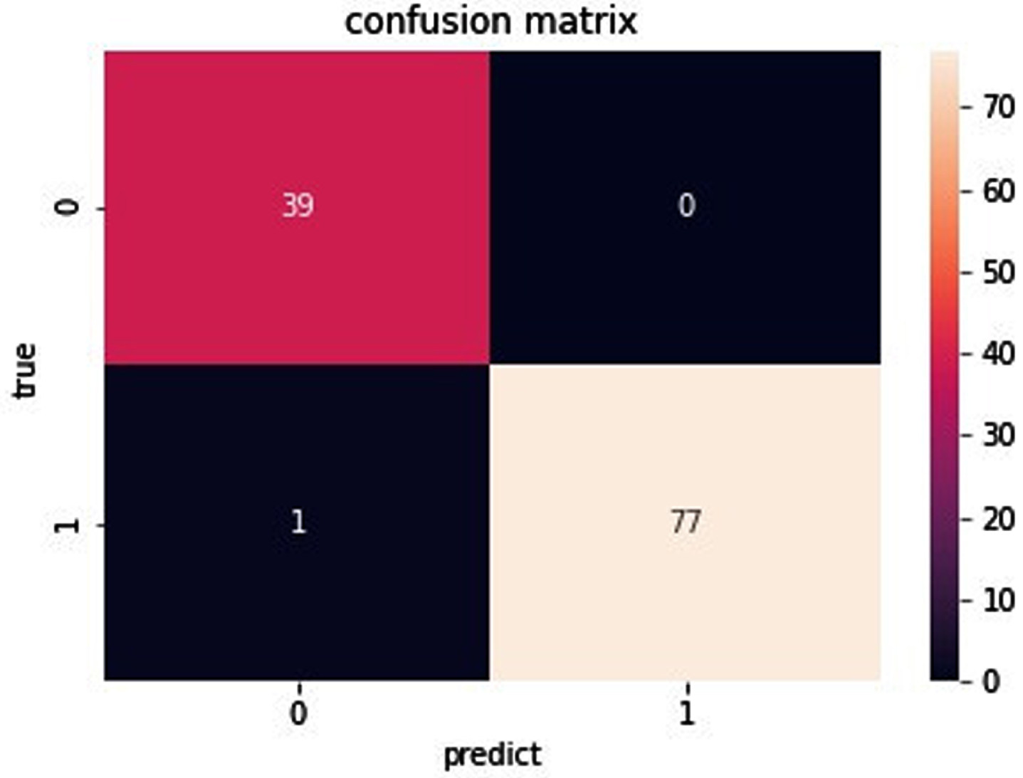
Fig. 12
Confusion matrix of data set Sonar.
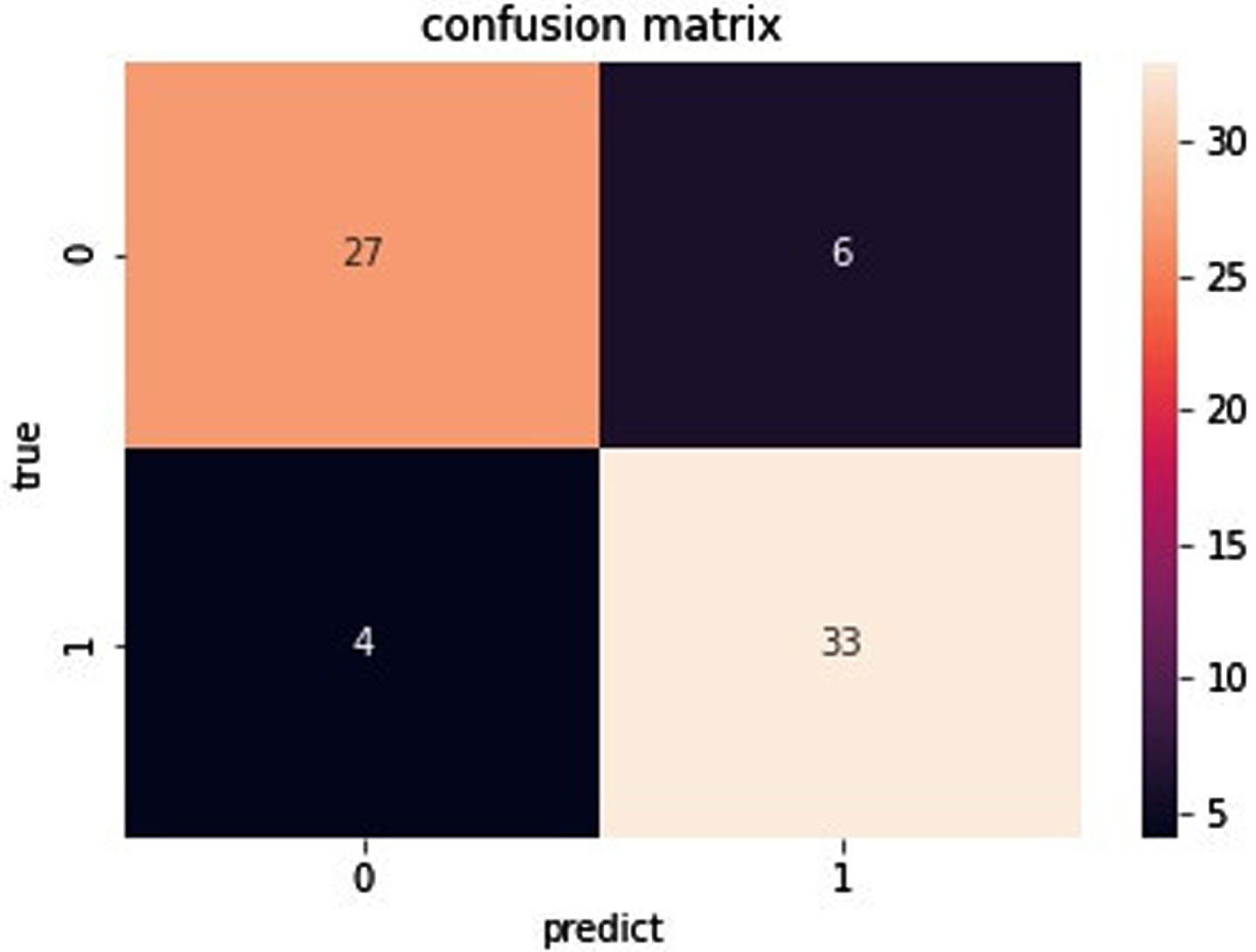
Fig. 13
Confusion matrix of data set Heart.
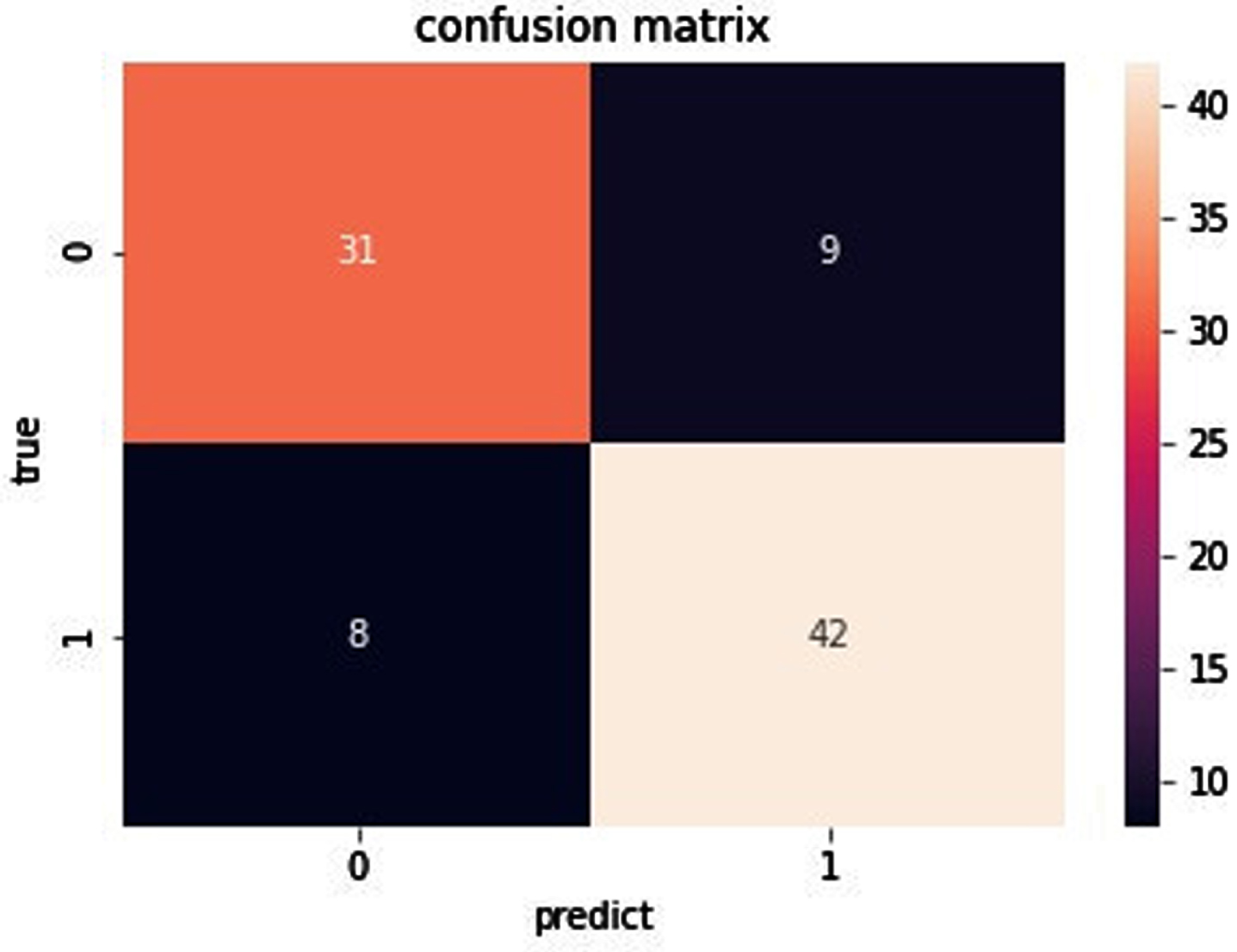
Fig. 14
Confusion matrix of data set Bupa.
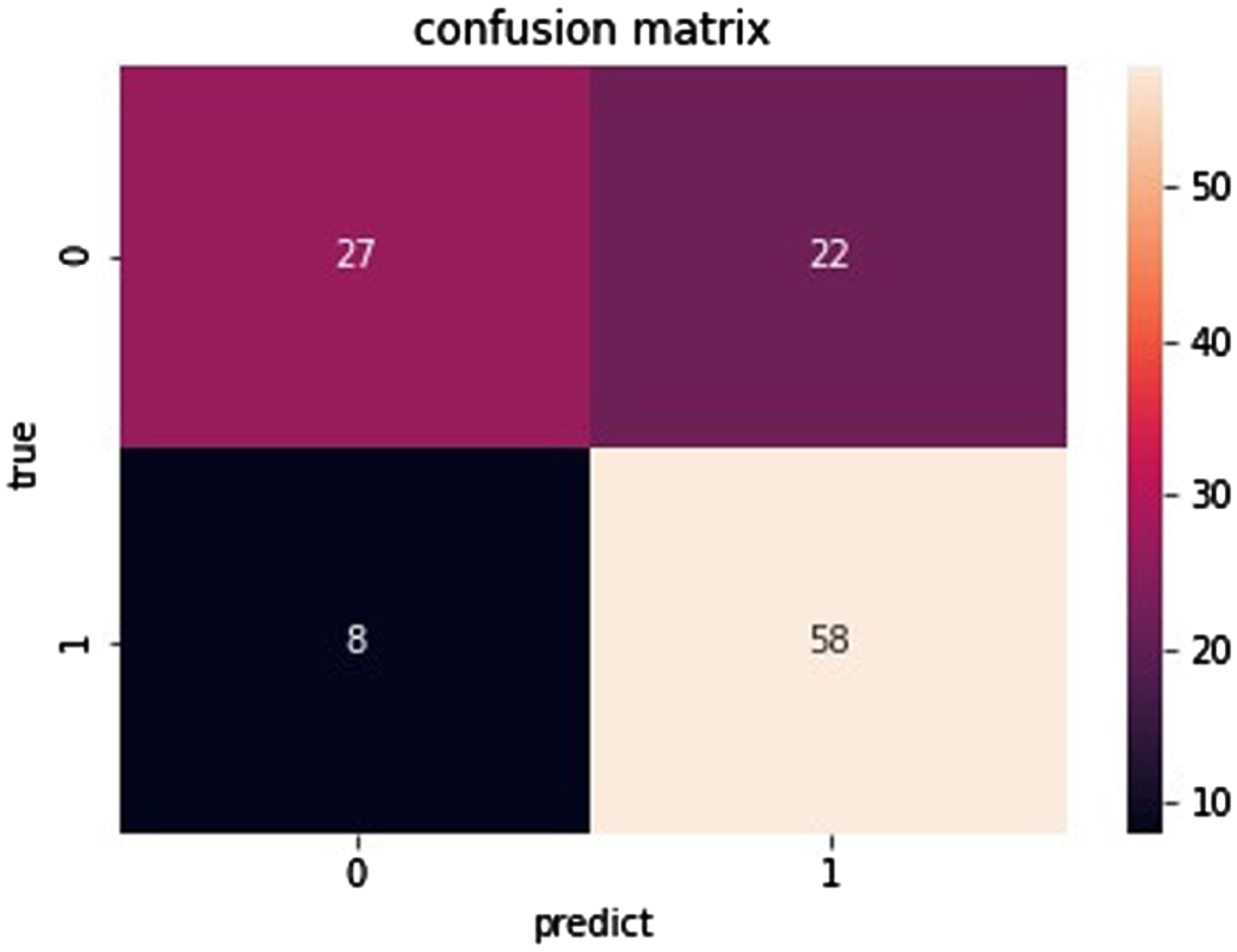
As you can see from Fig. 11, for the data set Ionosphere, the true positive is 39. The true negative is 77. The false negative is 0. The false positive is 1. As can be seen from Fig. 12, for the data set Sonar, the true positive is 27. The true negative is 33. The false negative is 6. The false positive is 4. As can be seen from Fig. 13, for the data set Heart, the true positive is 31. The true negative is 42. The false negative is 9. The false positive is 8. As can be seen from Fig. 14, for the data set Bupa, the true positive is 27. The true negative is 58. The false negative is 22. The false positive is 8. the BGRF has a high true positive and true negative. the BGRF has a low false negative and false positive. Therefore, the BGRF has better robustness.
The ROC curve is also a visualization method, and the ROC curve is used for visual discrimination through graphics. The area under the ROC curve is the AUC value. The ROC curves for the BGRF are shown in Figs. 15–18.
Fig. 15
ROC curve for the data set Ionosphere.
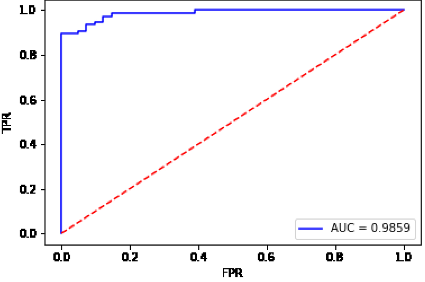
Fig. 16
ROC curve for the data set Sonar.
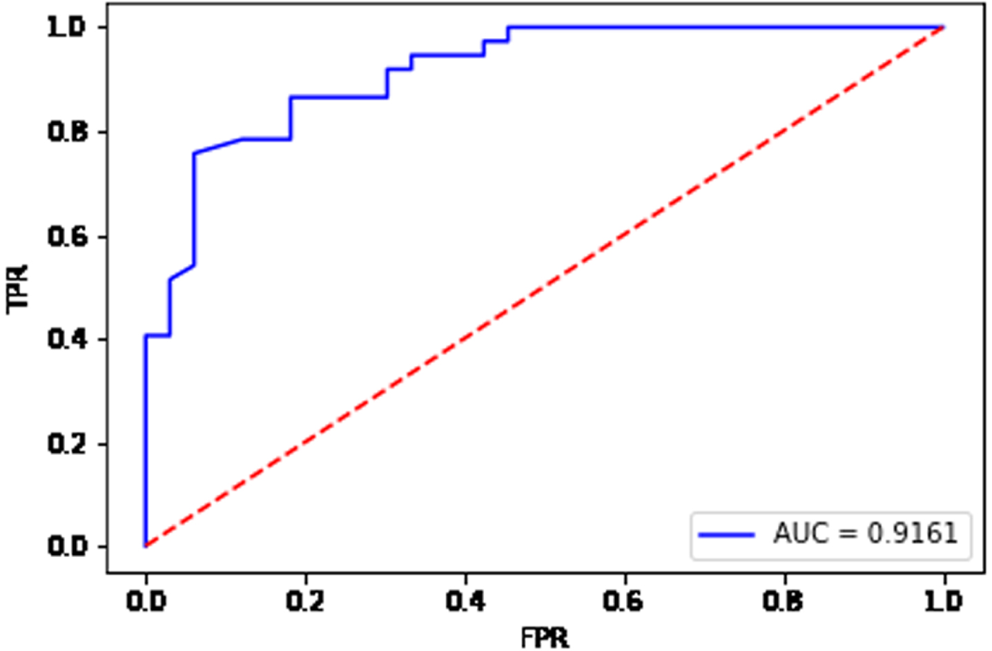
Fig. 17
ROC curve for the data set Heart.
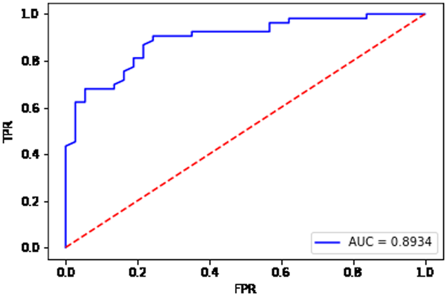
Fig. 18
ROC curve for the data set Bupa.
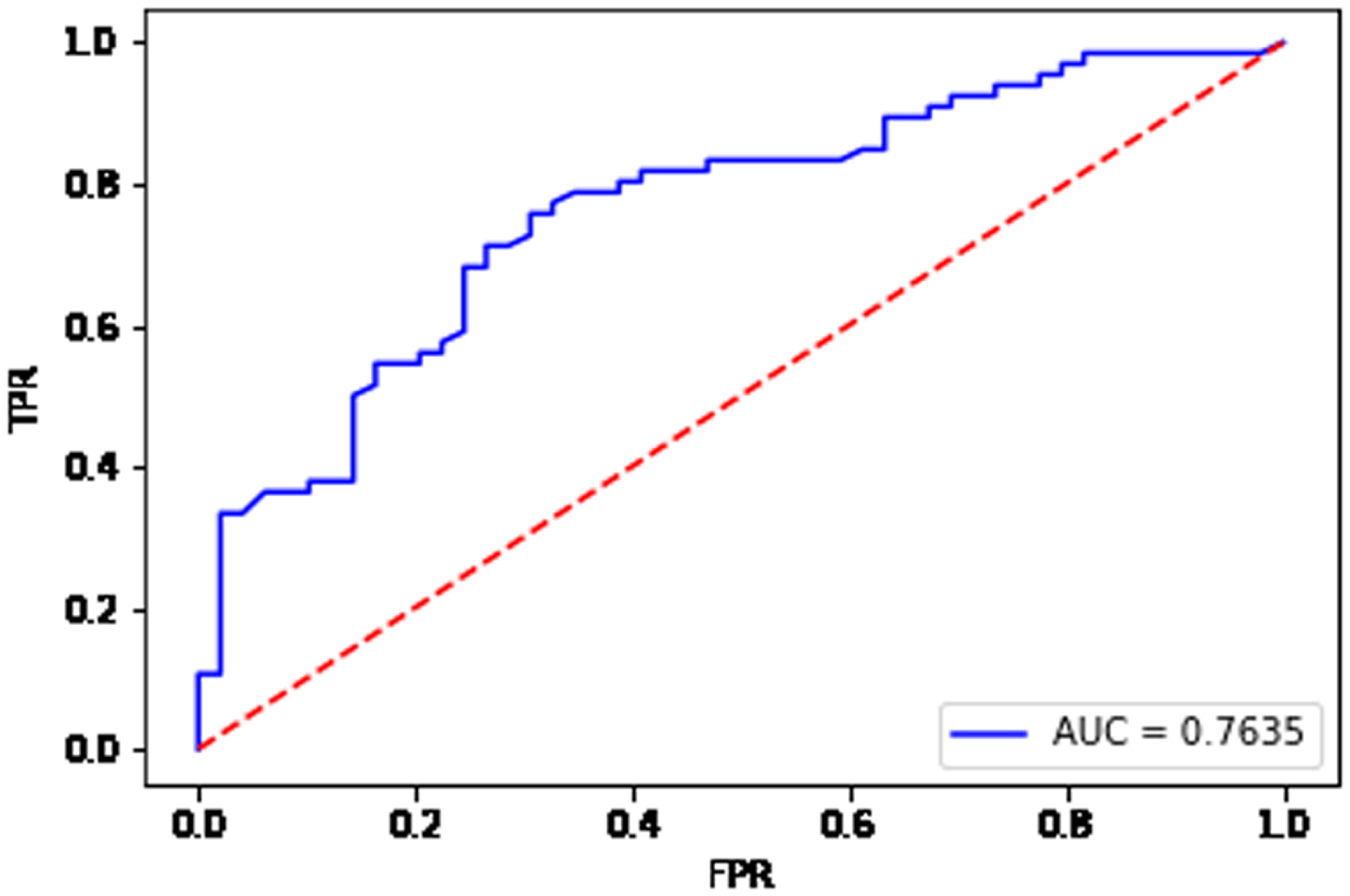
From Fig. 15, the AUC value is equal to 0.9859 for the data set Ionosphere. From Fig. 16, the AUC value is equal to 0.9161 for the data set Sonar. From Fig. 17, the AUC value is equal to 0.8934 for the data set Heart. From Fig. 18, the AUC value is equal to 0.7635 for the data set Bupa. The BGRF has a high AUC value. The ROC curve of the BGRF is closer to the upper left corner. Therefore, the BGRF is a relatively stable classifier.
4.1.3Comparison of traditional algorithms
The number of trees in a granular random forest affects the classification performance of a granular classifier. The experiment in this section mainly compares the difference between the granular random forest and the traditional classification algorithm under different evaluation indexes. The number of trees in the forest is selected as the number with the best classification effect in the experiment in Section 4.1.1. The classification results of the four UCI data sets are shown in Tables 3 and 4.
Table 3
Comparison of the results of each algorithm on different data sets with F1 value as the performance evaluation
| Data sets | BGRF | CART | RF | GBDT | LR | KNN | SVM |
| Ionosphere | 0.9445 | 0.9093 | 0.9251 | 0.9305 | 0.9032 | 0.8805 | 0.9342 |
| Sonar | 0.8399 | 0.7251 | 0.7691 | 0.7437 | 0.7467 | 0.7632 | 0.8056 |
| Heart | 0.7727 | 0.6212 | 0.7203 | 0.7222 | 0.7429 | 0.7429 | 0.7429 |
| Bupa | 0.7925 | 0.7211 | 0.7737 | 0.7124 | 0.7356 | 0.6809 | 0.7532 |
Table 4
Comparison of the results of each algorithm on different data sets with AUC value as the performance evaluation
| Data sets | BGRF | CART | RF | GBDT | LR | KNN | SVM |
| Ionosphere | 0.9856 | 0.8811 | 0.9717 | 0.9627 | 0.8798 | 0.8594 | 0.9686 |
| Sonar | 0.9160 | 0.6802 | 0.8634 | 0.8563 | 0.8106 | 0.8805 | 0.8850 |
| Heart | 0.8936 | 0.6815 | 0.8867 | 0.8646 | 0.8718 | 0.8175 | 0.8766 |
| Bupa | 0.7635 | 0.6488 | 0.7381 | 0.7000 | 0.6652 | 0.5986 | 0.7078 |
It can be seen from Table 3 that in the data set Ionosphere, the SVM has the largest F1 value of 0.9342 in the traditional algorithm, while the F1 value of the BGRF is 0.9445. In the data set Sonar, the SVM has the largest F1 value of 0.8056 in the traditional algorithm, while the F1 value of the BGRF is 0.8399. In the data set Heart, the LR, KNN, and SVM have the largest F1 value of 0.7429 in the traditional algorithm, while the F1 value of the BGRF is 0.7727. In the data set Bupa, the RF has the largest F1 value of 0.7737 in the traditional algorithm, while the F1 value of the BGRF is 0.7925. The BGRF algorithm has a larger F1 value than the traditional algorithm on the Ionosphere, Sonar, Hear, and Bupa data sets [36]. It shows that the BGRF algorithm has better binary classification performance than the traditional algorithm on these data sets. In the comparison of the experimental results of the Ionosphere data set, it can be seen that the BGRF algorithm has the maximum value in the F1 evaluation index. The results show that the BGRF algorithm has the highest harmonic average of precision and recall, and has the best binary classification effect.
It can be seen from Table 4 that the AUC value of RF in the traditional algorithm is the highest on the Ionosphere, Heart, and Bupa data sets. But the RF algorithm is slightly low than the BGRF algorithm proposed in this pap. On the Sonar data set, the AUC value of SVM is the highest among the traditional algorithms. However, the AUC value of the BGRF algorithm is 0.031 higher than that of SVM. On the whole, the performance of the proposed BGRF algorithm is better than the other six traditional algorithms. The higher the AUC of the BGRF algorithm is, the better the binary classification model is.
In general, the BGRF classification algorithm proposed in this paper has a better binary classification effect and a more stable binary classification model on each standard data sets.
4.2Multi-classification experiments
4.2.1Number of trees affects
Accuracy is a common evaluation index for multi-classification. The accuracy rate is well understood, the number of correctly predicted samples divided by the total number of samples. The classification results of the four UCI data sets evaluated by accuracy are shown in Figs. 19–22:
Fig. 19
Accuracy of data set Vowel on different numbers of trees.
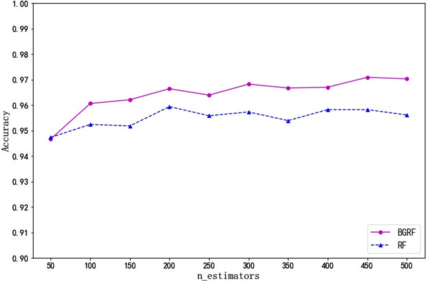
Fig. 20
Accuracy of the data set Newthyroid over different numbers of trees.
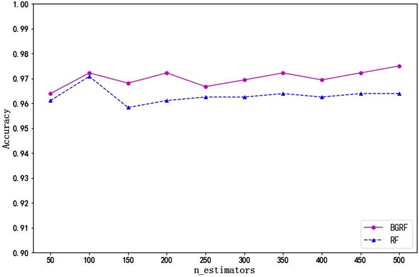
Fig. 21
Accuracy of the data set Ecoli over different numbers of trees.
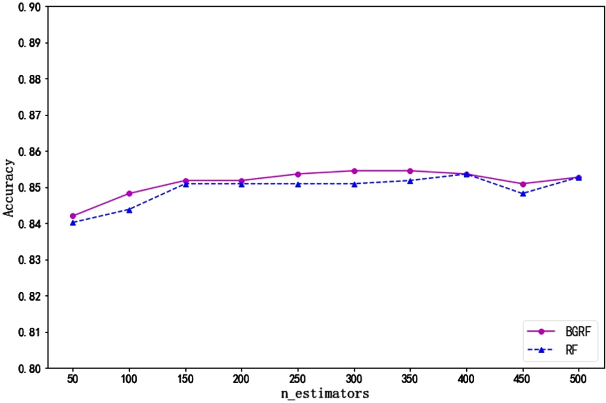
Fig. 22
Accuracy of Data Set Glass on different numbers of trees.
As can be seen from Fig. 19, for the Vowel data set, the RF algorithm is higher than the BGRF algorithm only once. When the number of trees is greater than 50, the BGRF algorithm outperforms the RF algorithm. When the number of trees is 450, the maximum accuracy of the BGRF algorithm reaches 0.9709. It shows that the classification effect of the BGRF model is very good. The accuracy of the BGRF algorithm is 0.9467 when the number of trees is 50. As the number of trees changes, the BGRF algorithm improves its accuracy by 2.56%.
It can be seen from Fig. 20 that the accuracy of the BGRF algorithm is better than that of the RF algorithm for the Newthyroid data set. When the number of trees is 500, the maximum accuracy of the BGRF algorithm reaches 0.9750. It is shown that the BGRF algorithm is suitable for this classification. When the number of trees is 100, the maximum accuracy of the RF algorithm reaches 0.9708. When the number of trees is 100, the RF algorithm has reached its maximum and cannot continue to increase accuracy by changing the number of trees.
As can be seen from Fig. 21, for the Ecoli data set, the RF algorithm has only one higher accuracy than the BGRF algorithm. When the number of trees is 350, the maximum accuracy of the BGRF algorithm reaches 0.8545. When the number of trees is 400, the maximum accuracy of the RF algorithm reaches 0.8536, and the RF algorithm is higher than the BGRF algorithm only once. The accuracy curves of the BGRF and Random Forest are similar, but the BGRF is slightly better than RF.
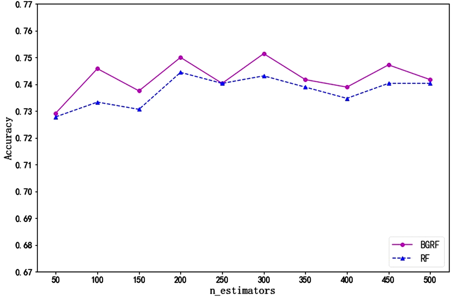
It can be seen from Fig. 22 that for the Glass data set, the accuracy of the RF algorithm is equal to that of the BGRF algorithm only once. When the number of trees is 300, the maximum accuracy of the BGRF algorithm reaches 0.7514. When the number of trees is 250, the accuracy of the RF algorithm is equal to the BGRF algorithm. In general, the BGRF algorithm is slightly better than the RF algorithm.
From the experimental analysis of Figs. 19 to 22, it can be seen that the change in the number of trees will affect accuracy. The BGRF algorithm is slightly better than the RF algorithm under the evaluation index of accuracy. In the multi-classification problem, the BGRF model needs to choose the appropriate number of trees to improve the accuracy of the algorithm.
4.2.2Comparison of traditional algorithms
The number of trees in the forest is selected as the value with the best classification effect in the experiment in Section 4.2.1. The classification results of the four UCI data sets are shown in Table 5.
Table 5
Comparison of the results of each algorithm on different data sets with accuracy as the performance evaluation
| Data sets | BGRF | CART | RF | GBDT | LR | KNN | SVM |
| Vowel | 0.9709 | 0.7915 | 0.9594 | 0.8561 | 0.5242 | 0.8000 | 0.8394 |
| Newthyroid | 0.9750 | 0.9222 | 0.9708 | 0.9444 | 0.8194 | 0.8889 | 0.9167 |
| Ecoli | 0.8545 | 0.8241 | 0.8536 | 0.8045 | 0.7857 | 0.8304 | 0.8393 |
| Glass | 0.7514 | 0.6583 | 0.7444 | 0.6778 | 0.5833 | 0.5694 | 0.6806 |
It can be seen from Table 5 that in the comparison of the experimental results of the Newthyroid data set, the BGRF algorithm has the maximum value in terms of the accuracy evaluation index. On the four datasets, the BGRF algorithm proposed in this paper has a slight improvement in accuracy compared with the other six traditional algorithms. The results show that the BGRF algorithm is very close to the true value.
In general, the classification accuracy of the BGRF classification algorithm proposed in this paper is relatively high on each standard data set. The broad granular random forest algorithm is different from the traditional algorithm. The BGRF algorithm uses width granulation technology to improve the structure so that the data can better meet the requirements of the algorithm. The BGRF algorithm improves the classification performance of the algorithm so that the algorithm can be compatible with more types of data sets. The BGRF has good AUC and F1 values in binary classification problems, so the BGRF is robust. In multi-classification problems, the BGRF has better accuracy, so the BGRF has scalability.
5Conclusion
To improve the performance of random forests in dealing with classification problems, a broad granular random forest algorithm is proposed in this paper. The algorithm introduces the broad granulation method to construct the broad granules and the broad granular vectors in the data sets system. The decision rule of the broad granules is defined, and the broad granular vectors are applied. A granular decision tree is designed to effectively improve the overall classification performance of the granular random forest. The method of width granulation is an improved strategy for the granular classifier. It can enhance the classification performance of the original algorithm when it is applied to the random forest algorithm.
The broad granular random forest algorithm proposed in this paper has good accuracy in dealing with multi-classification problems. In addition, the BGRF also has better classification performance for binary classification problems, and the BGRF improves the AUC value and F1 value. The BGRF is good at working with collection-type data. However, the BGRF is not suitable for processing image and video data. In future work, the granulation method will be improved. Combining the granulation method with the neighborhood rough set, a new granulation method is proposed to generate granules that are more suitable for the classifier. In future work, a new granular classifier is designed as the base classifier to improve the robustness and flexibility of the ensemble model. Future research will focus on the classification of real complex data, and further expand the scope of application of broad granular random forest.
Acknowledgments
This work is supported by the National Natural Science Foundation of China (No. 61976183) and the Joint Project of Production, Teaching and Research of Xiamen (No. 2022CXY04028).
References
[1] | Subudhi S. and Panigrahi S. , Application of OPTICS and ensemblelearning for Database Intrusion Detection, Journal of King SaudUniversity-Computer and Information Sciences 34: (3) ((2022) ), 972–981. |
[2] | Ahmadi A. , Nabipour M. , Mohammadi-Ivatloo B. and VahidinasabEnsemble V. , learning-based dynamic line rating forecasting undercyberattacks, IEEE Transactions on Power Delivery 37: (1) ((2022) ), 230–238. |
[3] | Kamble K.S. , Sengupta J. and Kamble K. , Ensemble machinelearning-based affective computing for emotion recognition usingdual-decomposed EEG signals, IEEE Sensors Journal 22: (3) ((2022) ), 2496–2507. |
[4] | Yang X. , Xu Y. , Quan Y. and Ji H. , Image denoising via sequentialensemble learning,, IEEE Transactions on Image Processing 29: ((2020) ), 5038–5049. |
[5] | Zhang X. , Nojima Y. , Ishibuchi H. , Hu W. and Wang S. , Prediction byfuzzy clustering and KNN on validation data with parallel ensembleof interpretable TSK fuzzy classifiers, IEEE Transactions onSystems Man Cybernetics-Systems 52: (1) ((2022) ), 400–414. |
[6] | Breiman L. , Random forests, Machine learning 45: (1) ((2001) ), 5–32. |
[7] | Breiman L. , Bagging predictors, Machine learning 24: (2) ((1996) ), 123–140. |
[8] | Yates D. and Islam M.Z. , FastForest: Increasing random forestprocessing speed while maintaining accuracy, InformationSciences 557: ((2021) ), 130–152. |
[9] | Sun J. , Yu H. , Zhong G. , Dong J. , Zhang S. and Yu H. , Random shapleyforests: cooperative game-based random forests with consistency, IEEE Transactions on Cybernetics 52: (1) ((2022) ), 205–214. |
[10] | Han S. , Kim H. and Lee Y. , Double random forest, Machinelearning 109: (8) ((2020) ), 1569–1586. |
[11] | Su L. , Huang S. , Wang Z. , Zhang Z. , Wei H. and Chen T. , Whole slidecervical image classification based on convolutional neural networkand random forest, International Journal of Imaging Systems andTechnology 32: (3) ((2022) ), 767–777. |
[12] | Chen L. , Su W. , Feng Y. , Wu M. , She J. and Hirota K. , Two-layerfuzzy multiple random forest for speech emotion recognition inhuman-robot interaction, Information Sciences 509: (2020), 150–163. |
[13] | Wei Y. , Yang Y. , Xu M. and Huang W. , Intelligent fault diagnosis ofplanetary gearbox based on refined composite hierarchical fuzzyentropy and random forest, ISA Transactions 109: ((2021) ), 340–351. |
[14] | Liu Z. , Siu W. and Chan Y. , Features guided face super-resolutionvia hybrid model of deep learning and random forests, IEEETransactions on Image Processing 30: ((2021) ), 4157–4170. |
[15] | Yu Z. , Zhang C. , Xiong N. and Chen F. , A new random forest appliedto heavy metal risk assessment, Computer Systems Science andEngineering 40: (1) ((2022) ), 207–221. |
[16] | Pavlov Y.L. , The maximum tree of a random forest in theconfiguration graph, Sbornik Mathematics 212: (9) ((2021) ), 1329–1346. |
[17] | Zadeh L.A. , Toward a theory of fuzzy information granulation and itscentrality in human reasoning and fuzzy logic, Fuzzy Sets andSystems 90: (2) ((1997) ), 111–127. |
[18] | Yao J.T. , Vasilakos A.V. and Pedrycz W. , Granular computing:perspectives and challenges, IEEE Transactions on Cybernetics 43: (6) ((2013) ), 1977–1989. |
[19] | Pan L. , Gao X. , Deng Y. and Cheong K.H. , Constrained pythagoreanfuzzy sets and its similarity measure, IEEE Transactions onFuzzy Systems 30: (4) ((2022) ), 1102–1113. |
[20] | Niu J. , Chen D. , Li J. and Wang H. , Fuzzy rule-based classificationmethod for incremental rule learning, IEEE Transactions onFuzzy Systems 30: (9) ((2022) ), 3748–3761. |
[21] | Xia S. , Zhang H. , Li W. , Wang G. , Giem E. and Chen Z. , GBNRS: Anovel rough set algorithm for fast adaptive attribute reduction inclassification, IEEE Transactions on Knowledge and DataEngineering 34: (3) ((2022) ), 1231–1242. |
[22] | Xie X. , Zhang X. and Zhang S. , Rough set theory and attributereduction in interval-set information system, Journal ofIntelligent & Fuzzy Systems 42: (6) ((2022) ), 4919–4929. |
[23] | Mi Y. , Liu W. , Shi Y. and Li J. , Semi-supervised concept learning byconcept-cognitive learning and concept space, IEEE Transactionson Knowledge and Data Engineering 34: (5) ((2022) ), 2429–2442. |
[24] | Zhang T. , Liu M. and Rong M. , Attenuation characteristics analysisof concept tree, Journal of Intelligent & Fuzzy Systems 39: (3) ((2020) ), 4081–4094. |
[25] | Shen F. , Zhang X. , Wang R. , Lan D. and Zhou W. , Sequentialoptimization three-way decision model with information gain forcredit default risk evaluation, International Journal ofForecasting 38: (3) ((2022) ), 1116–1128. |
[26] | Peng J. , Cai Y. , Xia G. and Hao M. , Three-way decision theory basedon interval type-2 fuzzy linguistic term sets, Journal ofIntelligent & Fuzzy Systems 43: (4) ((2022) ), 3911–3932. |
[27] | Zhang Y. , Zhao T. , Miao D. and Pedrycz W. , Granular multilabel batchactive learning with pairwise label correlation, IEEETransactions on Systems Man Cybernetics-Systems 52: (5) ((2022) ), 3079–3091. |
[28] | Fu S. , Wang G. , Xu J. and Xia S. , IbLT: An effective granulmputing framework for hierarchical community detection, Journal of Intelligent Information Systems 58: (1) ((2022) ), 175–196. |
[29] | Wei W. , Wang D. and Liang J. , Accelerating ReliefF using informationgranulation, International Journal of Machine Learning andCybernetics 13: (1) ((2022) ), 29–38. |
[30] | Wang Y. , Hu Q. , Chen H. and Qian Y. , Uncertainty instructedmulti-granularity decision for large-scale hierarchicalclassification, Information Sciences 586: ((2022) ), 644–661. |
[31] | Huang Y. , Li T. , Luo C. , Fujita H. and Horng S. , Dynamic fusion ofmultisource interval-valued data by fuzzy granulation,, IEEETransactions on Fuzzy Systems 26: (6) ((2018) ), 3403–3417. |
[32] | Shah N. , Ali M.I. , Shabir M. , Ali A. and Rehman N. , Uncertaintymeasure of Z-soft covering rough models based on a knowledgegranulation, Journal of Intelligent & Fuzzy Systems 38: (2) ((2020) ), 1637–1647. |
[33] | Chen Y. , Qin N. , Li W. and Xu F. , Granule structures, distances andmeasures in neighborhood systems, Knowledge-based Systems 165: ((2019) ), 268–281. |
[34] | Jiang H. , Chen Y. , Kong L. , Cai G. and Jiang H. , An LVQ clusteringalgorithm based on neighborhood granules, Journal ofIntelligent & Fuzzy Systems 43: (5) ((2022) ), 6109–6122. |
[35] | Chen C.L.P. and Liu Z. , Broad learning system: an effective andefficient incremental learning system without the need for deeparchitecture, IEEE Transactions on Neural Networks and LearningSystems 29: (1) ((2018) ), 10–24. |
[36] | Dua D. , Graff C. UCI Machine Learning Reposi-tory [http://archive.ics.uci.edu/ml] Irvine, CA: University of California, School of Information and Computer Science (2019). |

