


Introduction
The Steele Glacier is a large valley glacier in the St Elias Mountains, Yukon Territory, Canada. Explorations by Reference WoodWood (1936) and Reference SharpSharp (1951) indicate that for at least thirty years prior to 1965, the 10–15 km lower zone was inactive and provided a safe, relatively uncrevassed route into the Icefield Ranges. Austin Post finds photographic evidence for “an extensive surge which severely fractured the surface of the upper glacier” around 1940 and “must have faded out near the ‘big bend’ of the Steele”, some 12 km from the present terminus (personal communication from M. F. Meier). By summer 1966 Steele Glacier was in the midst of a spectacular surge which displaced surface features 8 km within one year. Premonitory signs, apparent on aerial photographs, led Post in 1960 to predict the Steele’s surge, but unfortunately none witnessed the onset of the active phase. Reference StanleyStanley (1969) and Meier (personal communication) refer to aerial photographs, taken by Post in the summer of 1965, which show extensive crevassing of the glacier surface, and indicate the advance probably began in 1965. From August 1966 the surge is well documented (Reference BayrockBayrock, 1967; Reference StanleyStanley, 1969; Reference WoodWood, 1967[a], Reference Wood[b]; Reference Thomson, Bushnell and RagleThomson, 1972) and Reference Wood, Bushnell and RagleWood (1972) has published an historical review containing striking pre-surge and post-surge photographs.
The cause of the Steele surge is unknown, but as the nearby Rusty and Trapridge Glaciers appear to surge by a thermal instability mechanism, temperature measurements in Steele Glacier could prove diagnostic. Consequently in July 1972 a reconnaissance program of ice-temperature measurement was begun and a single hole was thermally drilled to a depth of 114 m in the central region of the glacier (Fig. 1). Two eight-conductor cables attached to the power cable of the thermal probe carried thirteen calibrated thermistors to depths ranging from 25 m to 114 m. The drilling and temperature measurement procedures were essentially the same as those described by Classen and Reference Classen, Clarke, Bushnell and RagleClarke (1972). Thermistor resistances were measured ten days after the termination of drilling and converted to ice temperatures.
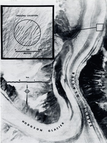
Fig. 1. Portion of Canadian Government air photograph A21523-73 showing confluence region of Steele and Hodgson Glaciers. Inset shows details of crevasses near drilling site.
Cooling curves obtained from holes drilled with thermal probes of various diameters on the nearby Trapridge Glacier show that thermal equilibrium is not reached in ten days. To correct the measured temperatures, theoretical cooling curves were computed. The diffusion equation was solved in cylindrical polar coordinates, by finite-difference methods, for a water-filled cylindrical hole in cold ice (Appendix A). The solution yields both hole closure and ice temperature as a function of time, and the resulting cooling curves can be compared to observational data if the initial hole radius is known. The thermal probe radius is not a good estimate of the initial hole radius because the probe efficiency is not 100%. A better estimate of this radius is obtained by assuming that all the thermal energy from the probe is used to melt ice. For drilling speed v p the radius of the hole r c can be calculated as
where P is the input power to the probe, L the latent heat of fusion (3.337 × 10⁵ J/kg), and ρ the ice density. As both P and v p were monitored continuously during field operations, the appropriate values of r c can be computed at each thermistor depth, P and v p did not change rapidly with probe depth so that in the neighbourhood of each thermistor the hole was nearly cylindrical with r c given by Equation (1). Comparisons of theoretical cooling curves and data recorded at three sites on Trapridge Glacier (Jarvis, unpublished) show good agreement, and the corrected Steele Glacier temperatures are expected to be within ±0.2° C of the true equilibrium values. The observed ten-day temperatures and the values corrected to equilibrium are given in Table 1.
Table I. Steele Glacier Temperature Data

In the region of the drill site, the upper 114 m of the glacier is cold but the temperature profile is unusual and unexpected. Below 50 m the ice cools with depth suggesting the presence of a heat source near 40 m. No similar anomaly has been observed on the nearby Rusty and Trapridge Glaciers, two surge-type glaciers in the quiescent phase (Reference Classen and ClarkeClassen and Clarke, 1971; Clarke and Goodman, in press; Jarvis and Clarke, unpublished). Geothermal heat causes the temperature in these cold glaciers to increase with depth. Thus the anomaly does not appear to reflect a regional climatic amelioration but is probably a consequence of the Steele Glacier’s most recent surge. The ice thickness is thought to be considerably greater than 114 m, so a continued temperature decrease to the glacier bed seems unlikely. If one makes the reasonable assumption that prior to the surge the temperature increased monotonically with depth, the upper 114 m must have been colder than –6.5° C before the advance began. Measurements on the Rusty and Trapridge Glaciers suggest that –8.0° C is a good estimate of the mean annual surface temperature.
The apparent heat source near 40 m must be localized in the vertical sense and be of sufficient strength to have maintained the observed anomaly for the six or seven years since the surge onset. Available energy sources are internal viscous heating, friction from sliding along shear planes, and internal water cavities. Thermal anomalies might also be generated by advective heat transfer or large displacements along shear planes. Viscous heating and sliding friction are insufficient to produce the observed effect. Aerial photographs analyzed by Reference StanleyStanley (1969) show that the drill site was in a zone of surface lowering and active extensional flow throughout the surge so that neither advection nor ice displacement along shear planes could account for the anomalously warm temperatures near 40 m. (Even in a region of passive compressive flow a temperature anomaly of 6.0° C would require an unreasonably large upward mass transport.) We therefore conclude that englacial water cavities are the most probable energy source.
During the Steele Glacier surge, crevasses as wide as 20 m and as deep as 100 m were not uncommon. Since extensive crevassing reduces albedo and inhibits surface run-off, large quantities of melt-water can enter newly formed crevasses and gain access to considerable depths within the glacier. Collins (Reference NielsenNielsen, 1969, discussion on p. 960) remarked that this should have a noticeable effect on the temperature of a cold surge-type glacier and speculated that on some surging glaciers water might even be admitted to the glacier bed. Our observations support the first suggestion but not the latter.
Crevasse model
To evaluate the thermal effects of trapped water in a cold crevassed glacier, a twodimensional, time-dependent numerical model was developed. The ice temperature T was assumed to be a function of the space variables x, measured in the direction of flow, and y, the depth measured perpendicular to the glacier surface. Prior to the surge onset at t = 0 the glacier surface was assumed to be a plane maintained at a temperature which varied sinusoidally with time. (As might be expected the time-dependence of the surface boundary condition played a negligible role in the final results except near the surface–air boundaries.) The temperature at a depth d* far below the glacier surface was held constant at T d. Therefore the pre-surge temperature profile is linear with depth except near the glacier surface, and the temperature gradient is simply the apparent geothermal gradient.
At the surge onset, severe crevassing of the upper surface occurs, allowing melt water to partially fill the crevasses. Both the crevasse formation and water filling were assumed to occur instantaneously at t = 0. This assumption is justified if one is interested in ice temperatures several years after the surge has terminated. By that time the exact details of crevasse formation and water filling have an insignificant effect on the observed temperatures. For simplicity the crevasse field was assumed to be spatially periodic with infinitely long, symmetric crevasses at constant separation (Fig. 2). The initial shape of each crevasse was taken as a triangular wedge, although freezing of the trapped water modified the cross section with time. These assumptions yield a high degree of symmetry and it is only necessary to calculate the ice temperatures within the shaded region of Figure 2 to obtain the complete temperature solution.

Fig. 2. Model of crevasse field. Owing to spatial periodicity temperatures need only be evaluated in the shaded region.
Because the crevasses are assumed to contain water, the usual arguments predicting maximum crevasse depths based on creep rates do not apply (Reference WeertmanWeertman, 1971). When the crevasse is open at the surface, hydrostatic pressure of the trapped water resists creep closure; when it is sealed by surface freezing, incompressibility of the water cavity prevents creep closure entirely so that freezing is the dominant mechanism of crevasse closure.
The model parameters are defined as illustrated in Figure 3. The crevasse separation S was estimated from an aerial photograph of the drilling site taken in 1970 after termination of the surge (Fig. 1, inset). The crevasse width W could only be crudely estimated from the same photograph, but this parameter proved to have a minor influence on the temperature distributions calculated. T d was chosen so that the initial temperature profile agreed closely with observation at the deepest points, where ice temperatures were assumed to be relatively unaffected by the thermal disturbance of the upper ice (Fig. 4.) The crevasse depth d c could not be estimated and was adjusted to give the best fit to the data. Finally the depth to the initial water surface d w was taken to be 15 m, the approximate depth to the present crevasse bottoms which are interpreted as ice bridges.

Fig. 3. Finite-difference grid illustrating model parameters and boundary conditions.

Fig. 4. Theoretical temperature profiles 15 m from nearest crevasse at various times given in years. Measured Steele Glacier temperatures are indicated by open circles; temperatures corrected to equilibrium are indicated by solid circles.
The thermal effects of the surge are complex and unknown. Hence, to isolate the effects of crevassing we shall omit the advection and heat generation terms from the diffusion equation and solve

(where κ is the thermal diffusivity of ice) subject to the appropriate boundary conditions. At the moving ice–water interface the boundary condition is somewhat complicated and makes the crevasse closure problem a close relative of the classical Stefan problem (Reference Carslaw and JaegerCarslaw and Jaeger, 1959). Conservation of thermal energy at the phase boundary gives
where K is the thermal conductivity of ice, K w the thermal conductivity of water, T w the water temperature, ρ w the density of water, Footnote * L the latent heat of fusion and v the velocity of the interface. The water can be assumed isothermal at T m = 0° C so that K W ∇T w vanishes. The time-dependent crevasse half-profile X(y,t) as obtained from Equation (3) is

where α is the angle between the vector —∇T and the x-axis, and the subscript i refers to points along the interface.
The remaining boundary conditions are straight-forward. At all ice–air interfaces the temperature is T s + A sin 2πf 0 t where T s is the mean annual temperature, A is the amplitude of annual temperature variation and f 0 = 1 cycle a–1. At depth d* well below the region influenced by the crevasses the temperature is T d. The air–water interface is assumed to vanish almost instantly and is replaced by an ice–air interface. At the vertical boundaries of the grid the horizontal heat flux vanishes by virtue of the spatial periodicity of crevassing; thus •T/•x vanishes at these boundaries.
Equation (2) was written as a finite-difference equation and solved by the Peaceman–Rachford implicit alternating-direclion technique (Reference Peaceman and RachfordPeaceman and Rachford, 1955; Reference Forsythe and WasowForsythe and Wasow, 1960; Reference CarnahanCarnahan, and others, 1969). Details of this numerical method are given in Appendix B The time evolution of the crevasse cross-section was computed by finite-difference evaluation of Equation (4) at each time step.
Results
For reasonable parameter values the model predicts ice temperatures which agree well with those measured in Steele Glacier. Theoretical temperature profiles from the model, with parameters as listed in Table II, are displayed in Figures 4 and 5, along with the observed temperature profile. In these calculations the crevasse spacing was taken as 30 m so that 15 m is the maximum possible distance between a drilling site and the central plane of the nearest crevasse. Figure 4 is a sequence of profiles, midway between crevasses, at successive times ranging from 1–10 years after crevasse formation. The 6.5 year profile corresponds to the time of thermal drilling on Steele Glacier. Temperatures predicted at various distances from the crevasse at t = 6.5 years are shown in Figure 5; the curves are closely similar for distances 9–15 m from the crevasse. The model, then, seems capable of explaining the gross features of the observed anomaly provided the drilling site was located 15±6 m from the nearest crevasse at a time 7±3 years after the surge onset. Neither of these conditions is very stringent and both are satisfied by the drill site.
Table II. Numerical inputs for crevasse model


Fig. 5. Theoretical temperature profiles at various distances from the nearest crevasse at t = 6.5 years. Measured Steele Glacier temperatures indicated by open circles; temperatures corrected to equilibrium are indicated by solid circles.
The model also presents an interesting study of crevasse closure in cold ice. Since Equation (4) was solved at each time step, a plot of X (y, t) gives a graphic illustration of crevasse closure Fig. 6. Surprisingly slow closure takes place after the first four years. However, Figure. 4 shows that after four years the ice between the water-filled portions of the crevasses, even at the furthest points from them, has warmed to within two degrees of the water temperature. Consequently horizontal temperature gradients are very small and heat flux from the crevasse is minimal, except at the top and bottom of each water cavity, where vertical heat flux can carry energy away from the crevasse. This slow closure is due to the close spacing of the large crevasses, which concentrates the thermal energy into a small volume. Increasing the crevasse separation was found to greatly increase the rate of closure; an isolated crevasse could be studied by choosing a very large crevasse spacing.

Fig. 6. Closure by refreezing of a water-filled crevasse in cold ice. Crevasse cross-sections are indicated at times given in years.
Concluding remarks
Our modelling study indicates that partially water-filled crevasses can have a significant effect on the temperature distribution within a cold glacier and that the observed temperature anomaly in Steele Glacier is probably due to this energy source. Similar anomalies are likely to occur in other cold surge-type glaciers and remain for many years after the active phase terminates. Thin surging glaciers would be particularly sensitive to such a major disturbance of their temperature regime.
Acknowledgements
We thank B. Chandra, B. B. Narod and K. D. Schreiber for assistance in field preparations, S. G. Collins, R. H. Ragle, P. Upton and W. A. Wood of the Arctic Institute of North America for encouragement and logistic support, and M. F. Meier, A. S. Post and A. D. Stanley for providing photographs and important unpublished information about the Steele Glacier surge. We are especially grateful to R. Metcalfe who proved to be an invaluable assistant in the field. Financial support was provided by the University of British Columbia, Environment Canada and the National Research Council (Canada).
Appendix A Freezing of a cylindrical water-filled hole in cold ice
To compute hole closure rates and cooling curves for a water-filled cylindrical hole in cold ice, diffusion equations of the form

must be solved in ice and water. At the ice–water interface the boundary conditions are

and
where r c is the radius of the water-filled cylinder and T m the melting temperature of ice. The remaining boundary conditions are
and

where T 0 is the ambient ice temperature, q 1 (t) the strength of a line heating source, and r 0 its radius. Boundary condition (A5) allows the possibility of evaluating the effect of ohmic dissipation in the power cable leading to the thermal probe. In the calculations discussed above q 1 was negligible and the water phase was essentially isothermal at temperature T m. Solutions for large values of q 1 have also been computed to determine whether line heating can be used to inhibit hole closure during thermal drilling.
In passing to a finite-difference approximation of (A1) it is convenient to introduce a logarithmic grid by the transformation R= In r; thus (A1) becomes

with T = T(R, t), and (A2) gives

where R c = ln r c.
Following the Crank–Nicolson approach, the solutions of Equation (A6) for times t and t + τ are averaged to reduce the discretization error giving as the finite-difference equation in the ith medium

where h is the space increment of the logarithmic grid, τ the time increment, λ i = κi τ/h2 , and θ is an averaging parameter which is usually set to the value θ = 0.5. The variables R and t take discrete values mh and nτ respectively, where m and n are integers. In Equation (A8) the right-hand side terms arc known and the left-hand side terms are unknown. If similar equations are written at each grid point one obtains a tridiagonal set of linear equations which can be solved for the unknown temperatures T(R, t + τ).
Infinitely large grids are not feasible so that the boundary condition (A4) is replaced by T(R max, t) = T 0 where R max is some suitably large value of R =In r. At R 0 = In r 0 we have the condition
and at R c = In r c, the ice–water interface, T (R c, t) = T m. The finite-difference equations (A8) are solved subject to the above boundary conditions and the migration of the ice–water interface is evaluated at each time step by substituting finite-difference approximations of •T(R c, t)/•t and •T w(R c, t)/•t into Equation (A2). When the condition R c< R 0 is satisfied, the water phase is considered to vanish and a simple one-phase problem results.
Appendix B Peaceman–Rachford numerical method
For a finite-difference grid with space intervals Δx, Δy and time step τ, the standard implicit finite-difference approximation to Equation (2) yields

where λx =kτ/(Δx)2, λy =kτ/(Δy)2, and the variables x, y, and t have the discrete values x = iΔx, y = jΔy, and t = nτ for integer values of i, j,and n. Equations (B1) are implicit in both x- and y-directions and have five unknowns per equation. Direct solution of this system of equations requires the inversion of a large five-band diagonal matrix and is computationally expensive.
In the Peaceman–Rachford implicit-alternating-dircction method, two systems of equations are used in turn over successive time steps of duration τ/2. The first equation is implicit in the x-direction only, the second in the y-direction. Using the notation T*(x,y) to represent the intermediate values of T half-way through the time step τ, for implicit x we have

and for implicit y

The systems of Equations (B2) and (B3) have only three unknowns per equation and the implicit solution of each system merely involves the inversion of tridiagonal matrices for which simple and efficient algorithms are readily available.
Holding y constant, one equation of the form (B2) is written for each value of x and the resultant tridiagonal system of equations is solved simultaneously. Equations (B2) are solved in this manner once for each value of y to generate the complete solution T*(x,y). Equations (B3) are now solved by substituting the solution T*(x,y) obtained from (B2) into (B3). Holding x constant, one equation of the form (B3) can be written for each value of y and the new system of equations solved simultaneously. Equations (B3) are solved once for each value of x to generate T(x, y, t + τ), the temperature distribution advanced one full time step. This procedure is unconditionally stable for any value of τ and the discretization error is 0[τ 2+ (Δx)2].


