


1. Introduction
There has been considerable speculation about the causes of the strong climate changes on time-scales ranging from 101 to 105 years that can be seen in many proxy records. Slow variations of the earth's orbital parameters (Milankowitch, 1930) account for some of the changes seen on very long time-scales, but the amplitude of the climate changes between Glaciol and interglaciol periods, and climate signals on a shorter time-scale like the Heinrich events (e.g. Reference BondBond and others, 1993) or the Younger Dryas “cold spell cannot be explained by this effect alone but require a strong feedback mechanism in the Earth's climate system. As at least some of these rapid climate changes coincide with changes in the Atlantic's thermohaline circulation (and thus also in the oceanic poleward heat transport) it is worth looking into potential mechanisms leading to changes in these quantities.
Stommel (1961) was the first to show that due to the different nature of the atmospheric feedback for sea-surface temperature and salinity, multiple steady states of the ocean thermohaline circulation were possible (at least in certain parameter regimes). He derived this result from a simple two-box model. Since then these multiple steady states have been found also in more complete models like ocean general circulation models (Reference BryanBryan, 1986; Reference Marotzke and WillebrandMarotzke and Willebrand, 1991) and coupled ocean atmosphere general circulation models (Reference Manabe and StoufferManabe and StoufTer, 1988). in other studies attempts to find multiple steady states have failed (Reference Schiller, Mikolajewicz and VossSchiller and others, 1997, using a coupled ocean-atmosphere general circulation model). This topic has been studied extensively in recent years (see, e.g., the review by Reference Weaver and HughesWeaver and Hughes, 1992). It has been found that the stability of the different modes (and also their occurrence) in ocean-only models shows a strong dependence on the way the atmosphere-ocean heat exchange is parameterized (e.g. Reference Zhang, Greatbatch and LinZhang and others, 1993; Mikolajewicz and Maier-Reimer, 1994; Reference Power and KlemanPower and Kleman, 1994; Reference Rahmstorf and WillebrandRahmstorf and Willebrand, 1995). Other studies have shown that changes in atmospheric circulation due to the strong signal in surface temperature also alTecl the stability of the different modes (up to the point where previously stable modes become unstable), both through changes in atmospheric moisture transport (eg. Reference Nakamura, Stone and MarotzkeNakamura and others, 1994) and through changes in momentum flux and the associated oceanic Ekman transports (e.g. Power and others, 1994; Mikolajewicz, 1996; Schiller and others, 1997).
Transitions between the different modes have been studied as well, usually either by directly prescribed salinity anomalies (e.g. Bryan, 1986) or obtained through changes in the freshwater fluxes (e.g. Maier-Reimer and Mikolajewicz, 1989; Reference Wright, Stocker and PeltierWright and Stocker, 1993; Mikolajewicz and Maier-Reimer. 1994 . in most studies input rates of order 0.1 or 0.2 Sv (Sverdrup; 1 Sv = 106 m3 S−1) into the northern North Atlantic were sufficient to suppress North Atlantic Deep Water (NADW) formation at least temporarily and, depending on the stability of the different modes, to initiate switches between these modes. However, the stability of the different modes varies widely between different models.
In attempts to understand past climate changes, the North Atlantic has often been considered the one key region. The almost global-impact Heinrich events (e.g. Bond and others, 1993) are characterized by strongly increased outflow from glaciers around the North Atlantic, and significantly colder sea-surface temperatures. Most of the water stored at the Last Glaciol Maximum (LGM) in the inland ice sheets (equivalent to about 120 m of global sea level) must have been discharged into the North Atlantic (both from the Laurcntide and from the European ice sheets). From time series of global mean sea level derived from corals (Reference FairbanksFairbanks, 1989; Reference BardBard and others, 1996), typical globally averaged long-term mean (averaged over 6000 years) melt-water input rates of about 0.2 Sv have been estimated for the last deglaciation, with a maximum of about 0.45 Sv for the first large meltwater spike (still averaged over several centuries). A direct estimate of the regional distribution of the meltwater input, however, is difficult. Based on simulations with an ice-sheet model, Reference HuybrechtsHuybrechts (1992) estimated the contribution of the Antarctic ice sheet to the changes in global mean sea level since the LGM to be 8-16 m. The major glacier outlets are adjacent to the present main sites of formation of Antarctic Bottom Water (AABW). Thus, to neglect the potential effects of discharge from the Antarctic ice sheet into the ocean may be inappropriate, as suggested, for example, by Wright and Stocker (1993). in this paper, experiments on the potential effect of meltwater release from the Antarctic ice sheet will be presented.
It must be stressed that the model used in this study is designed for the simulation of perturbations around the present climate. Furthermore, essential feedbacks (e.g. changes in atmospheric circulation influencing both atmospheric heat and moisture transport and the atmosphere-ocean momentum exchange) or potentially important processes (e.g. ocean eddies and slope convection) are either not included or not resolved in this model. It is well known that there are considerable differences in the stability of the different modes of the Atlantic thermohaline circulation between different models. Thus the experiments presented in this paper should be viewed as sensitivity experiments demonstrating the feasibility of mechanisms rather than as simulations of any specific time interval or event.
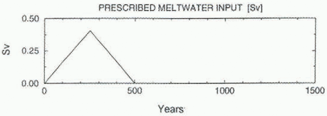
Fig. 1. Time series of prescribed meltwater input.
2. Model
The model applied here consists of the Hamburg large-scale geostrophic ocean general circulation model (Maier-Reimer and others, 1993) coupled to a two-dimensional energy-balance-typc model of the atmosphere (e.g. North and others, 1983). The model has a horizontal resolution of 3.5° on an E-grid. The ocean model has 22 levels in the vertical, with layer thicknesses ranging from 50 m at the top to 761 m at the bottom. The model has a realistic bathymetry, and a simple sea-ice model is included. The atmospheric-model component has one level, with temperature as the only prognostic variable. lèmperature changes are computed from the sum of the fluxes (radiation, air-sea heat exchange) and from horizontal transport (advection with mean climatológica] winds and diffusion). The model is forced with monthly mean climatológica! wind stress (Hel-lerman and Rosenstcin, 1983) and net freshwater fluxes from a simulation with an atmospheric general circulation model plus a flux correction term from a spin-up with restoring. The model contains a seasonal cycle. More information about the model, the spin-up and its climate can be found in Mikolajewicz and Crowley (1997).
With this set of boundary conditions three different steady states were found. (They were obtained using a number of fields from a long simulation with meltwater input into the North Atlantic as starting fields. From these fields the model was integrated in each case without external perturbation for at least 4000 years till the residual drift was negligible.) The major difference between these states is the location and strength of NADW formation. in the first mode ("strong NADW"), rather similar to the spin-up with restoring boundary condition for salinity, NADW is lormed both in the Greenland/Norwegian Sea and in the Labrador Sea. in the second mode ("reduced NADW") with weaker NADW formation, Labrador Sea convection is suppressed, and in the third mode NADW is missing completely ("no NADW"). The first two modes have outflow rates of NADW to the Southern Ocean (at 30° S)of about 12 and 10 Sv; the Atlantic northward heat transports (at 30° N) of the three modes are 0.9, 0.8 and 0.1 PW (for more information see Mikolajewicz and Crowley, 1997).
3. Experiments
In order to test the cllcct of meltwater input from the Antarctic ice sheet, two sets of sensitivity experiments were carried out. in the first set of experiments, an idealized meltwater spike of 500 years duration with a maximum input rate of 0.4 Sv in year 250 (see Fig. 1) was released in a point source at the coast of the Ross Sea. Three experiments were carried out, each starting from the model's different

Fig. 2. Time series of experiments with meltwater input on the Ross Sea coast. The time history Iff The input is shown in Figure 1. The data have been filtered with a 5 year running mean prior to plotting, (a) Atmosphere-ocean heat, exchange in the Southern Ocean (south of 30° S); negative values indicate ocean heat loss, (b) As (a), but for the North Atlantic (north of 30°) and Arctic Ocean, (c) As (a), but for the North Purifie (north of 30°N). (d) Net outflowfrom the Atlantic below 1400 m depth at 30° S. Negative values indicate deep inflow from the Southern Ocean (corresponds to value of overturning stream junction al M00 m depth at 30° S in Figure 4).
steady states with strong, reduced and no NADW formation. After the end of the meltwater input, the integration was continued for another 1000 years without further external perturbation, to give an estimate of the further development of the system. Time series of integral parameters characterizing the state of the climate system in these experiments are shown in Figure 2.
In all three experiments, the surface freshening in the Ross Sea, resulting immediately from the prescribed meltwater input, creates a stable stratification, suppressing deep convection. Through advection with the ACC, the fresh anomaly is spread over the entire Southern Ocean, also reducing deep conv ection in the Weddell Sea. The stable stratification Strongly reduces the mixing of the wintertime cold and fresh surface layer with the warmer and saltier water masses below, resulting in a strongly reduced heat loss of the ocean, enhanced sea-ice cover and surface cooling. This effect is obvious in the time series shown in Figure 2 and in the changes in air temperature shown in figure 3a.
The “no NADW” mode has a higher level of deep convection and heal loss in the Southern Ocean than the modes with NADW formation, so this mode does nol reach quite as low oceanic heat loss in the Southern Ocean. At the time of maximum rale of meltwater input (around year 250 of the experiment), deep convection is essentially restricted to the southern Indian Ocean. Convection in the Weddell Sea is restricted to intermediate depths. As a result of this heavy reduction in AABW formation, the deep ocean in the run starting from the “no NADW” mode is almost stagnant. Consistently, deep inflow of AABW into both the Atlantic and Pacific is reduced heavily (from 4 to less than 1 Sv in the Atlantic (see fig. 4a and b), and from about 8 to 3 Sv in the deep Pacific). in the olher runs, inflow of AABW into the Atlantic and Pacific is reduced as well, but the reduced formation of AABW is compensated to some extent by slightly enhanced NADW formation and outflow to the Southern Ocean. in the “no NADW” run, the stable surface stratification in the Norwegian Sea is eroded by enhanced northward flow along the European coast, and shallow convection starts, leading to a shallow overturning cell of more than 2 Sv (see fig. 4b). A similar intensification of shallow convection and shallow overturning cell can also be seen in the North Pacific with a strength of approximately 3 Sv (not shown). These overturning cells are accompanied by enhanced northward heat transport in both oceans (see Fig. 2), leading to a surface warming throughout the entire Northern Hemisphere (see fig. 3a). When the prescribed source of meltwater is reduced again, the vertical stratification in the Southern Ocean becomes less stable, and deep convection eventually recovers, especially in the Weddell Sea. Consistently, inflow of AABW into both the Atlantic (see fig. 4c) and the Pacific increases again, starting at mid-depth, but rapidly intensifying and deepening. The cooling in the Southern Hemisphere becomes restricted to the Pacific sector of the Southern Ocean (see fig. 3b).
After the meltwater input is halted in year 500, convection in the Southern Ocean intensifies strongly. in both runs initiated from the two modes with NADW, there is some overshooting, before all integral time series slowly return to the values they had at the beginning of the experiment. in the run starting from a “no NADW” state, the shallow convection in the North Atlantic and North Pacific intensifies and deepens, leading to a further enhancement and deepening of the overturning cells and an intensification of

Fig. 3. Changes in surface air temperature mm/tared to the initial stale for the “no NADW” run with meltwater input into the Ross Sea. Shown are averages overyears 276-300 (a), 476-500 (b) and the final stale (average over years 1476-1500) (c). Isolines are plotted for 16°, -8°, -4°, -2°, -1°, 0°, 1°, 2°, 4°, 8° and 16°C. Shading indicates colder temperatures compared to the initial state of the “no NADW” rim.
the northward heat transport (see Fig. 2) with further surface warming (see Fig. 3). Whereas the overturning cell in the North Pacific after reaching maximum amplitude of 4Sv with a heat loss from the ocean to the atmosphere of 0.36 PW (north of 30° N) in year 500, weakens again and the circulation approaches the normal state, the deepening and strengthening of the North Atlantic overturning cell continues. The Atlantic overturning circulation converges towards the state of the mode with “reduced NADW” (see fig. 4d). Thus it is clear that a mode switch has taken place. This transition is accompanied by passing through an area in state space characterized by a Hopf bifurcation ( in the form of strong interdecadal oscillations between years 400 and 500, visible, for example, in the North Atlantic atmosphere-ocean heat release; see fig. 2b). in this case, the perturbation in the Southern Ocean was large enough to trigger a mode switch of the Atlantic thermohaline circulation from the “no NADW” mode to the “reduced NADW” mode. The initial shallow overturning cell transported a sufficient amount of salty subtropical waters to the regions of convection to enhance and deepen convection in the Norwegian Sea, thus leading to a strengthening of the overturning cell.
In order to test whether the mode switch from the mode with “no NADW” to a mode with NADW was only an artefact of a marginal stability of the initial mode, the cxperi-ment starting from the “no NADW” mode was repeated
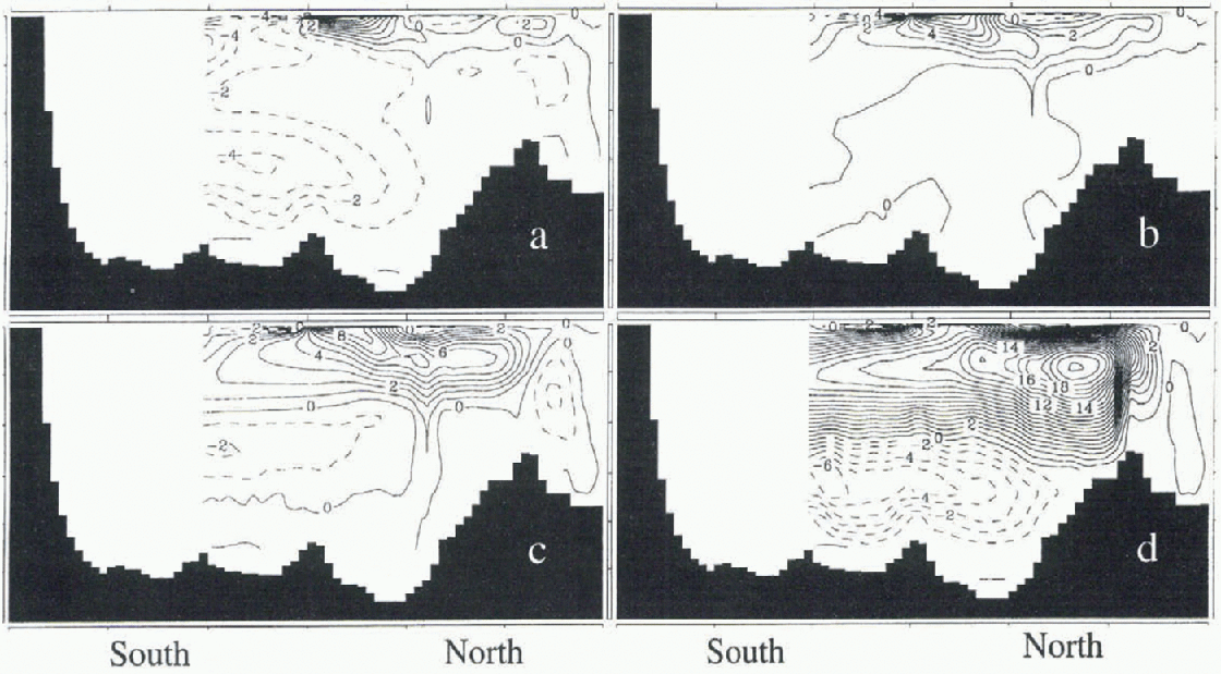
Fig. 4. Zonally integrated mass-transport streamfunction of the Atlantic for selected time intervals of the “no NADW” experiment with meltwater input into the Ross Sea. The panels show the initial state (a), and averages over the years 276-300 (b), 476-500 (c) and 1476-1500 (sd). Positive values indicate a clockwise rotation. The contour interval is 1 Sv. Isolines with negative values are dashed. The lack of solid meridional boundaries makes this quantity meaningless south of 30° S in the Atlantic
with halved input rates. The response (not shown) was still a temporary reduction of AARW formation, but the reduction reached a maximum amplitude of only 0.4 PW in Southern Ocean heat loss (compared to almost 1 PW in the standard case) around year 300 and was not sufficient to completely suppress AABW formation and initiate the mode switch.
In the other set of experiments, the meltwater was released in the Weddell Sea. Time history of the input rates was chosen to be identical to the previous case shown in Figure I. Again, three experiments were performed, initialized with the three different steady-state fields. Characteristic time series from these experiments are shown in Figure 5. Aga in the meltwater input leads to a suppression of deep convection close to the location of input, in this case the Weddell Sea. As the Weddell Sea contributes a larger fraction of the model's AABW formation, the signal in the integral quantities like heat release of the Southern Ocean is significantly stronger and relatively fast, as the meltwater is injected very close to the model's major formation site of AABW. Already in year 75 deep convection is completely suppressed in the Weddell Sea. The fresh anomaly spreads all over the Southern Ocean, till deep convection in the Southern Hemisphere is restricted to a small area off the coast of Antarctica, south of Australia. Again, the suppression of AABW formation leads to enhanced (and deeper) outflow of NADW with stronger northward heat transport. in the “no NADW” mode a shallow overturning cell develops in the Atlantic, and the system performs a transition to modes with NADW (around year 300). During the reduction of the meltwater input, the stratification in the Weddell Sea becomes less stable, and convection slowly starts to deepen. Strong deep convection starts again in year 450, rapidly increasing in strength, leading to a substantial overshoot due to the accumulated pool of warm salty waters in the deep Southern Ocean. This newly formed dense AABW penetrates rapidly northward, weakening the overturning cell of NADW. in the experiment started from the mode with strongest NADW formation, this temporary weakening of the overturning is sufficient to shut off convection in the Labrador Sea around year 600 (showing up as a sudden drop in North Atlantic heat loss in figure 5b) and to trigger the transition towards the “reduced NADW” mode. At the end of this set of experiments, all three simulations end up in the “reduced NADW” mode. in all cases, the reduction of the deep ventilation of the Pacific leads to the development of a shallow overturning cell of approximately 3 Sv in the North Pacific with increasing northward heat transport in the North Pacific (see fig. 5c). As soon as the North Pacific heat loss exceeds 0.35-0.4 Sv, it increases rapidly in strength as strong overturning cells develop (up to 14Sv, reaching down to 1900 m, in year 400 in the “no NADW” run). The other experiments show a similar, but somewhat weaker and delayed, behaviour. After this, the overturning cells and the North Pacific heat loss slowly weaken. When the heat loss reaches avalué of about 0.4 PWand the cells reach strengths of 3-4 Sv, they become unstable and collapse suddenly. in the time series of North Pacific heat exchange (see fig. 5c) this shows up as sudden reduction in heat release from about 0.4 to about 0.2 PW between years 730 ("strong NADW” run) and 1030 ("no NADW” run).
4. Summary and Conclusion
Meltwater input from the Antarctic ice sheet tends to reduce AABW formation and, with some delay, to enhance the overturning cells in the North Atlantic and North PacifiC. The associated changes in oceanic heat transport lead to a warming in the Northern and a cooling in the Southern Hemisphere. The model reacts more sensitively to meltwater input into the Weddell Sea than into the Ross Sea. Given a perturbation above a threshold value, which depends on the location of the input, it is possible to initiate switches between different steady states of the ocean thermohaline circulation with meltwater input from the Southern Ocean, thus transforming a short-term forcing signal into a long-term climate signal. It must be expected that
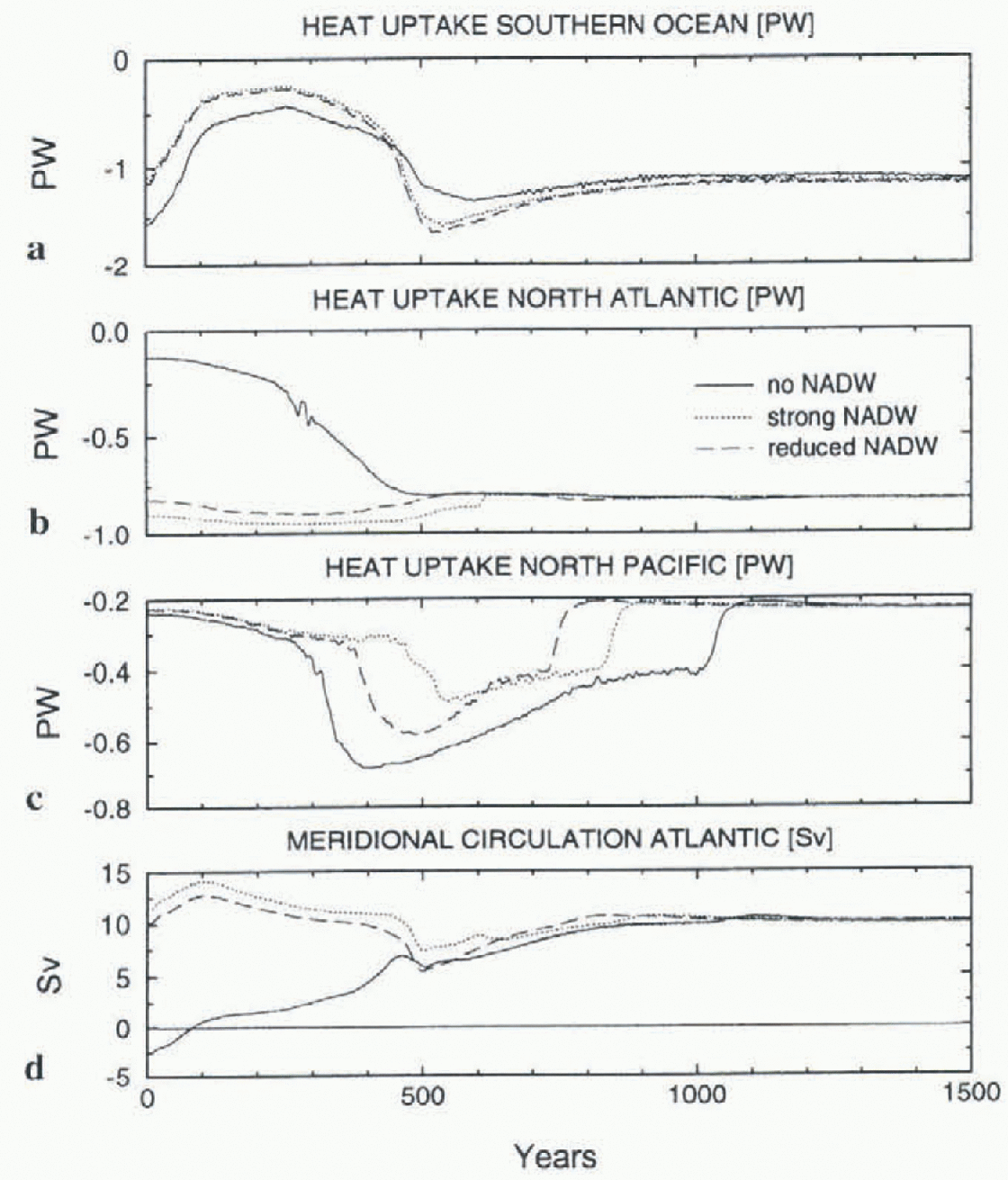
Fig. 5. Time series of experiments with meltwater input at the coast of the Weddell Sea. The time history of the input is shown in Figure 1. The data have beenfiltered with a Jijear running mean prior to plotting, (a) Atmosphere-ocean heal exchange in the Southern Ocean (south of 30° S); negative values indicate ocean heal loss, (b) As (a), but for the North Atlantic (north of 30° N) and Arctic Ocean, (c) As (a), but for the North Pacific (north of 30° N). (d) Net outflow from the Atlantic below 1400 m depth at 30° S in Sv. Negative values indicate deep inflowfrom the Southern Ocean.
very large rates of meltwater input supplied for a long time will suppress the formation of both AABW and NADW, as the surface freshening is spread all over the oceans, potentially leading to a decoupling of the deep ocean from surface levels. in this case, turbulent vertical diffusion (e.g. produced by internal tides) would need to reduce the vertical stability to enable new deep convection.
The amounts of freshwater input from Antarctica (cither direct meltwater or iceberg discharge with subsequent melting, as long as most of the melting occurs in the Southern Ocean) required in the present study to initiate a switch between different modes of the North Atlantic thermohaline circulation have similar magnitudes to the long-term average rates of global mean sea-level change during deglaciation and thus are not unreasonable.
It is likely that the numbers obtained in this study have large error bars, but the order of magnitude is probably correct. Due to the absolute size of the errors, the computation of a hysteresis diagram would not be very meaningful. It is obvious that more work is required. in particular, simulations with a fully coupled ocean-atmosphere general circulation model to account for all feedback processes would be desirable.
To unravel the history of changes in NADW formation and their causes, it is not sufficient to study only the history of meltwater/glacier discharge around the North AtlantiC. Some of the changes in NADW production may have been caused by events in the Southern Ocean.
Acknowledgements
The paper has benefited from discussions with E. Bard and E. Maier-Reimer and from the comments of the reviewers. The figures were prepared by S. Schultz. This work was in part funded by the German WOCE program of the BMBE


