


Introduction
Sea ice in the Arctic regions is affected by extensive melting during summer. The ice cover is reduced from about 15 × 106 km2 in March to about 7 × 10⁶ km2 at the end of summer (Reference Parkinson, Comiso, Zwally, Cavalieri, Gloersen and CampbellParkinson and others, 1987). The reduction of ice coverage and total ice volume takes place through a combination of surface, bottom and lateral melt. Reference Maykut and PerovichMaykut and Perovich (1987) estimated that the fraction of surface melting accounts for up to 50% of the whole melted volume, with the other two processes contributing 25% each. The extent of surface melt exhibits a strong meridional gradient in the Arctic Ocean. Russian drift-station data show an increase of surface ablation from <0.2 m ice a−1 in the central Arctic to up to 1.0 m a−1 over the Siberian shelf seas (Reference RomanovRomanov, 1993).
The extent of surficial melt depends on the total surface ablation, the permeability of the underlying ice layers and the forces driving vertical and horizontal advection of meltwater. Of these processes the former has been studied in detail during numerous field campaigns (Reference UntersteinerUntersteiner, 1961; Reference HansonHanson, 1965; Reference LanglebenLangleben, 1969; Reference Makshtas and PodgornyMakshtas and Podgorny, 1996), but the latter two have received little or no attention. The appearance and persistence of surface melt puddles, for example, depends strongly on the amount of meltwater percolating downwards (controlled by permeability) and the horizontal exchange between the low-albedo puddle and the surrounding white ice. The permeability and meltwater fluxes control the temporal evolution of ice albedo during the course of the melt season (Reference Maykut and UntersteinerMaykut, 1986; Reference Morassutti and LeDrewMorassutti and LeDrew, 1995). A typical sequence consists of an initial retainment of meltwater in a shallow layer of vast expanse at the ice surface and within the remaining snow layer (lowering of albedo), followed by drainage and lateral shrinkage of these extended melt puddles (increase in albedo (Reference Fetterer and UntersteinerFetterer and Untersteiner, 1998; Reference Eicken, Krouse, Kadko and PerovichEicken and others, 2002)). The permeability also affects the transport of particulate and dissolved matter through the ice, which influences nutrient supply to biological sea-ice communities (Reference CotaCota and others, 1987; Reference Hudier and IngramHudier and Ingram, 1994).
While the importance of permeability has been identified in studies of oil pollution (Reference Wolfe and HoultWolfe and Hoult, 1974; Reference MartinMartin, 1979) and salt fluxes in new ice (Reference Cox and WeeksCox and Weeks, 1975; Reference Eide and MartinEide and Martin, 1975; Reference Ono and KasaiOno and Kasai, 1985; Reference Wettlaufer, Worster and HuppertWettlaufer and others, 1997), actual measurements of intrinsic sea-ice permeability are only available from Reference Kasai and OnoKasai and Ono (1984) and Reference Saeki, Takeuchi, Suenaga, Murthy, Connor and BrebbiaSaeki and others (1986). Both studied artificial young ice grown in a small tank, thus not taking into account the time evolution of secondary pore space, which is crucial in determining the permeability of thicker ice. Furthermore the strong temperature gradients in the thin ice lead to a strong vertical heterogeneity of permeability and induce phase changes with brine percolating through the ice (Reference Kasai and OnoKasai and Ono, 1984). Reference Golden, Ackley and LytleGolden and others (1998) found that young sea ice displays the same critical behavior characteristic of a percolation transition, as it is known, for compressed powders of large polymer particles. However, the analogy in pore structure is restricted to the brine layers of columnar sea ice, ignoring the development of drainage structures during aging.
While in situ measurements of permeability are a standard technique in hydrogeology (Reference Freeze and CherryFreeze and Cherry, 1979), very little has been done to apply this approach to sea ice. The only study of which we are aware is the work by Reference Milne, Herlinveaux and WiltonMilne and others (1977) who recorded the flooding of blind holes drilled at three sites on multi-year ice floes. They tested the applicability of the Darcy formula, but did not derive actual permeabilities. Our approach was to apply a single-hole bail test, determining the non-stationary readjustment of the water/brine level in the borehole with a high spatial and temporal resolution. Apart from assessing the permeability, it will be shown that the transition point between turbulent and laminar inflow can be utilized to derive a characteristic pore scale controlling the macroscopic permeability.
Tracer studies of meltwater fluxes are a standard technique in glacier hydraulics (Reference Behrens, Oerter and ReinwarthBehrens and others, 1983; Reference GasparGaspar, 1987; Reference KässKäss, 1992). In sea-ice research, dyes have been employed to visualize small-scale exchange processes (Reference BenningtonBennington, 1967; Reference Eide and MartinEide and Martin, 1975). Experiments on a scale of square meters directed towards quantification of meltwater and brine fluxes have not been carried out to a large extent, however. The exchange of nutrients, in particular in the bottom ice layers, has been quantified in several ice biological studies (Reference CotaCota and others, 1987; Reference Arrigo, Kremer and SullivanArrigo and others, 1993; Reference Hudier and IngramHudier and Ingram, 1994). In a pilot study, Reference WeissenbergerWeissenberger (1994) employed a photometric technique to determine lateral brine and meltwater migration in Arctic sea ice. The study demonstrated the need for refined sampling techniques and increased sensitivity. In this study, experiments devoted to the quantification of lateral meltwater fluxes on summer Arctic sea ice have been carried out utilizing fluorescent tracers and newly developed sampling techniques.
The overall aim of this contribution is to provide permeability data of natural summer Arctic sea ice, obtained during two ship expeditions in 1995 and 1996, to estimate the constraints on vertical brine and meltwater percolation through the ice matrix. Furthermore a first tracer-based dataset of lateral surface meltwater fluxes is presented to assess the larger-scale permeability and driving forces. This may also allow for a critical reappraisal of the assumption underlying previous studies of Arctic ice growth and ablation, namely that the flux of meltwater andenergy through sea ice canbe considered as a one-dimensional problem, ignoring lateral advection and exchange, and is not controlled by the hydraulic permeability of the ice cover. The latter problem has been addressed in more detail in a follow-up study as part of the Surface Heat Budget of the Arctic Ocean (SHEBA) study (Reference Eicken, Krouse, Kadko and PerovichEicken and others, 2002).
Hydrological Background
The migration of fluids through a porous medium depends on its permeability. The permeability of a porous medium is defined in the empirical law of Darcy, that describes the linear relationship between discharge and driving force, when a fluid is forced through the pores of a porous medium:
with specific discharge u (m s−1), imposed effective pressure gradient ∇p (N m−3), permeability k (m2) and dynamic viscosity η (kg m−1 s−1). The permeability is a property of the porous medium which allows advection of fluid through the connected pathways along their geometry. For the simple geometry of a tube the permeability is proportional to the cross-section area of the tube. The specific discharge is the volumetric flux through a vertically oriented cross-section area including solid and void faces. In the case of exclusively gravitational forces, the imposed pressure gradient can be expressed by the hydraulic gradient ρgΔH/ΔL in the direction of the main fluid flow, with density ρ (kg m−3), gravitational acceleration g (m s−2), and water-level difference ΔH (m) between two selected observation points and their lateral distance ΔL (m). The applicability of Darcy’s law is limited to the case of laminar flow. The limit is usually identified with the aid of the dimensionless Reynolds number Re, expressing the ratio of inertial to viscous forces:
with a characteristic flow velocity U (m s−1), the dynamic viscosity η (kg m−1 s−1) and a characteristic pore dimension r (m) such as the mean pore or tube radius. In a tube, the critical Reynolds number for the transition between laminar and turbulent flow has been measured to Rec = 2300 (Reference SchlichtingSchlichting, 1982). For porous media with a complex pore structure, the transition is gradual and occurs for critical Reynolds numbers of 1–10 (Reference BearBear, 1972). In the case of turbulence and even for more dominant inertial forces, the specific discharge is no longer a linear function of the imposed pressure gradient, but decreases relative to laminar flow. Concepts for the description of turbulent flow through porous media are reviewed in Reference MarsilyMarsily (1986).
The pore space of sea ice consists of primary and secondary pores. Primary pores are formed as brine pockets at the ice–water interface during freezing. It is a fine network of mainly layered structure with characteristic pore sizes of 0.1 mm or less. During ice aging, and due to brine drainage, a fraction of the primary pore space is transformed to a set of vertically oriented tubular drainage structures attended by smaller, radially orientated tributary tubes (Reference Weeks, Ackley and UntersteinerWeeks and Ackley, 1986). These secondary pores, being 0.1 to a few mm in size, are therefore much larger and could determine the permeability of the whole pore space. In the limit of only one vertically oriented tube-like pore within an ice cylinder of radius R, the pore radius r max and the permeability k of the ice cylinder are related by
Assuming laminar flow, the mean velocity can be expressed by Hagen–Poiseuille’s law. The mean velocity is set to equal the specific discharge derived from Darcy’s law multiplied by the ratio of cross-sectional areas between the ice cylinder and the pore tube. Equation (3) is determined by separating the pore radius. In bail tests (discussed below) r max is used as a rough estimate of an upper limit of pore size. For these calculations, R is the radius of the ice cylinder beneath the blind holes.
During summer, brine and meltwater motion in the sea-ice system can be driven by external imposed pressure gradients or by internal density variations. At free meltwater surfaces, airflow induces a lateral pressure gradient. At the bottom and the side faces of ice floes, the internal pore system is in contact with the open water and therefore sensitive to ocean currents. Gravitational forces act on meltwater that is formed on ice surfaces above sea level. Any rise or depression of an ice floe, assuming a new isostatic equilibrium, can also induce an imposed hydraulic head.
Area of Investigation
The hydrological field experiments were carried out during two expeditions in successive summer seasons in the northern Laptev Sea and central Arctic (Fig. 1). During the joint Russian–German ARCTIC 95 expedition of RV Polarstern in July–September 1995, almost the entire study period was characterized by typical summer conditions of melting first-year ice with melt-puddle coverage of 30–50%. During the expedition ARCTIC 96 with the Swedish icebreaker Oden in August and September 1996, the experimental sites were located more to the north. Different ice conditions in 1996 led to greatly reduced surface ablation, with melt-puddle coverage <1% and a substantial snow cover remaining throughout the summer (Reference Haas and EickenHaas and Eicken, 2001). Most of the ice sampled was second- or multi-year; with the aid of a buoy deployed in 1995, a first-year ice field studied during ARCTIC 95 was resampled in 1996.

Fig. 1. Map of the site locations during the expeditions in 1995 and 1996. The position of a buoy deployed in 1995 and resampled in 1996 is also indicated.
In Situ Permeability Measurements
Method
The permeability has been derived from bail tests on blind holes, drilled at different spots within the sea-ice cover. In a bail test, the adjustment of the water-level horizon to equilibrium is analyzed. Such bail tests are widely used in hydrogeology (Reference DullienDullien, 1979; Reference Freeze and CherryFreeze and Cherry, 1979) and have been adapted for sea-ice conditions. Figure 2a shows a sketch of the experimental set-up. The blind holes with a fixed diameter of 91 mm and variable length were sealed lengthwise by an aluminum tube, which effectively sealed the perimeter of the core hole. The water level was measured with an ultrasonic sensor mounted on top of the tube with a resolution of ±0.5 mm and a maximum sampling rate of 20 Hz. Prior to every measurement, water was removed with a valve bail to induce flow into the sealed hole. At the end of each measurement, the total ice thickness and the fraction of ice under the blind hole were measured by drilling.

Fig. 2. (a) Experimental set-up of an in situ bail test. (b) A time series of the hydraulic head recorded within the borehole. The measurements are represented by open circles; the dashed line is an exponential fit to the data in the laminar branch of the curve.
Figure 2b displays a typical time series of the hydraulic head h(t). The hydraulic head describes the difference in height between the actual water-level horizon and the equilibrium sea-water level. In general, the hydraulic head decreases in a step-like fashion followed by an exponential decay. Figures 2b and 6 show h(t) curves with a single transition point in the range 0.05–0.10 m. This behavior identifies two different flow regimes during one measurement. At high hydraulic heads when the inflow into the blind hole starts and the local flow velocities are at their maximum, the fluid migration through the pore space is dominated by inertial forces or could even be turbulent. During the ensuing inflow, the hydraulic head and the specific discharge are continuously decreasing. The pronounced discontinuities in the curves suggest transitions between turbulent and laminar flow. In the laminar flow regime, the hydraulic head shows an exponential decay, gradually subsiding to zero. Assuming Darcy’s law (Equation (1)) for the laminar branch requires that the specific discharge (= dh/dt) is proportional to the driving force, here expressed by the hydraulic head h(t). Assuming furthermore exclusively vertically oriented pores such that inflow only affects the ice volume directly underneath the borehole cross-section, the recovery curve is given as
with hydraulic head h(t) (m), permeability k exp (m2) and ice thickness L (m) underneath the borehole. The data are well described by an exponential function. The exponent of the fitted function would thus provide a value for a vertical permeability under the assumption that sea ice is laterally impermeable. Laboratory experiments indicate, however, that the ice has a non-zero lateral permeability (Reference FreitagFreitag, 1999). On average, permeability is one order of magnitude lower in the horizontal than in the vertical direction. To take the lateral permeability into account, we derived a correction function from numerical simulations. The threedimensional simulations were carried out using the software Modflow, which is based on a finite-differences approach of fluid motion in porous media (Reference KinzelbachKinzelbach, 1995). Figure 3a–c illustrate the modeled shift of the equipotential pressure lines by varying the ratio k/k v of lateral to vertical permeability. The regime of inflow under the blind hole becomes wider with increasing k l /k v. For all ratios the exponential form of the simulated recovery curves is preserved. The simulation runs were done with k l /k v → 0 (only vertically permeable), k l /k v = 0.01, 0.1 and 1 (isotropic medium). The permeability kexp derived from the recovery curve of a measurement based on Equation (4) corresponds to the case of k l/k v = 0 and has to be converted into the more realistic case of k l/k v = 0.1 (Reference FreitagFreitag, 1999). To this end, a correction factor γ is introduced. γ is defined as the ratio of the discharge through a laterally permeable medium and the discharge through a laterally impermeable medium, assuming equal values for vertical permeability, imposed hydraulic heads and geometrical dimensions:
γ is independent of the absolute value of vertical permeability and imposed hydraulic head, but depends on geometric parameters. Following Darcy’s law (Equation (1)) in the case of exclusive vertical permeability, the discharge is inversely proportional to the ice thickness L underneath the blind hole. As shown in Figure 4, this negative correlation breaks down in the case of additional lateral permeability, which is expected because increasing L leads to increasing lateral fluxes. Except near the ice surface and bottom, the total discharge remains constant and tends to increase towards both boundaries. Different total ice thicknesses do not change the discharge level, but separate the boundary effects. However, it is evident that for increasing ratio k l/k v the discharge increases as well. From the model results it is established that γ depends linearly on the ice thickness under the blind hole with rising slopes for increasing ratios k l/k v (Fig. 5). The linearity is limited to blind holes in the interior of the ice column, at least 20 cm away from either boundary, which is fulfilled for 95% of the drilled holes. Under these restrictions γ(L) can expressed by

and the ice thickness L (m). Overall, the vertical permeability k v of sea ice is derived from measurements using Equation (4) for the laminar branch of h(t) to estimate k exp followed by a correction with γ 0.1(L) that yields
The expanded measurements of inflow not only in the laminar flow regime but also for the inertial and turbulent flow regimes provide further information about the pore structure of sea ice. For a homogeneous porous medium with a highly tortuous and connected pore structure, the transition between different flow regimes is very weak and not detectable in a h(t) curve. In contrast, the h(t) curves of sea ice show sharp transitions. Most probably the transitions take place in the large tubes of the secondary pores. This implies that the flow through the few such large pores dominates the whole discharge, since otherwise the transition signal would not be apparent in the h(t) curves. It seems that the vertical permeability of sea ice is controlled by secondary pores, with the consequence that fluid migration is mainly restricted to such pores at least during the summer period. To confirm the explanation of the discontinuities in the h(t) curves, we estimate the radius of a vertically oriented tube assuming that the hydraulic head h crit at the discontinuity corresponds to the critical value for the transition to turbulent flow. The flow field is described by Hagen–Poiseuille’s law. The mean velocity at the transition can be expressed by the critical Reynolds number. Then the tube radius r is given as


Fig. 3. Model calculations of the pressure field during a bail test for three different ratios between lateral permeability k l and vertical permeability k v. In a vertical cross-section the initial isobars are plotted for constant intervals. (a) The simulation with laterally impermeable ice; (b) the case for a ratio of k l/k v = 0.1; and (c) the isotropic case with k l = k v .

Fig. 4. Relationship between discharge and ice thickness L underneath the borehole in a simulated bail-test geometry. The model runs are performed in ice with k l/k v = 1(isotropic), 0.1, 0.01 and 0 (laterally impermeable). The hydraulic head is kept constant. The total ice thickness is 1, 2 and 4 m.

Fig. 5. Relationship between the derived correction factor γ and ice thickness L underneath the borehole. γ depends linearly on L with rising slopes for increasing k l/k v ratio which reflects the enhanced inflow due to lateral permeability.
The position of the discontinuity in the measured h(t)curve determines the hydraulic head h crit. If multiple discontinuities occur, then that corresponding to the lowest hydraulic head is chosen for h crit. The phenomenon of multiple transitions is the result of a temporary increase of the Reynolds number after a transition from turbulent to laminar flow due to large velocities in the case of laminar flow. In the vicinity of Recrit and large hydraulic heads, Re can shift several times from values above and below Recrit. Here, a critical Reynolds number of 2300 is assumed based on measurements in undisturbed pipe flow (Reference SchlichtingSchlichting, 1982).
The permeability is very sensitive to changes in pore space. A change of one order of magnitude in the radii of a vertical bundle of tubes would change the permeability by 4 orders of magnitude (Equation (3)). However, the pore space of sea ice depends on temperature and brine salinity. For example, drainage networks formed during the melt period significantly change the character of the pore space. Bailtests take the characteristic sea-ice features into account and avoid pore-space changes in so far as fluid with slightly different temperature and salinity is only flowing through pores during the measurement itself. Repeated measurements at the same borehole show the permeability changes caused by the measurement itself (Fig. 6). The rate of increase in water level grew with every measurement. The derived permeability increases by roughly 7% per measurement cycle. This increase is caused by the inflow of warm, more saline water. Such effects are monitored for each location, and consequently the extrapolated permeabilities for the limiting case of unchanged pores have been reduced by 2–10% depending on the measured widening effect.
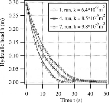
Fig. 6. Time series of the hydraulic head measured repeatedly at the same blind hole.
The bail tests sample an ice volume on a scale of cubic meters and are thus more affected by heterogeneities than are laboratory measurements. Nevertheless, the effective pore-channel values derived from the transition points refer only to the ice volume close to the blind hole, where the inflow velocity has its maximum. Uncertainties in the derived permeabilities mostly originate from the specification of the ratio between lateral and vertical permeability. The geometric mean of permeability decreases by approximately a factor of 0.3 when the ratio k l/k v = 0.1 is replaced by 1 (case of isotropy). In comparison, uncertainties due to the measurement process and the exponential fit (6%) are negligible. In principle, the bail-test method is limited to the ice below freeboard and yields integrated values of vertical permeabilities.
Results
At 24 stations 122 measurements were carried out in 46 different boreholes. The hole depths ranged between 0.6 and 1.70 m in ice of total thickness 0.8–5.25 m. The lower branches of the recovery curves are very well described by exponential fits, with a weak systematic deviation due to transitions to laminar flow. The total error of the exponent is estimated as 6% because of the uncertainty in identifying the upper limit of the fit interval, which represents the limit of the fully developed laminar flow regime. At 29 boreholes (63%) the recovery curves indicate a clear transition between turbulent and laminar inflow.
The vertical permeabilities of summer Arctic sea ice derived from the recovery curves are in the range 10−11–10−7 m2, with geometrical means of 8 × 10⁻¹⁰ m2 (1995) and 4 × 10⁻¹⁰ m2 (1996) (Fig.7). The vertical permeabilities represent integral values of the lower entire section of the ice cover. Mean and modal permeabilities differ by one order of magnitude between measurements in 1995 and 1996. These differences are explained by the differences in ice age and, in particular, the highly contrasting thermal regimes with a climatological decrease in ablation to the north (Reference RomanovRomanov, 1993) and an unusually cold melt season in 1996 (Reference Haas and EickenHaas and Eicken, 2001). The ice permeabilities are comparable to those of sand and karst systems (Reference Freeze and CherryFreeze and Cherry, 1979). In these systems, subsurface drainage systems similar to those in sea ice are created due to the karstification process. There usually exists a continuous path made up of larger pores to which most of the flow is confined (Reference DavidDavid, 1993).

Fig. 7. (a) Frequency distributions of in situ permeabilities measured during the expedition in summer 1995 (solid line), 1996 (dotted line) and for artificial sea ice measured by Reference Saeki, Takeuchi, Suenaga, Murthy, Connor and BrebbiaSaeki and others (1986) in the laboratory (dashed line). (b) The fate of meltwater illustrated in a cross-section through an ice floe. Depending on permeability, the meltwater either percolates downwards and disappears from the ice surface (k>k crit) or is partially retained at the ice surface (k<k crit).
The hydraulic similarity of sea ice to karst systems suggests that the “critical path” of these pores determines the permeability of Arctic sea ice in summer.
Compared to measurements on artificial sea ice at temperatures of −5 to −20°C by Reference Saeki, Takeuchi, Suenaga, Murthy, Connor and BrebbiaSaeki and others (1986), permeabilities of summer Arctic sea ice are at least two to three orders of magnitude larger. Such comparatively high permeability is explained by the evolution and widening of the secondary pore-channel system in Arctic sea ice, mostly as a result of brine drainage and internal melting processes. The clear transition from turbulent to laminar flow in the borehole experiments suggests that the permeability of ice is controlled by individual large tubes or channels. For those sets of measurements exhibiting a distinct transition point in the recovery curve, a tube radius has been calculated based on Equation (7) (Fig. 8). The tube radii are in the range r e = 0.5−2.5 mm and correspond to the upper limit of pore-channel sizes reported by other authors (Reference MartinMartin, 1979; Reference Wakatsuchi and SaitoWakatsuchi and Saito, 1985). However, the correlation between permeability and tube radius is not definite. Higher permeabilities do not always imply higher tube radii.
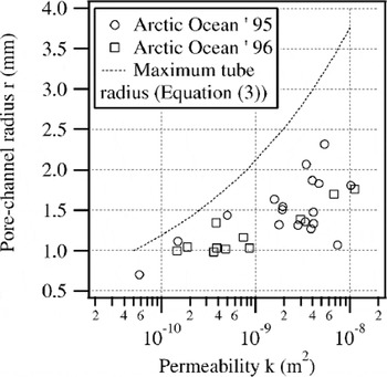
Fig. 8. Pore-channel radii derived from flow-regime transitions in the measured time series vs permeability. Data of the 1995 expedition are shown as open circles, data for 1996 as open squares. For comparison, the maximum accessible tube radius is plotted as a dotted line based on Equation (2).
Tracer Studies
Method
With the aid of non-reactive dye tracers, fluid flow through the ice can be directly recorded. In the tracer experiments, the dye has been injected into the water of boreholes or melt ponds on the ice floe, measuring the dispersion of fluid at different sample positions around the injection point. The progression of the peak in dye concentration allows an estimate of the average specific discharge. If the driving forces are known, such as the hydraulic head between two sample positions, a lateral permeability can be calculated based on Darcy’s law (Equation (1)).
The tracer has to be non-reactive in the sea ice, such that the adsorption onto the ice matrix and the photochemically induced decay is negligible during the measurement interval. For our tracer studies, the fluorescent dyes fluorescein (F) and sulforhodamine B (S) were chosen as tracers (Reference GasparGaspar, 1987; Reference KässKäss, 1992). Fluorescein with a low tendency to adsorb onto ice surfaces and a low detection limit on the order of 10−6 mg L−1 is suitable for short-term measurements with time-scales < 1 day. For long-term experiments sulforhodamine B is used, because of its insensitivity to light decay in comparison with fluorescein. However, the detection and the adsorption limit of sulforhodamine B are 2 orders of magnitude higher than those of fluorescein. Reference KässKäss (1992) gives an overview of further physical characteristics.
The dye concentration was determined by fluorometric analysis at excitation wavelengths of 491 nm (F), 565 nm (S), corresponding to the emission maximum at 512 nm (F), 590 nm (S). The intensity of the fluorescence signal depends linearly on the dye concentration over 6 (F) and 4 (S) orders of magnitude. The different excitation and emission wavelengths of fluorescein and sulforhodamine B allowed simultaneous use of both tracers. The fluorometric analysis is specific for a substance and insensitive to pollution. Because of the temperature dependence, all fluorescence measurements were carried out at the same temperature of 10°C in the laboratory on board the research vessel.
An experimental site consisted of an array of blind holes (ϕ = 0.05 m, drilled to >0.5 m below sea level) for water sampling during the measurements (Figs 9 and 10). Drilling or ice coring immediately prior to sampling or after dye injection is problematic for small-scale studies, since the removal of a substantial ice volume induces non-negligible fluid flow that may thwart the actual measurement. Therefore the injection of dyes into the center hole or melt pond was delayed for 30 min until the water levels in the holes had reached equilibrium. About 200 mg of dye dissolved in 50 mL meltwater was mixed with the water of the center hole. After injection, 5–10 mL of water was drawn every 6 hours from the sampling locations. Dye concentrations were determined on board the research vessel with a HITACHI F2000 fluorometer directly after sampling.

Fig. 9. Tracer site R11219/220 in deformed ice with concentration profiles along four transects (T1, T2, T3, T4). The graphs show the profiles 3 hours (solid circles) and 16 hours (open circles) after dye injection. Gray areas are melt ponds.

Fig. 10. Tracer site R11220/221 in deformed ice with concentration profiles along three transects (T1, T2, T3). The graphs show the profiles 9.5 hours (solid circles), 16 hours (open circles) and 22 hours (crosses) after dye injection. Gray areas are melt ponds.
Unlike bail tests, tracer studies take the driving forces into account, allowing quantitative estimates of lateral specific discharge and permeability. Tracer spreading due to molecular diffusion is in the range of centimeters per day and is therefore negligible. The observed dispersion is thus caused entirely by the motion of the fluid. Heterogeneities of the permeability due to large channels, cracks or other discontinuities enlarge the dispersion. In such cases, a mean front velocity cannot be estimated (Fig. 10, transects 1 and 2). The mass balance for the migration around melt ponds can be solved if all heterogeneities are included. Because of the simple deployment of sample locations, their density can be increased, however, to take those effects into account. The largest uncertainty consists in the quantitative specification of the relevant driving forces (e.g. the momentum transfer by surface winds). Furthermore, due to the variable light conditions, the decay of fluorescein is uncertain and its term in the mass-balance equation has an error of 30%. The accuracy can be increased when both tracers, fluorescein and sulforhodamine B, are used simultaneously. In the present configuration, the tracer test method is limited to lateral flow, since the concentration values are integrated over the entire depth of the borehole.
Results
Experiments in deformed ice with a high hydraulic gradient as main driving force
In a rubble field at station R11219/220 (Fig. 9), a melt pond (as a center location) was colored by fluorescein. The water level of the pond was 0.50 m a.s.l. The mean depth at the start of the experiment was 0.15 m, decreasing to 0.10 m 16 hours later. The sample positions are located in a segment of 120° in the sloping sector of the pond vicinity. The mean depth of the holes was 0.82 ± 0.05 m, with the water level at 0.45 ± 0.06 m.
In the directions of all transects, the marked meltwater migrated into the surrounding ice (Fig. 9). The dye concentration in the pond decreased and local concentration maxima built up within the ice. After 16 hours, a concentration peak had moved into the ice by about 1 m. Assuming a two-dimensional, divergent radial flow with a pond radius of 1.0 m, the front velocity at r = 2.0 m becomes u f = 1.3 × 10⁻⁵ m s−1 (= 0.05 m h−1). With the measured hydraulic gradient of 0.5, the derived lateral permeability is k l = 1.3 × 10⁻¹² m2 using Darcy’s law in polar coordinates.
To estimate the effective ice-layer thickness through which the meltwater is flowing, the mass balance of the dye, spreading into the ice from the pond, must be solved. The mass budget has at least two terms, the term of retained dye, diluted by water inflow into the pond, and the outflow portion of dye within the pore space of ice. Due to the light sensitivity of fluorescein, a third decay term is added. For simplification and due to the lack of information about the rate changes under different light conditions, the same decay constant is assumed for the dye in the pond and within the ice matrix. Thus, the mass balance is expressed by:

with dye concentration C (mg L−1), water volume V (m3), ice porosity n and decay constant λ (s−1). The indices i and p indicate ice and pond water values, and the index o refers to the initial values. Assuming a cylindrical pond geometry and an equal division of the surrounding ice into an inflow and an outflow area in accordance with the local topography, the mass-balance equation (8a) can be written as:

with pond surface area A p (m2), depth d p (m), radius r p (m) and effective ice-layer thickness d i (m). The decay constant has been determined as λ = 3.2×10⁻⁵ s−1 by Reference FreitagFreitag (1999) for fluorescein under comparable light conditions using a laboratory sunshine simulator. The porosity of the upper ice layer is estimated as n = 0.2 based on a density measurement (ρ = 752 kg m−3). Using the concentration values measured after 16 hours (Fig. 9) and the pond parameters (r p = 1.0 m, d po = 0.15 m, d p(16 h) = 0.10 m) the mass-balance equation (8b) gives the effective ice-layer thickness d i = 0.17 m. The ice-layer thickness has the same magnitude as the pond, indicating that the meltwater flow is confined to the surface layers.
The time t d needed to discharge the initial pond volume is the quotient of that pond volume to the mean volume flux. The volume flux is given as the product of lateral discharge u = nu f multiplied by the outflow area A = πr p d p:

t d is estimated to be 53 hours. Thus, after 16 hours approximately one-third of the pond water would have been exchanged. In the same time period, a lowering of the water level in the pond by one-third was observed. The missing volume corresponds to the expected outflowing volume. Therefore it can be assumed that there was no inflow during the observation period, which is also supported by the change of the fluorescence signal. It was approximately reduced by an amount expected for the decay due to radiation. Compared to the enhanced decay in the pond area due to direct exposure, the fluorescence signal of pore water within the ice matrix remains at a higher level. Consequently, the maximum of the fluorescence signal is found within the ice and not within the pond itself (Fig. 9).
In a further experiment at a melt pond in deformed ice, the dispersion curves show a strong heterogeneity of the lateral permeabilities of the surrounding ice (Fig. 10).
Transect 3 is located in ice of low permeability with an upper limit for k of 2.3 × 10⁻¹³ m2 and a front velocity below u f = 0.020 m h−1. The highly permeable zone of transect 2 has a lower limit for k of 9.0 × 10⁻¹² m2 and u f = 0.15 m h−1. The melt flux through the ice of transect 1 amounts to a front velocity u f1 = 0.071 m h−1 at 1.50 m distance and u f2 = 0.069 m h−1 at 2.0 m derived from different time-steps. The mean lateral permeability is determined as 4.3 × 10⁻¹² m2.
Experiments in level ice under wind stress
At station R11216 the water of a melt pond in level ice was colored with fluorescein. The small pond covered an area of approximately 1 m2 and had an average depth of 0.08 m. The sample boreholes were drilled to 1 m depth. During the 9 hour experiment the wind speed was measured at intervals of 10 min at a height of 10 m. The mean velocity was u = 11.5 ± 1.6 m s−1, and the direction varied by <4°.
The marked pond water migrated into the surrounding ice, forming a plume oriented parallel to transect 1. This direction coincides with the main wind direction (Fig. 11). During the 9 hours, the maximum dye concentration moved laterally into the ice by 1.4 m, yielding a specific discharge of u = 4.3 × 10⁻⁵ m s−1. The wind stress affects the water circulation in the pond and induces a main flux down-wind. However, a short leg of the plume also extended into the ice against the main wind direction (Fig. 11).

Fig. 11. Concentration profiles along wind direction at tracer site R11216 in level ice. The graph shows the initial concentration (solid circles) and the profile 9 hours (open circles) after dye injection.
Experiments in level ice without wind stress and large-scale hydraulic gradients
At station R11247, experiments were conducted in level ice >100 m away from the ice-floe edge. Instead of a melt pond, dye was mixed into the water in a hole at the center of the sampling array. The boreholes were 0.61 and 0.69 m deep. The sampling positions were arranged crosswise around the center hole. During the measurements, the mean wind speed was 5.2 ± 0.5 m s−1 and never exceeded 6 m s−1. Ice freeboard was 0.33 m, such that wind stress most likely did not affect meltwater flow. Because of the very flat topography, it is assumed that no large-scale hydraulic head was imposed.
In all boreholes separated <0.65 m from the center hole, low concentrations of dye were detected (Fig. 12). The measured concentrations were 4 orders of magnitude lower than the initial concentrations. No directional trend is apparent from the data. The maximum concentration remained at the center points. The decrease is exponential rather than linear. In general, the concentration decreased with distance to a center hole. However, three sample positions show higher values14 hours after t = 0 s than positions closer to the center. This indicates that lateral fluid motion on the order of 0.2 m h−1 is possible, but the motion is restricted to local discontinuities (e.g. through secondary large pores or cracks).

Fig. 12. Concentration profiles at tracer site R11247 in level ice. The graph shows profiles along two transects intersecting at right angles for the initial concentration (dotted line), and the profiles 4 hours (solid circles) and 14 hours (open circles) after dye injection.
Discussion
Based on the measurements and data presented above, we can estimate the rates of vertical meltwater percolation through the ice cover. Thus, a critical permeability k crit can be determined which separates the regime of meltwater retention and pooling at the ice surface from that allowing for complete downward drainage of melt (see Fig. 7b for illustration of k crit). Based on climatological data (Reference RomanovRomanov, 1993), we have assumed a melt-season duration of 77 days with a total surface melt of 0.53 m (water equivalent, snow and ice), yielding a mean ablation rate of 6.9 mm d−1. For Darcian flow, this results in a critical permeability of k crit = 1.5 × 10⁻¹³ m2. If we allow for periods of enhanced surface melt with ablation rates higher by a factor of 10, k crit = 1.5 × 10⁻¹² m2. All measurements presented here exceed these values of k crit, suggesting that in mid- to late summer the sea-ice cover is permeable enough to completely drain the meltwater produced at the surface. This raises the question as to what allows the formation of melt ponds (in particular those with water level above the equilibrium surface) in the first place. While lateral inflow of meltwater is of importance, it would require inflow areas larger by a factor of 100–1000 than the pond area to explain these numbers for permeabilities of 10−9 m2. With ponds covering >1% of the surface area, this is an unrealistic assumption. Rather, it appears that the permeability in the upper ice layers (for which we have few or no data), and in particular during the earlier melt season, is critical in allowing surface retention of melt. This has been independently verified in a study by Reference Eicken, Krouse, Kadko and PerovichEicken and others (2002) carried out over the entire duration of a melt season in first- and multi-year ice in the North American Arctic.
Here, we can still assess to what extent the desalination and concurrent reductions in ice porosity, a key parameter in controlling permeability, contribute to a potential lowering of permeability in the upper and interior ice layers. This includes refreezing of surface water draining into the lower ice layers, which is dependent on the temperature difference between meltwater and the surrounding ice and the residence time at a given depth level. For rapid dissipation of meltwater in highly permeable ice, one would not expect to see much refreezing due to reduced heat exchange between meltwater and ice matrix. Assuming an ice thickness of 1.0 m with a mean porosity of 0.1 and a hydraulic head of 0.1 m, we obtain mean residence times within the ice of between 2 s and 5 h for the range of permeabilities measured. The time-scale for heat transfer can be roughly estimated by considering the simplified case of laminar flow in vertical tubes. For millimeter-sized tube radii the freezing of the liquid phase takes place in seconds when initial temperature differences of 2–4°C and zero-salinity meltwater are assumed. This implies that at least in the early stage of melting, when surface snow is melting above a cold ice layer, the meltwater tends to freeze at the snow–ice interface, resulting in the formation of ice or ice plugs within pores of the upper ice layers, effectively sealing the ice surface. Such layers of superimposed ice have `been observed in earlier studies (Reference CherepanovCherepanov, 1973) as well as in recent tracer and permeability experiments (Reference Eicken, Krouse, Kadko and PerovichEicken and others, 2002). Subsequently, only complete melting of such impermeable layers would allow vertical transport of meltwater. Considering the high permeabilities of the underlying ice, the boundary conditions in the upper part of the ice are particularly important in limiting vertical percolation during summer melt. The formation of superim-posed ice and other impermeable layers is controlled by the temperature evolution and the salinity of the meltwater, depending in particular on the snow depth.
Another important aspect that affects the mass and energy balance is the lateral mobility of the liquid phase in the upper ice layers. This is supported by the results of the tracer studies in the vicinity of melt ponds. Qualitatively, fluid motion covering >50 m d−1 was observed at some locations. In deformed ice and ridged areas the probability ofencountering conduits is considerablyhigherthan in level ice, resulting in linkage and meltwater exchange between ponds. The direction of lateral movement is controlled by the formation of highly permeable zones, resulting in a hydrological heterogeneity. An example of such heterogeneity is given in Figure 10, with Figure 9 showing a contrasting, homogeneous permeable floe portion. Due to the lower albedo, the water in the melt pond absorbs more radiation than the surrounding ice and warms up to temperatures above the freezing point. The heat transported by the lateral flow can be roughly calculated for the experiment at station R11219/220. Based on measurements during the cruise, the temperature difference between meltwater and ice is assumed to be dT = 0.5 K (Reference Zachek and DarovskikhZachek and Darovskikh, 1997). With a specific discharge of u = 0.06 m h−1 the lateral heat flux is calculated to be F lat = cρA dT u = 10.6 W m−2 which is approximately one-third of the net absorbed radiation in August over 1 m2 (c: specific heat capacity; A: outflow area) (Reference Maykut and UntersteinerMaykut, 1986). Such a small-scale, positive ice-albedo feedback mechanism may thus further accelerate the melting process, as studied in more detail by Reference Eicken, Krouse, Kadko and PerovichEicken and others (2002).
Conclusions
During mid- to late summer, the hydrological properties of Arctic sea ice are comparable to a geological karst system (Fig. 7). The pore space with associated permeabilities as high as 10−7 m2 acts as a potential pathway for meltwater and controls the drainage and the amount of meltwater retained at the ice surface. Tracer studies demonstrated that the water in melt ponds is in exchange with the pore water of the surrounding ice. As driving forces, the hydraulic gradients in ridged areas and wind stress have been identified. The mobility of meltwater has important consequences, outlined below.
-
I. The extent of surface melting and hence the albedo, the emissivity and the backscatter coefficient at microwave frequencies are affected by meltwater migration. The influence on albedo can act in both directions. Vertical meltwater percolation leads to an increase of albedo, because the liquid volume above freeboard is reduced. The lateral migration of meltwater in the vicinity of melt ponds reduces the albedo, with the additional lateral heat flux increasing pond cross-sectional areas. In general, such fluid motion may be part of a positive feedback mechanism. High permeabilities enhance meltwater fluxes and transport of sensible heat, thus leading to increased internal melting, which in turn increases permeability. Presently it is not fully understood, however, to what extent meltwater advection results in reduced permeabilities or the sealing of parts of the ice cover through ice formation induced by double-diffusion processes (e.g. in the case of under-ice melt ponds (Reference EickenEicken, 1994)).
-
II. Meltwater migration through sea ice is dominated by the discharge through individual large pore channels, as is indicated by the inflow measurements during the bail tests. This implies that potential freezing or thawing acts in a heterogeneous manner, resulting in a change of pore-space size distributions in sea ice. Continuous meltwater flow forms highly permeable zones through positive feedback processes and thus enhances heterogeneity. Sealing of pores through refreezing meltwater and widening of larger pores also enhances the heterogeneity in pore sizes. Therefore meltwater percolation through mid- to late-summer sea ice should be treated as a fairly heterogeneous migration, even leaving some parts of the ice cover unaffected by meltwater flow. This is also indicated by the scale dependency of the permeability. The permeability tends to values one to two orders of magnitude higher when the scale is shifted from decimeters in the laboratory to meters in the field (Fig. 7).
-
III. Interannual variability. The two datasets obtained in 1995 and 1996 represent two extreme cases of summer melt, with high melt rates and rapid ice retreat in 1995 and little or no surface melt in 1996 (see also Reference Haas and EickenHaas and Eicken, 2001). It is remarkable that despite these contrasts, permeabilities in the middle and lower ice layers only varied by a factor of two between these two years and were high enough in all cases to allow for vertical percolation and complete dissipation of surface meltwater. Hence, we conclude that the differences between the two years are mostly a result of differences in surface melt and refreezing processes and their impact on the permeability of the upper ice layers.
Acknowledgements
Financial support from the German Ministry of Research (BMBF) and the U.S. National Science Foundation (grant OPP-9872573) and help from colleagues and the crews of vessels Polarstern and Oden are gratefully acknowledged. We thank the Swedish Polar Research Secretariat for the opportunity to take part in the Arctic expedition 1996. We are grateful to F. Valero-Delgado, C. Haas and C. Krembs for technical support on the ice. The authors would also like to thank M. Lange (Scientific Editor), P. Langhorne and K. Golden for helpful comments on the manuscript.


