1.Introduction

In many geophysical surveys, scientists have sought to find predators that provide information about the location of minerals. An anomalous change in a parameter is a sudden increase or decrease in its values. That is, depending on the anomalous changes in the geophysical signal, it is possible to make a prediction. Usually, as a result of forecasting, it will be possible to predict such information as the location of the most accumulated minerals, their reserve capacity. Anomalous changes in the electromagnetic and gravitational fields of the earth, abnormal changes in the ionosphere, seismic conditions (noise), various acoustic vibrations can be used as a tree [1].
In recent years, dozens of methods for predicting minerals have been proposed by scientists around the world. One of them is the spline method. Using the spline method, scientists have the opportunity to understand the physical processes that take place underground, to observe them, to build mathematical models of the interdependence of these processes. This is mainly achieved by using two-dimensional cupcake spline functions to achieve a high level of accuracy. The two-dimensional cubic spline function we offer also has a high accuracy range.
Modeling of geophysical signals based on the second-order local interpolication spline-function
The application of parabolic local interpolation spline functions to build a mathematical model for the digital processing and recovery of various geophysical signals is currently relevant in solving practical problems.
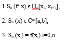
The Sn(f; x) function under consideration is called the local interpolation spline function when the following conditions are met:

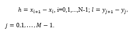
Based on the above conditions, we consider the construction of a local interpolation bicubic spline in the following D=[a,b]×[c,d] area. We can divide the area under consideration into N equal parts along the OX axis and M along the OY axis Δ=Δx×Δy. [1].

where steps h and l are selected as follows

Let we look at the grid below:

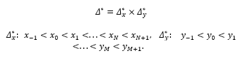
Δ_x^* for this case we make the field lookD^*=[a-h,b+h]×[c-l,d+l]. Δ^*- At the node points in the grid, the values of the function are known, i.e.:

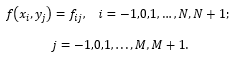
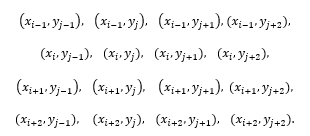
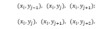
Based on the above values of the f(x,y)- function, we construct a local interpolation spline function for the field. To do this, we use the following 16 points.

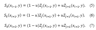
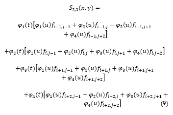
Our article in Comparative Analysis Spline Methods in Digital Processing of Signals in ASTESJ magazine describes the construction of a one-dimensional local cubic spline using 4 points [2]. Here, too, Zj(xi, j), Zj+1(xi, j) parabolas are constructed using the above points. Here x is fixed, i.e. at x=x_i the local interpolation bi cubic spline-function S_3 (x_i,y) has the following form:

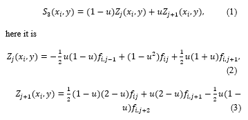Zj(xi, j), Zj+1(xi, j) parabolas are as follows

passes through node points. Substituting (2) and (3) into (1), we obtain the following after certain reductions:

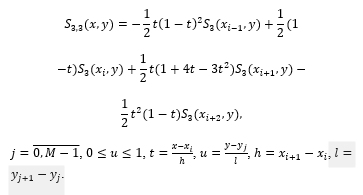
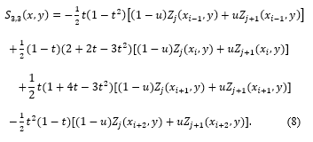
Based on the abovex=x_(i-1);”     ” x_(i+1);”      ” x_(i+2). In fixed cases, we create the following single-variable spline functions

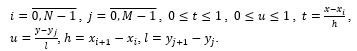
S3(xi-1, y), S3(xi, y), S3(xi+1, y) and S3(xi+2, y) Based on the one-variable cubic spline functions built above, after a certain compression, the following view of the following two-variable interpolation bicubic spline function is formed [3-7]:

S3(xi-1, y), S3(xi, y), S3(xi+1, y) and S3(xi+2, y) are generated by putting the values of the bicubic spline functions of a variable built above (8) [8-12].

Here it is

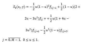
appears after a certain contraction (9).

here it is

(9) can be called a local interpolation bicubic spline function.
Digital processing of geophysical signals based on developed algorithms
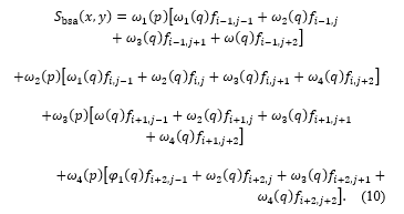
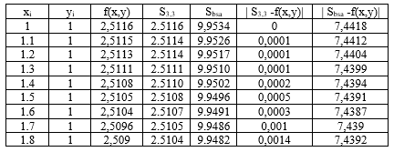
The proposed model considered the recovery of the signal obtained by aeromagnetic reconnaissance to determine the location of underground mineral resources, which is considered to be our current object (Table 1). Based on the above sequence, a local interpolation bicubic spline construction program was developed in the Matlab program environment and used in signal processing. The algorithm of this program is shown in Figure 3. We have shown the superiority of our model by comparing our developed model with the bicubic spline function S_bsa (10) model, which is based on the existing basic functions. Since it is not possible to cite all the known signals, we present the result in the following figures using the appearance of the signals in Table 1 (Figures 1-2). As can be seen from these pictures, it is clear from the S_3,3 and S_bsa spline functions that the degree of approximation of the S_3,3 we offer is high [13-16].

here it is

Figure 1: Graphical representation of the result obtained in the S_bsa function of the geophysical field
We used signals as real experimental data during our research. The obtained results are used to determine the location, size and amount of reserves of mineral resources by means of aerial magnetic intelligence. Of course, signal charts here use signals in the low frequency range from 10 to 50 kHz. Also, the distances between the nodes in the area under consideration must be equal [17-19].

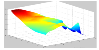Figure 2: Graphical representation of the result obtained in the S_3,3 function of the geophysical field

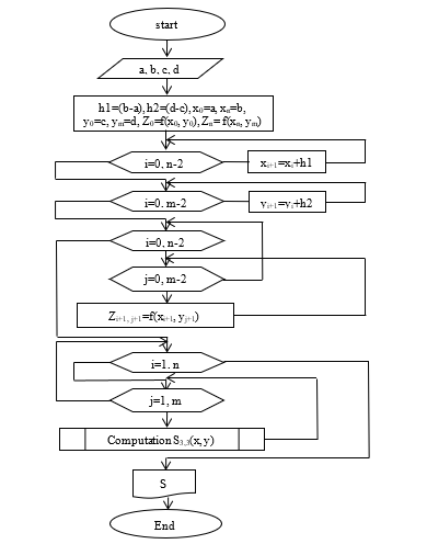Figure 3: Block diagram of a two-dimensional bicubic spline-function construction program.

Table 1: Initial values of the geophysical signal

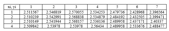
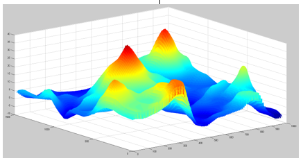Figure 4: Graphic representation of the result obtained by the S_bsa function with the geophysical field (0.1×0.1) step.

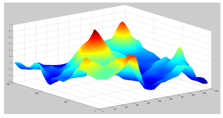Figure 5: Graphic representation of the result obtained by the S_3,3 function with the geophysical field (0.1×0.1) step.

Table 2: Results in error estimation in geophysical signal recovery.

Conclusion

The paper, a cubic spline built using a local base spline for digital signal processing and the local interpolation bicubic spline models we offer were selected. Construction details of the models are given. Two-dimensional local interpolation bicubic spline models provide high accuracy in digital processing of signals. As an example, the initial values of the geophysical signal given in Table 1 were numerically processed and the error results were obtained (Table 2). Based on the selected models, the results of geophysical signal recovery are presented graphically (Figures 1,2,3 and 4). Based on error results and graphs, it is effective to apply the two-dimensional local bicubic spline model in areas of geophysics and high accuracy.

1. Z. Xakimjon, K. Muslimjon, “Modeling of Geophysical Signals Based on the Secondorder Local Interpolication Splay-Function.,” in International Conference on Information Science and Communications Technologies: Applications, Trends and Opportunities, ICISCT 2019, 2019, doi:10.1109/ICISCT47635.2019.9011853.
2. Z. Xakimjon, A. Bunyod, “Biomedical signals interpolation spline models,” in International Conference on Information Science and Communications Technologies: Applications, Trends and Opportunities, ICISCT 2019, 2019, doi:10.1109/ICISCT47635.2019.9011926.
3. A.I. Grebennikov, “Isogeometric approximation of functions of one variable,” USSR Computational Mathematics and Mathematical Physics, 22(6), 1982, doi:10.1016/0041-5553(82)90095-7.
4. D. Singh, M. Singh, Z. Hakimjon, Geophysical application for splines, 2019, doi:10.1007/978-981-13-2239-6_7.
5. Selected Works of S.L. Sobolev, 2006, doi:10.1007/978-0-387-34149-1.
6. J.S. Lim, Two-dimensional signal and image processing, 1990.
7. Z. Zhengyu, “Digital processing of the polarization state of geophysical ULF signals,” Journal of Electronics (China), 11(3), 1994, doi:10.1007/BF02684833.
8. A. Kroizer, Y.C. Eldar, T. Routtenberg, “Modeling and recovery of graph signals and difference-based signals,” in GlobalSIP 2019 – 7th IEEE Global Conference on Signal and Information Processing, Proceedings, 2019, doi:10.1109/GlobalSIP45357.2019.8969536.
9. A.K. Takahata, E.Z. Nadalin, R. Ferrari, L.T. Duarte, R. Suyama, R.R. Lopes, J.M.T. Romano, M. Tygel, Unsupervised processing of geophysical signals: A review of some key aspects of blind deconvolution and blind source separation, IEEE Signal Processing Magazine, 29(4), 2012, doi:10.1109/MSP.2012.2189999.
10. X.H. Liu, Z.Y. Zhao, S.G. Xie, J.H. Liu, “Time-frequency analysis of geophysical signals based on Cohen distributions,” Dianbo Kexue Xuebao/Chinese Journal of Radio Science, 16(3), 2001.
11. B.H. Jansen, “ANALYSIS OF BIOMEDICAL SIGNALS BY MEANS OF LINEAR MODELING.,” Critical Reviews in Biomedical Engineering, 12(4), 1985.
12. D. Singh, M. Singh, Z. Hakimjon, Parabolic Splines based One-Dimensional Polynomial, 2019, doi:10.1007/978-981-13-2239-6_1.
13. R.O. Parker, “INTRODUCTION TO DIGITAL SIGNAL PROCESSING.,” J Eng Comput Appl, 2(3), 1988, doi:10.1201/9781439817391-5.
14. K. Daoudi, Iterated Function Systems and Some Generalizations: Local Regularity Analysis and Multifractal Modeling of Signals, 2010, doi:10.1002/9780470611562.ch9.
15. V. Graffigna, C. Brunini, M. Gende, M. Hernández-Pajares, R. Galván, F. Oreiro, “Retrieving geophysical signals from GPS in the La Plata River region,” GPS Solutions, 23(3), 2019, doi:10.1007/s10291-019-0875-6.
16. X. Wang, Z. Luo, B. Zhong, Y. Wu, Z. Huang, H. Zhou, Q. Li, “Separation and recovery of geophysical signals based on the Kalman Filter with GRACE gravity data,” Remote Sensing, 11(4), 2019, doi:10.3390/rs11040393.
17. P.S. Naidu, M.P. Mathew, Analysis of geophysical potential fields: a digital signal processing approach, 1998.
18. M.G. Molina, M.A. Cabrera, R.G. Ezquer, P.M. Fernandez, E. Zuccheretti, “Digital signal processing and numerical analysis for radar in geophysical applications,” Advances in Space Research, 51(10), 2013, doi:10.1016/j.asr.2012.07.032.
19. E.A. Robinson, T.S. Durrani, L.G. Peardon, “Geophysical signal processing.,” Geophysical Signal Processing., 1985, doi:10.1016/0264-8172(86)90037-1.

(Click Here)

(Click Here)