Face Recognition on Low Resolution Face Image With TBE-CNN Architecture
Face Recognition on Low Resolution Face Image With TBE-CNN Architecture
Volume 5, Issue 2, Page No 730-738, 2020
Author’s Name: Suharjitoa), Atria Dika Puspita
View Affiliations
Computer Science Department, Binus Graduate Program, Bina Nusantara University, 11480, Indonesia
a)Author to whom correspondence should be addressed. E-mail: suharjito@binus.edu
Adv. Sci. Technol. Eng. Syst. J. 5(2), 730-738 (2020); ![]() DOI: 10.25046/aj050291
DOI: 10.25046/aj050291
Keywords: Low Resolution, Face Recognition, Trunk-Branch Ensemble CNN

Export Citations
Face recognition in low resolution images has challenges in active research because face recognition is usually implemented in high resolution images (HR). In general, research leads to a combination of pre-processing and training models. Therefore, this study aims to classify low-resolution face images using a combination of pre-processing and deep learning. In addition, this study also aims to compare evaluation results based on differences in epoch values. In this research will use the Trunk Branch Ensemble – Convolutional Neural Network (TBE-CNN) as one of Convolutional Neural Network (CNN) architecture combined with the pre-processing method which is super resolution to get better accuracy compared to the state-of -art. Then the model is trained with different epoch values, that is 40 and 100, to compare the performance of the best classification. This study was evaluated by YTD Dataset. Based on the test results, this proposed method has achieved better results compared to the previous method, which gives an increase of 1%. After that, training results from different epoch values used also produce different accuracy at the training model but have no effect on validation and testing model. The training using epoch = 100 has an accuracy increase of 3% compared to training using epoch = 40 and the loss ratio obtained at the training is decreased by 20% compared to training at epoch = 40. Furthermore, optimization parameters are used and reducing computing time when training models and validation will be future research.
Received: 10 February 2020, Accepted: 04 March 2020, Published Online: 20 April 2020
1. Introduction
Face recognition is a biometric that is used to recognize human faces. According to [1], face recognition is known as an image system that is used to try to get the identity behind the video being played and protected faces that have been labeled. The face has several components, such as the eyes, nose and mouth. From face components, it can produce millions of face variations throughout the world. The one that make a differences of each person’s face are face shape, eyes, nose, mouth, and others. Based on the percentage of biometric usage described by [2], face recognition becomes the most usage on the system in Machine-Readable Travel Document MRTD with the graphic shown in Figure 1.
Face Recognition (FR) has become a very active research field due to the increasing demands of security, commercial applications and law enforcement applications [3]. For the examples of face recognition for security are finding someone’s identity based on a face photo, authenticating to login into a smartphone, and others. In addition, face recognition can also apply to surveillance cameras. Surveillance cameras are tools that help monitoring people in a room or area. Generally, face recognition is done on videos produced by surveillance cameras. But now, surveillance cameras have a low resolution, so the produced video also have low quality. This can be cause of face recognition accuracy tends to be low.
One of the face recognition methods that dealing with low-resolution problems and well-known today is deep learning. Deep learning is a new technology in machine learning that developed because along with the development of the GPU and the presence of big data has revives this technology. On the other hand, deep learning is a more accurate machine learning because they study the features of the data representation itself, so it minimize the require for programmer-based feature techniques [4].
One of the deep learning algorithms that can be used to face recognition is Convolutional Neural Network (CNN). CNN is a type of neural network that is used for image classification. The image here can be RGB or grayscale. CNN architecture is divided into 2, namely learning features and classification. There are 2 stages of learning on CNN, namely feed-forward and backpropagation.
 Figure 1: Comparison of the Most Widely Biometrics Used in MRTD Systems
In [5] the authors describe the four CNN architectures that are currently developi and be the subject of their research. The four architectures are Cross Correlation Mechanism CNN (CCM-CNN), TBE-CNN, HaarNet, and Canonical Face Representation CNN (CFR-CNN). From the accuracy obtained in the study proves that the TBE-CNN architecture and HaarNet have high accuracy for face recognition at low resolution. Previously, [6] conducted research using HaarNet on face recognition and compared it with Point-to-Set Correlation Learning (PSCL) architecture, Euclidean-to-Riemannian Metric (LERM) Learning, and TBE-CNN. And the results obtained for still-to-video prove that TBE-CNN is one of the best architectures for face recognition on low-resolution face images for still-to-video cases.
Trunk-Branch Architecture CNN (TBE- CNN) is one of the CNN architectures used to extract complementary features and patches around face landmarks through trunk and branches network. In the previous study, [7] has proposed two branch deep CNN method, which is a novel couple mapping using Deep Convolutional Neural Network (DCNN) and in this case using VGGFace pretrained model which is serves to mapping low and high-resolution face images into general space with non-linear transformations. And the proposed method has accuracy which is equal to 80.8% on the face size of 6 x 6 in the FERET dataset. After that, [3] proposed Deep Couple RestNet, which is a method whose architecture consists of 1 trunk using RestNet as the model and 2 branch networks (branch) using couple mapping to bring the distance between low and high resolution face images becoming certain resolutions and similar features will be placed in the new feature space. They also replaced the model in the trunk network with VGGFace and Light CNN for comparison and the results obtained were 93.6% for Coupled-ResNet, 83.7% for Coupled-VGGFace, and 80% for Coupled-Light CNN on the Labeled Face in The Wild (LFW) dataset for the size 8 x 8.
Adding pre-processing for face recognition at low resolutions is also widely used in research. According to [8] there are several pre-processing methods for solving low resolution face recognition problems such as Super Resolution (SR), feature-based representations likes local or global features, and structure-based representations likes coupled mappings, estimated resolution, and sparse representation. In the study, [3] used couple mapping on both branches to connect features on low and high-resolution face images into the same space. Likewise, [7] uses couple mapping on both branches and super resolution to construct low resolution face images to high resolution. This method will be better if combined with deep learning.
The results of this learning can be used by the police or other authorities to find the target person if there is a face matches from the supervisor’s surveillance camera. In this paper propose the development of the TBE-CNN architecture for face recognition at low resolution face images by combining methods in pre-processing and deep learning to perform face classifications on low-resolution face images. General research framework of this research defined as Figure 2.
![]() Figure 2: General Research Framework
Figure 2: General Research Framework
2. Related Work
On the pre-processing, [9] proposed a histogram alignment and image fusion approach. Generally, there’s two way for image fusion, one is fusion in spatial domain and other is fusion in frequency domain. This research using curvelet coefficient for representation face feature because it proven excellently performance in representing facial features.
Two years later, [10] proposed Resolution-Invariant Deep Network (RIDN) to study the resolution of invariant features. To make the comparison achievable, they raised the LR image resolution through interpolation methods such as Bicubic. They used cosine distance metric to get recognition results that can be an evaluation material of the proposed method. RIDN looks for uniform features that feasible to extract invariant feature resolutions then equations between samples computed using common distance metrics such as Euclidean and cosine through feature space. RIDN applies a deep convolutional network to study the resolution of invariant features. The size used is 60 x 55 for high resolution images and 30 x 24 for low resolution face images.
Then, [11] uses a Discriminant Correlation Analysis (DCA) that can resolve the mismatch length of vector features and the relationship between the corresponding features in an improved low and high-resolution face image. Before analyzing the features, researchers looked for 2 linear transformation matrices using Canonical Correlation Analysis (CCA). CCA is a method that processes valuable multi-data, which has been widely used to analyze the same relationship between two sets of variables. And the images used for observation are low resolution (32 x 32, 16 x 16, and 8 x 8) and high resolution (128 x 128) images.
Finally, [12] proposes Discriminative Multi-Dimensional Scaling (DMS) which is a functions to link high resolution face images and low resolution face images and Local-consistency-preserving DMS (LDMS) are functions to connect high resolution images with high resolution images too. The problem in this study is to find the appropriate distance for low resolution face images and high-resolution images. In this study they used couple mapping method to find 2 mappings or projecting of low-resolution face images and high-resolution face images into the same subspace. DMS is also used to find hidden subspaces that roughly their distance in spaces dist(h_i,h_j). h_i denoted as HR images that correspond to l_j. Gallery uses high-resolution images with test images that are larger than 32 x 32 and smaller than 16 x 16.
Table 1: Summary of State of Art
| Publication | Problem | Methods |
| [9] | Face recognition at low resolution for observation image sizes 32 x 32, 16 x 16, and 8 x 8. |
Face recognition at low resolution for observation image sizes 32 x 32, 16 x 16, and 8 x 8. |
| [10] |
Face recognition at low resolution to look for features in the same observation image with the gallery. |
Resolution-Invariant Deep Network (RIDN). |
| [11] |
Low-resolution face recognition taken from surveillance cameras for image size problems tested with those in the gallery is different from low resolution for observation images size 32 x 32, 16 x 16, 8 x 8 and high resolution with observation picture size 128 x 128. |
Use Canonical Correlation Analysis (CCA) and propose Discriminant Correlation Analysis (DCA). |
| [12] |
Low resolution face recognition to adjust the matrix in low and high-resolution face images with observational image sizes less than 32 x 32 and more than 16 x 16. |
Discriminative Multidimensional Scaling (DMS) and Local-consistency-preserved Discriminative Multidimensional Scaling (LDMS). |
| [3] | Face recognition at low resolutions with observational image sizes up to 8 x 8. | Deep Coupled ResNet, consist of one trunk network using ResNet and two branches using Coupled Mapping. |
| [7] | Face recognition at low resolutions with observational image sizes up to 6 x 6 sizes. | Two Branch with FECNN and SRFECNN (Combination of Super Resolution with FECNN). |
| [13] | Face recognition on video from surveillance cameras in the real world. The training dataset is taken from Face Detection on the surveillance camera. | CNN + Fine Tuning. |
| [14] | Face recognition in videos that have an unlimited variety of poses for still-to-video, video-to-still, and video-to-video cases. |
Trunk Branch Ensemble – Convolutional Neural Network (TBE-CNN). |
One of research that uses deep learning, [3] proposes Deep Couple RestNet. The architecture consists of 1 trunk and 2 branch networks. This network consists of convolutional layers, pooling, and 2 fully connected layers. The fully connected layer uses softmax and center-loss for interclass separation (classification). But to make a comparison, the authors replaced the model with VGGFace and LightCNN in the body tissue. The body network uses RestNet as its model while the branch network uses a couple mapping to close the distance between the low and high-resolution face images to a certain resolution and similar features will be placed in the new feature space.
Then [7] proposed the SRFECNN method which also offers high-resolution images because there is a super resolution CNN embedded in the architecture. The proposed method requires very little space, so it only requires a little memory. The proposed method is a novel couple mapping using a DCNN network (i.e. VGGNet) consisting of two DCNN branches for low and high-resolution face image maps into a common space with non-linear transformation.
The branch that handles high resolution images consists of 16 layers and the branch that handles low resolution face images consists of 5 super resolution layers connected to 14 layers (13 convolution layers and 1 fully-connected layer) and the third layer of fully connected layers will be used for so that the total classification for branches that deal with low-resolution face images is 19 layers. At the top branch which handles high resolution, 2 fully connected VGGnet layers removed so that the total layer at the top branch is 14 layers (13 convolution layers and 1 fully connected layer) of the total VGGnet layers.
This upper branch is called Feature Extraction Convolutional Neural Network (FECNN). Input image on the upper branch is 224 x 224 and other images than have other size will be done bicubic interpolation to an image size of 224 x 224. Bicubic interpolation used to resize the image as expected and softening the features of the image surface. The output are feature vectors with the number of elements is 4,096.
In lower branch that handles low resolution, the proposed method have 2 subnets. The first subnet called SRnet, using DCNN and the second subnet called FECNN, which is the same architecture as the upper branch. The output from SRnet will be the input for FECNN, which is an image with size 224 x 224. Input from the lower branch is a low-resolution face image that has been interpolated to size 224 x 224. The amount of weight used on SRFECNN is less than VGGnet, which is 141M.
The proposed method also uses Gradient Based Optimization to minimize the distance between low and high-resolution face images that are mapped into the same space by updating the DCNN weight via backpropagation on errors.
In addition, [13] used fine tuning in deep learning for face recognition. Fine tuning is a proposed method for constructing labelled datasets. Fine tuning is done on the face recognition model.
There are 3 stages in doing fine tuning. The first stage is to produce a rough dataset, such as collecting datasets obtained from surveillance cameras on lighting, poses, or expressions that vary by doing face detection and tracking. Then the second stage is refined dataset by labelling the dataset in each class using graph clustering from the VGG face model. Then the third stage, each class is purified by comparing its threshold values to eliminate duplication of datasets that are in each class. And the last step is to filter out classes, images that less than 100 classes will be eliminated.
Fine tuning is applied to VGG face models. The weight of VGG face model pre-training is done fine tuning by continuing back-propagation in the dataset. Only the fully connected layer that has been fine-tuned in the new dataset, so that makes the model fit the target.
At this time, [14] has proposed the architecture of the TBE-CNN. The architecture proposed also uses Mean Distance Regularization – Triplet Loss (MDR-TL) as a triplet loss function. This architecture consists of one body network and two branch networks. The body network used to study global features in face images while the branch network is used to study local features in face images. This architecture is evaluated by of still-to-video, video-to-still, and video-to-video case. All the previous work summarized on the Table 1.
3. Review Method
3.1. Low Resolution
According to [8], low resolution images is one of the issues on face recognition because ideally face recognition is trained and carried out with high-resolution images. The examples of low-resolution images are small image sizes, low image quality, lighting, unlimited poses (unconstrained), blurred images, or can be a combination of all of them. According to [15], they also said that low-resolution images taken from down-sampling did not present good low-resolution images and had a decreased performance in terms of face recognition. Low resolution face images occur due to several factors such as inaccuracies (miss-alignment), decreased resolution and various types of poses (noise affection), lacks in effective features, different resolutions when the learning process and image classification process (dimensional mismatch).
Generally, to solve low-resolution images is convert the low-resolution images to high-resolution images, then conduct training and classification of images with high-resolution images.
Low resolution images better used to classify images globally than using high-resolution images. There are 2 concepts to find out the best image resolution for face recognition, the one is determining the best image resolution and determining the minimum resolution (resolution threshold value) used. The low-resolution image has smaller size than 32 x 24 with an eye-to-eye distance of about 10 pixels taken from a surveillance camera that has 320 x 240 QVGA resolution without a cooperative subject and generally contains noise and blur.
3.2. Super Resolution
Super resolution or hallucination method is a technique to increase the resolution of low-sized images to high resolution. One method of super resolution is vision-oriented super resolution and recognition-oriented super resolution. Vision-oriented super resolution is a conventional super resolution technique that aims to obtain good visual reconstruction, but it’s not usually designed for the recognition purpose. Whereas recognition-oriented super resolution is a technique that aims to enhance visual images to suit the recognition purpose because along with reduced image resolution, general super resolution techniques (vision-oriented super resolution) become more vulnerable to unlimited pose variations.
3.3. Inception
Inception module is a module that acts as a multiple convolutional filter, where convolution is applied many times to the same input so it provide deeper convolution. Inception modules are generally illustrated by Figure 3. But the disadvantage of this inception is the large computational costs compared to simple convolution techniques.
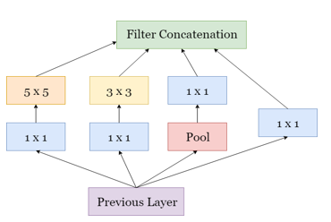 Figure 3: Common Inception Modules
3.4. Trunk-Branch Ensemble – Convolutional Neural Network Architecture (CNN)
CNN is a special type of neural network for data processing which has a topology known as a grid. The CNN name indicates a network that uses mathematical operations called convolution. According to experiments from [16] shows an increases in the number of parameters in the convolutional network layer without increasing the height of the convolution layer making the increase proven ineffective. After doing convolution, pooling is carried out to summarize the output of adjacent groups of neurons in the same kernel map. There is 2 type of pooling, one is max pooling and other is average pooling [17]. In this proposed model will using max pooling. Then fully connected will applied for classification. This layer has fixed dimensions and discards spatial coordinates. And this layer can be seen as a convolution with a kernel that covers the entire input region [18].
TBE-CNN is an one of CNN architecture for extracting complementary features and patches around facial landmarks through trunk and branch networks [5]. Trunk networks contain several layers to absorb global information and branch networks contain several layers to absorb local information thereby reducing computation and effective convergence. Trunk network are trained to study facial representations for holistic facial images, and each branch network is trained to study facial representations for patch images cutted from one facial component [13]. On [14], they combine GoogLeNet [19] architecture with TBE-CNN.
On TBE-CNN, [14] divides the layer to extract features into 3 parts, namely the low, middle, and high level layers. Low and middle level layers used to represent features that store local information, so that network entities and branch networks can exchange local information in the lower and middle layers. While the high-level layer serves features representation that store global information.
3.5. SGD Optimizer
Stochastic Gradient Descent (SGD) is an extension of gradient descent where it’s a modification of “batch” gradient descent and parameter updates are made after calculating a stochastic approximation of the gradient [20]. Gradient Descent calculate the gradient of cost function as much as number of training data. Many deep learning has powered by this algorithm. [21] explain that SGD have low memory usage, strong generalization ability, and incremental result. But SGD have sensitivity to learning rate hyperparameter. Based on research [22], they proven that SGD behaviour is also independent of the number of hidden units, as soon as this is large enough. Standard SGD notation are defined as follow:
![]() Where its optimized function from , η is a learning rate, and is a gradient at each step of . SGD reduce computational from Gradient Descent by multiply learning rate and cost gradient of 1 example at each training data without sum all gradient of cost function for each training data.
Where its optimized function from , η is a learning rate, and is a gradient at each step of . SGD reduce computational from Gradient Descent by multiply learning rate and cost gradient of 1 example at each training data without sum all gradient of cost function for each training data.
3.6. Softmax
The softmax loss function is a function used to represent the probability distribution of discrete variables with n possible values. The term “softmax” is a port-manteau of “soft” and “argmax” [23]. It is a typically good at optimizing the inter-class difference (i.e., separating different classes), but not good at reducing the intra-class variation (i.e., making features of the same class compact) [24]. The softmax function is most often used as the output of classifications. The softmax can be used within the model itself, if the model wants to choose one of different options for several internal variables. The softmax function is define by equations (6) [25].
![]() Where, is a vector input. Vector input might be negative value, or the sum is greater or less than one. So, after applying softmax function, the value will be range (0,1).
Where, is a vector input. Vector input might be negative value, or the sum is greater or less than one. So, after applying softmax function, the value will be range (0,1).
3.7. Ensemble Learning
Based on the understanding of [26], ensemble learning is a machine learning paradigm where several base learners or classifiers are trained to solve a problem, or one base leaner is trained several times to get the best accuracy or loss. Base learning is a model that will be combined in ensemble learning and the combination can be a neural network, deep learning, and others model, or it can be the same models. The concept of ensemble learning is generally illustrated in Figure 4.
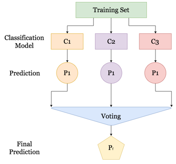 Figure 4: Common Ensemble Modules
The purpose of this combination is to produce better generalization performance compared to individual base learners. There are several methods in ensemble learning, the majority voting principle and the plurality voting principle [27]. Majority voting and plurality voting are ensemble learning methods where the way is to choose class labels or choose the highest accuracy (if the comparison uses accuracy) which is predicted from the whole base learner. The difference is the majority voting identically to binary classification while plurality voting is suitable for multiclass labels. Ensemble learning is denoted by equation (3) [27]:
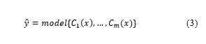
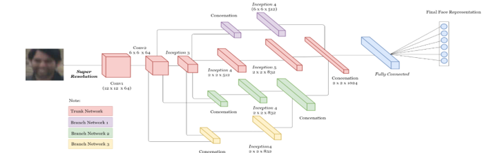 Figure 5: Common Ensemble Modules
Where the mode is the highest voting, C is the base learner or classifier and ŷ is the output that comes from the base learner or classifier that has the highest voting.
4. Result and Discussion
4.1. Dataset
In this study, the datasets used are YouTube Faces Database (YTD). The dataset used divided into training, validation, and testing with a portion of 70% for training, 20% for validation, and 10% for testing. Validation is done to avoid overfitting.
YouTube Faces Database (YTD) [28] is a dataset on face videos designed to study unlimited face recognition problems in video. This dataset contains 3,425 videos on 1,595 different subjects. All videos are downloaded from Youtube. The shortest clip duration is 48 frames, the longest clip is 6.070 frames, and the average length on the video clip is 181.3 frames. Total frame on this dataset is 621,126 image. In designing video datasets and benchmarks, [28] follow the example in the LFW image collection. YTD only contains video and provides still face image from a video that has been aligned on the same subject, whereas LFW only contains facial images that also on the same subject. The goal is to produce a collection of videos along with labels that indicate the identity of the people seen in each video. This dataset has enough blur, illumination, and lighting as the same as LFW dataset so YTD dataset able to verify algorithm performance for low resolution face recognition problem.
4.2. Pre-Processing
Pre-processing will be carried out on the TBE-CNN architecture development to be built. The pre-processing technique that will be used is super resolution. Super resolution is used to increase image resolution from low resolution face images to high resolution images so that the pixels in the image increase and the entire image used is clearly visible. The super resolution technique will be using bicubic interpolation function when resizing the image (face alignment). Bicubic interpolation is one of the super resolution techniques that can make the images surface smoother so that the face image can be used to make recognition.
4.3. Proposed Network Architecture
In the training phase, the face recognition model that will be used for TBE-CNN architecture development combined with pre-processing and model as shown in Figure 5. And this training will be using face training datasets and validation will be using face validation dataset. The dataset has been labeled before by their directories. The architecture consists of one trunk network and three branch networks. The trunk network will study global features. Whereas the branch networks will study the local features in image input. In the proposed architecture consist of a number of inceptions and use the Inception-v3 proposed by [29].
The branch two and three will be merging first before it will be merge to trunk and branch one. The parameter used described in Table 2 and the detail of model described in Table 3.
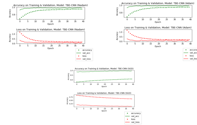 Figure 6: Training and Validation on TBE-CNN With Epoch 40
Table 2: Proposed Hyperparameter
| Dataset | Parameter | Value |
| YTD | Learning Rate | 1.0e-4 |
| Batch Size | 32 | |
| Optimizer | Adam, Nadam, and SGD | |
| Loss | categorical_crossentropy | |
|
Validation Step |
800 / batch size | |
| Activation | Softmax |
In the fully connected layer, it will use the softmax function as its activation function and the results of this fully connected layer will be evaluated by confusion matrix that has been applied by [30]. The training using the same epoch and combine with SGD as optimizer with momentum value is 0.9 (based on empirical study) and learning rate is 1.0e-4. For generate training, validation, and testing dataset, it using data augmented that rescaled to 1/255, zoom range is 0.2, shear range is 0.2, and horizontal flip is false.
The previous architecture consists of two branch and combine with couple mappings to project LR image from HR images. But for this architecture, it will add one branch network on the bottom and combine with Super Resolution as pre-processing method to increase images resolution.
In this study, there are 2 epoch values used in the model, i.e. 40 and 100. In training and validation at epoch = 40, it requires 3 times training with the same number of epochs to get optimal accuracy. And during the training process, the input trained using the GPU. For epoch = 100, the model is not trained in an ensemble and it run only once, so that this model training is called 3 Branch – Trunk Branch-CNN. For the model that was trained using epoch = 40, the model trained in an ensemble way, which is the model was trained 3 times with different optimizer, which is SGD, Adam, and Nadam. Both of these trainings using epoch = 100 and epoch = 40, started with random weight (initial weight).
4.4. Experiment Result and Discussion
By using the proposed model, the accuracy obtained is greater than that of state-of-art. However, based on the graph in Figure 5 shows that training and validation process with 3 different optimizers (ensemble learning).
Based on the training and validation using Adam optimizer shows that the accuracy at the last epoch in training was 98% while at the time of validation it was 99%. And for the loss in the last epoch in training by 20% while in validation by 18%. This is means that the difference in accuracy during training and validation is 1% and the difference in loss during training and validation is 2%.
Then in training and validation using Nadam optimizer shows that the accuracy in the last epoch in training was 97% while at the time of validation it was 99%. And for losses in the last epoch in training by 10% while in validation by 8%. This is means that the difference in accuracy during training and validation is 2% and the difference in loss during training and validation is 2%.
Table 3: Proposed Model Parameter
| Type (Name) |
Kernel Size / Stride |
Output Size | |
|
Low Level |
convolution (Conv1) |
7 x 7 / 2 | 12 x 12 x 64 |
| max pool | 2 x 2 / 2 | 6 x 6 x 64 | |
|
convolution (Conv2) |
3 x 3 / 1 | 3 x 3 x 192 | |
|
Middle Level |
inception (3a) | 3 x 3 x 256 | |
| inception (3b) | 3 x 3 x 480 | ||
| max pool | 2 x 2 / 2 | 3 x 3 x 480 | |
| High Level | inception (4a) | 3 x 3 x 512 | |
| inception (4b) | 3 x 3 x 512 | ||
| inception (4c) | 3 x 3 x 512 | ||
| inception (4d) | 3 x 3 x 528 | ||
| inception (4e) | 3 x 3 x 832 | ||
| max pool | 2 x 2 / 2 | 3 x 6 x 832 | |
| inception (5a) | 3 x 3 x 832 | ||
| inception (5b) | 3 x 3 x 1024 | ||
| concenation 1 | 3 x 3 x 1024 | ||
| concenation 2 | 3 x 3 x 1024 | ||
|
Fully Connected |
flatten | 1 x 36864 | |
| dense |
64 (dimension output) |
1 x 64 | |
| activation | 1 x 64 | ||
| dropout | 0.5 | 1 x 64 | |
| dense | 1591 (dimension output) | 1 x 1591 | |
| activation | 1 x 1591 |
Whereas in training and validation using SGD optimizer shows that the accuracy in the last epoch in training was 82% while at the time of validation it was 99%. And for losses in the last epoch in training by 60% while in validation by 5%. This is means that the difference in accuracy during training and validation is 17% and the difference in loss during training and validation is 55%.
From the results of these experiments, it can be concluded that training using Adam’s optimizer provides the best results compared to the other 2 optimizers, both in terms of accuracy and loss that can be obtained. And SGD optimizer gives the lowest results compared to 2 other optimizers.
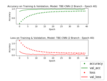 Figure 7: Training and Validation on TBE-CNN with 2 Branch
From the highest accuracy based on training using the ensemble approach, the accuracy will be compared with the model using 2 branches. In Figure 7 shows that the accuracy at the last epoch in training was 95% while at the time of validation it was 99%. And for the loss in the last epoch in training by 25% while in validation by 3%. This is means that the difference in accuracy during training and validation is 4% and the difference in loss during training and validation is 22%.
Table 4: Comparison Accuracy
| Method | Accuracy (%) |
| TBE-CNN (2 Branch) | 99% |
|
3 Branch-Trunk Branch Ensemble-CNN (Epoch 40 – Optimizer Adam) |
100% |
|
3 Branch-Trunk Branch Ensemble-CNN (Epoch 40 – Optimizer Nadam) |
100% |
|
3 Branch-Trunk Branch Ensemble-CNN (Epoch 40 – Optimizer SGD) |
99% |
|
3 Branch-Trunk Branch-CNN (Epoch 100) |
99% |
Because SGD provides the lowest accuracy, the next research is continued by changing the epoch value to 100 and using SGD as an optimizer model, the rest use the same parameters as the parameters used at epoch = 40. The change in epoch value is intended to compare training results, validation, and testing obtained when using different epochs. At epoch = 100, the weight used originates from initialization or does not use the weight of the training results and validation at epoch = 40. Based on the graph in Figure 7 shows that the accuracy at the last epoch in training using epoch = 100 was 85% while at the time of validation it was 99%. And for the loss in the last epoch in training by 40% while in validation by 5%. This is means that the difference in accuracy during training and validation is 14% and the difference in loss during training and validation is 35%.
When compared with the results of accuracy in training and validation using epoch = 40, the comparison of accuracy in training can be increased by 3%, while the accuracy ratio for validation is 0% (none). Then, for the comparison of accuracy obtained during training that is decreased by 20% and the loss ratio at the time of validation is 0% (none). On the testing phase, the model is tested using a confusion matrix. From the ensemble learning test results on Table 4 proved that the optimizer Adam and Nadam provide the best accuracy compared to other optimizers. In addition, epoch comparisons show on Table 5 do not provide significant accuracy differences during validation and testing, but on the Figure 6 and Figure 8 shows that epoch comparison provides increased accuracy and loss in training.
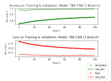 Figure 8: Training and Validation on TBE-CNN with 2 Branch
On the comparison to state-of-art, the accuracy obtained from the experimental results will be compared with [14]. The architecture also used a YTD dataset with an input size of 24 x 24. From the accuracy comparison in Table 4 it can be concluded that the 3 Branch – Trunk Branch Ensemble-CNN model is able to improve the accuracy of the previous method and the improvement is 1%.
5. Conclusion
In this paper proposed a method Trunk branch Ensemble-CNN and Trunk Branch-CNN with super resolution as pre-processing. The architecture consists of inception-v3 by GoogLeNet. The proposed architecture compared to previous architecture and evaluated by YTD dataset. And the results show that Adam and Nadam optimizer give the best accuracy on testing in ensemble learning and the proposed method provides better accuracy compared to state-of-art. Then, different epoch can affect the training performance results but not give significant improvement for validation and testing result. Furthermore, the optimization of parameter used and reduce computational time when model training and validation will be future work.
Conflict of Interest
We declare that we have no affiliations with or involvement in any organization or entity with any financial interest (such as honoraria; educational grants; participation in speakers’ bureaus; membership, employment, consultancies, stock ownership, or other equity interest, and expert testimony or patent-licensing arrangements), or non-financial interest (such as personal or professional relationships, affiliations, knowledge or beliefs) in the subject matter or materials discussed in this manuscript.
- K. Bhavani et al., Real time Face Detection and Recogni tion in Video Surveillance, Int. Res. J. Eng. Technol., vol. 4, pp. 1562–1565 (2017)
- T. Huang, Z. Xiong, and Z. Zhang, Face recognition applications. Springer, London (2011)
- Z. Lu, X. Jiang, and A. Kot, Deep Coupled ResNet for Low-Resolution Face Recognition, IEEE Signal Process. Lett., vol. 25, pp. 526–530 (2018)
- J. S. Patil, Deep Learning in Low Resolution Image Recog nition, Vishwakarma J. Eng. Res., vol. 1, pp. 101–107 (2017)
- S. Bashbaghi, E. Granger, R. Sabourin, and M. Parchami, Deep Learning Architectures for Face Recognition in Video Surveillance, arXiv Prepr. arXiv1802.09990, pp. 1–21 (2018)
- M. Parchami, S. Bashbaghi, and E. Granger, Video-based face recognition using ensemble of haar-like deep convolutional neural networks, 2017 Int. Jt. Conf. Neural Networks, pp. 4625–4632 (2017)
- E. Zangeneh, M. Rahmati, and Y. Mohsenzadeh, Low Resolution Face Recognition Using a Two-Branch Deep Convolutional Neural Network Architecture, Comput. Vis. Pattern Recognit., vol. 4, pp. 1562–1565 (2017)
- Z. Wang, Z. Miao, Q. M. Jonathan Wu, Y. Wan, and Z. Tang, Low-resolution face recognition: A review, Vis. Comput., vol. 30, pp. 359–386 (2014)
- X. Xu, W. Liu, and L. Li, Low Resolution Face Recognition in Surveillance Systems, J. Comput. Commun.. Technol., vol. 2, pp. 70–77 (2014)
- D. Zeng, H. Chen, and Q. Zhao, Towards resolution invariant face recognition in uncontrolled scenarios, 2016 International Conference on Biometrics (2016)
- M. Haghighat and M. Abdel-Mottaleb, Lower Resolution Face Recognition in Surveillance Systems Using Discriminant Correlation Analysis, 2017 12th IEEE Int. Conf. Autom. Face Gesture Recognit., pp. 912–917 (2017)
- F. Yang, W. Yang, R. Gao, and Q. Liao, Discriminative Multidimensional Scaling for Low-Resolution Face Recognition, IEEE Signal Process. Lett., vol. 25, pp. 388–392 (2018)
- Y. Wang, T. Bao, C. Ding, and M. Zhu, Face Recognion in Real-world Surveillance Videos with Deep Learning Method, 2017 2nd Int. Conf. Image, Vis. Comput., pp. 239–243 (2017)
- C. Ding and D. Tao, Trunk-Branch Ensemble Convolutional Neural Networks for Video-Based Face Recognition, IEEE Trans. Pattern Anal. Mach. Intell., vol. 40, pp. 1002–1014 (2018)
- P. Li, L. Prieto, D. Mery, and P. Flynn, Face Recognition in Low Quality Images: A Survey, Comput. Vis. Pattern Recognit., pp. 1–15 (2018)
- I. J. Goodfellow, Y. Bulatov, J. Ibarz, S. Arnoud, and V. Shet, Multi-digit Number Recognition from Street View Imagery using Deep Convolutional Neural Networks, Comput. Vis. Pattern Recognit., pp. 1–13 (2013)
- K. He, X. Zhang, S. Ren, and J. Sun, Deep Residual Learning for Image Recognition, 2016 IEEE Conf. Comput. Vis. Pattern Recognit., pp. 770–778 (2016)
- J. Long, E. Shelhamer, and T. Darrell, Fully convolutional networks for semantic segmentation, Proc. IEEE Comput. Soc. Conf. Comput. Vis. Pattern Recognit., vol. 07, pp. 3431–3440 (2015)
- C. Szegedy et al., Going deeper with convolutions, Proc. IEEE Comput. Soc. Conf. Comput. Vis. Pattern Recognit., vol. 07, pp. 1–9 (2015)
- S. Balaban, Deep learning and face recognition: the state of the art, Biometric Surveill. Technol. Hum. Act. Identif. XII, vol. 9457, pp. 94570B (2015)
- J. Perla, Notes on AdaGrad Regret of AdaGrad, arXiv, pp. 1–5 (2014)
- S. Mei, A. Montanari, and P.-M. Nguyen, A mean field view of the landscape of two-layer neural networks, Proc. Natl. Acad. Sci., vol. 115, pp. E7665–E7671 (2018)
- B. Gao and L. Pavel, On the Properties of the Softmax Function with Application in Game Theory and Reinforcement Learning, pp. 1–10 (2017)
- F. Wang, J. Cheng, W. Liu, and H. Liu, Additive Margin Softmax for Face Verification, IEEE Signal Process. Lett., vol. 25, pp. 926–930 (2018)
- I. Goodfellow, Y. Bengio, and A. Courville, Deep learning (Vol. 1). MIT press, Cambridge (2016)
- Z. Zhou, Ensemble Learning, pp. 1–5
- S. Raschka, Python Machine Learning. PACKT, Birmingham (2015)
- L. Wolf, T. Hassner, and I. Maoz, Face recognition in unconstrained videos with matched background similarity, Proc. IEEE Comput. Soc. Conf. Comput. Vis. Pattern Recognit., pp. 529–534 (2011)
- C. Szegedy, V. Vanhoucke, S. Ioffe, J. Shlens, and Z. Wojna, Rethinking the Inception Architecture for Computer Vision, Comput. Vis. Pattern Recognit. (2015)
- S. Turgut, M. Dagtekin, and T. Ensari, Microarray breast cancer data classification using machine learning methods, 2018 Electr. Electron (2018)