Plane wave propagation in a 3D anisotropic half-space under Green-Naghdi theory II

Chakraborty, S.; Mandal, S. C.; Das, A. K.; Sarkar, N.; Lahiri, A.

doi:10.21595/mme.2016.17621

Mathematical Models in Engineering

Browse Journal

Submit article

Published: 31 December 2016

Check for updates

Plane wave propagation in a 3D anisotropic half-space under Green-Naghdi theory II

S. Chakraborty¹

S. C. Mandal²

A. K. Das³

N. Sarkar⁴

A. Lahiri⁵

^{1, 2, 5}Department of Mathematics, Jadavpur University, Kolkata, 700032, India

³Department of Geology, Asutosh College, 92, S. P. Mukherjee Road, Kolkata, 700026, India

⁴Department of Applied Mathematics, University of Calcutta, Kolkata, 700009, India

Corresponding Author:

N. Sarkar

Cite the article Download PDF

Downloads 1657

CrossRef Citations 2

Abstract

In this paper, the theory of coupled thermoelasticity in three dimension is employed for triclinic half-space, subjected to time dependent heat source on the boundary of the space which is traction free and is considered in the context of Green-Naghdi model of type II (thermoelasticity without energy dissipation) of generalized thermoelasticity. Normal mode analysis is used to the non-dimensional coupled equations. Finally, the resulting equations are written in the form of a vector-matrix differential equation which is then solved by eigenvalue approach. Numerical results for the temperature, thermal stresses, and displacements are presented graphically and analyzed. Mathematical results shown in thermoelastic curves were supplemented by tectonic movements of elastic lithospheric plates.

1. Introduction

The classical uncoupled theory of thermoelasticity, predicts two phenomena not consistent with experimental results. The heat conduction equation of this theory i) does not contain any elastic terms, but the fact is that the elastic changes produces heat effects and ii) the heat conduction equation is of parabolic type predicting infinite speeds of propagation for heat waves, which means that the theory classical of thermoelasticity (CT) predicts finite for predominantly elastic disturbances but an infinite speed for predominantly thermal disturbances, which are coupled together. This means that a part of every solution of the equations extends to infinity. To overcome this paradox inherent in the theory of classical uncoupled theory of thermoelasticity, Biot [1] introduced the theory of coupled thermoelasticity.

To eliminate the second shortcoming Lord and Shulman [2] (L-S model) introduce a theory of generalized thermoelasticity with one relaxation time parameter, by modification of Fourier’s law, replaced heat flux and its time derivatives. In L-S model the heat conduction equation is hyperbolic type and is closely connected with the theories of “second sound”. This theory was extended for anisotropic body by Dhaliwal and Sherief [3]. The uniqueness of the solutions for this theory was proved under different conditions by Ignaczak [4, 5]. Green and Lindsay [6] (G-L model) modified not only heat conduction equation but also equation of motion in the coupled theory without violating Fourier’s law by introducing two relaxation time parameters. Along with the theories, Green and Naghdi [7-9] (G-N model) also proposed another three generalized theories of thermoelasticity by introducing “thermal displacement gradient” among the independent constitutive variables and named as Type I, II and III. Among these models, type I [7] is same as classical heat equation which is based on Fourier’s law where the theories are linearized. The type II [9] and type III [8] model permit finite speed of wave propagation. The basic difference of type II from type I and type III is that it does not contain dissipation of thermal energy whereas type III contains dissipation of energy. The type II and Type III are also known as thermoelasticity without energy dissipation (TEWOED) and thermoelasticity with energy dissipation (TEWED). Several investigations relating to TEWOED theory have been studied by Roy Choudhury and Bandyopadhyay [10], Roy Choudhury and Dutta [11], Sharma and Chouhan [12], Chandrasekharaiah and Srinath [13], Sarkar and Lahiri [14] and Bachher et al. [MME15]. The effect of magnetic field in generalized thermoelasticity with internal heat source in half space was investigated by Othman et al. [16]. Pal and Acharya [17] studied the effects of inhomogeneity on the surface waves in anisotropic media. Recently, Pal et al. [18] investigated the wave propagation in an inhomogeneous anisotropic generalized thermoelastic solid. They have also shown by graphically that quasi-P wave, quasi-S wave and thermal wave are discontinuous at certain angle and with a jump as well.

We know that materials in the earth are not homogeneous although their elastic properties vary with depth from one region to another. The variation may be gradual; there are also discontinuities that separate media with different densities and elastic properties. Anisotropy causes the largest variation of seismic velocities and changes in the direction of seismic waves. Achenbach [19] studied reflection and transmission of wave in infinite elastic plate. Several investigations relating to reflection and transmission of elastic waves in anisotropic media have been studied by Nayfeh [20], Pal and Chattopadhyay [21], Chattopadhyay and Rogerson [22], Sharma [23] and Chattopadhyay et al. [24]. Mensch and Rasolofosaon [25] studied the elastic wave velocities in anisotropic media, generalizing Thomson’s parameters, $δ$ and $γ$ . Abbas and Othman [26] investigated the propagation of plane waves in fiber-reinforced, anisotropic half-space under effect of hydrostatic initial in L-S model. The analysis of Lame waves in anisotropic thin plates in generalized thermoelasticity was discussed by Verma [27]. Zhou and Greenhalgh [28], Grechka [29] studied elastic wave group velocities for (generalized) anisotropic medium. The petrophysical study of velocity of waves in anisotropic shale was analyzed by Vernik and Liu [30], Kumar and Gupta [31] investigated the plane wave propagation in anisotropic thermoelastic medium having fractional order derivative and void in the context of three- phase lag model and two phase lag model. Recently Othman et.al. [32] studied the effect of rotation on three dimensional generalized thermoelasticity in the context of Green-Nagdhi type II for homogeneous isotropic elastic half space.

The thermo-elastic stress behavior and strain calculations due to time-dependent thermal perturbation in homogeneous plates have significant applications in tectonic movements of more homogeneous rigid plates e.g., basaltic oceanic plates subjected to heat sources of hot magmatic plumes of deeper mantle origin. Thus the deduction and modifications of thermo-elastic stresses in proportion to the degree of reheating of the elastic lithosphere are explained in various hotspot thermal models (Zhu and Wiens [33]). The aim of the present research article to study the distribution of stresses, strains and temperature for an anisotropic half space subjected to a time dependent heat source on the boundary of the space which is traction free in the context of Green-Naghdi model – II. Normal mode analysis technique and eigenvalue approach have been used to solve the problem. Finally, numerical results are presented graphically and analyzed. Some applications have been also given.

2. Basic equations

In the absence of body forces and inner heat sources, the field equations for linear thermoelastic homogeneous anisotropic body in the context of Green-Nagdhi model II [9], Othman et al. [32] are as follows:

The equations of motion:

1

τ_{i j, j} = ρ {\ddot{u}}_{i} .

Heat- conduction equation of Green- Nagdhi theory of type II:

2

k_{i j}^{*} θ,_{i j} = ρ c_{E} \ddot{θ} + θ_{0} b_{i j} {\ddot{u}}_{i, j} .

The Duhamel-Neumann constitutive equations are:

3

τ_{i j} = c_{i j k l} e_{k l} - β_{i j} θ δ_{i j} .

Strain – displacement relation:

4

e_{i j} = \frac{1}{2} (u_{i, j} + u_{j, i}), u_{i, j} = \frac{\partial u_{i}}{\partial x_{j}} .

The comma notation is used for derivatives with respect to space variables $x_{i}$ and superimposed dot represents time differentiation.

3. Formulation of the problem

We shall consider a triclinic linear thermoelastic anisotropic half-space solid which fills the region $Ω = \{(x_{1}, x_{2}, x_{3}) : 0 \leq x_{1} < \infty, - \infty < x_{2} < \infty, - \infty < x_{3} < \infty\}$ and subjected to time dependent heat sources on the boundary plane to the surface $x_{1} = 0$ . The body is initially at rest and the surface $x_{1} = 0$ is assumed to be traction free.

For three dimensional plane waves in a homogeneous anisotropic elastic medium, the components of displacement vector have the form:

5

u_{i} = u_{i} (x_{1}, x_{2}, x_{3}, t), i = 1,2, 3,

where $t$ is the time variable and $x_{i}$ ( $i =$ 1, 2, 3) denotes the respective orthogonal Cartesian co-ordinate axes. Using Hooke’s law, the stress-strain-temperature relations in a triclinic medium can be written as follows:

6

τ_{11} = c_{11} e_{11} + c_{12} e_{22} + c_{13} e_{33} + 2 (c_{14} e_{23} + c_{15} e_{13} + c_{16} e_{12}) - β_{11} θ,

τ_{22} = c_{21} e_{11} + c_{22} e_{22} + c_{23} e_{33} + 2 (c_{24} e_{23} + c_{25} e_{13} + c_{26} e_{12}) - β_{22} θ,

τ_{33} = c_{31} e_{11} + c_{32} e_{22} + c_{33} e_{33} + 2 (c_{34} e_{23} + c_{35} e_{13} + c_{36} e_{12}) - β_{33} θ,

τ_{23} = c_{41} e_{11} + c_{42} e_{22} + c_{43} e_{33} + 2 (c_{44} e_{23} + c_{45} e_{13} + c_{46} e_{12}),

τ_{13} = c_{51} e_{11} + c_{52} e_{22} + c_{53} e_{33} + 2 (c_{54} e_{23} + c_{55} e_{13} + c_{56} e_{12}),

τ_{12} = c_{61} e_{11} + c_{62} e_{22} + c_{63} e_{33} + 2 (c_{64} e_{23} + c_{65} e_{13} + c_{66} e_{12}) .

The equations of motion in absence of body forces and heat sources are as follows:

7

τ_{11,1} + τ_{12,2} + τ_{13,3} = ρ {\ddot{u}}_{1},

τ_{21,1} + τ_{22,2} + τ_{23,3} = ρ {\ddot{u}}_{2},

τ_{31,1} + τ_{32,2} + τ_{33,3} = ρ {\ddot{u}}_{3} .

With the help of Eq. (5) and (6), equations of motion (7) become:

8

ρ {\ddot{u}}_{1} = (c_{11} u_{1,11} + c_{66} u_{1,22} + c_{55} u_{1,33}) + 2 (c_{16} u_{1,12} + c_{15} u_{1,13} + c_{56} u_{1,23})

+ (c_{16} u_{2,11} + c_{26} u_{2,22} + c_{45} u_{2,33} + (c_{12} + c_{66}) u_{2,12} + (c_{14} + c_{56}) u_{2,13}

+ (c_{46} + c_{25}) u_{2,23}) + (c_{15} u_{3,11} + c_{46} u_{3,22} + c_{35} u_{3,33} + (c_{14} + c_{56}) u_{3,12})

+ (c_{13} + c_{55}) u_{3,13} + (c_{36} + c_{45}) u_{3,23}) - β_{11} θ_{, 1},

ρ {\ddot{u}}_{2} = (c_{16} u_{1,11} + c_{26} u_{1,22} + c_{45} u_{1,33} + (c_{12} + c_{66}) u_{1,12}

+ (c_{14} + c_{56}) u_{1,13} (c_{46} + c_{25}) u_{1,23}) + (c_{66} u_{2,11} + c_{22} u_{2,22} + c_{44} u_{2,33})

+ 2 (c_{26} u_{2,12} + c_{46} u_{2,13} + c_{24} u_{2,23}) + (c_{56} u_{3,11} + c_{24} u_{3,22} + c_{34} u_{3,33}

+ (c_{46} + c_{25}) u_{3,12} + (c_{36} + c_{45}) u_{3,13} + (c_{23} + c_{44}) u_{3,23}) - β_{22} θ_{, 2},

ρ {\ddot{u}}_{3} = (c_{15} u_{1,11} + c_{46} u_{1,22} + c_{35} u_{1,33} + (c_{56} + c_{14}) u_{1,12}

+ (c_{55} + c_{13}) u_{1,13} + (c_{45} + c_{36}) u_{1,23}) + (c_{56} u_{2,11} + c_{24} u_{2,22} + c_{34} u_{2,33}

+ (c_{25} + c_{46}) u_{2,12} + (c_{45} + c_{36}) u_{2,13} + (c_{44} + c_{23}) u_{2,23})

+ (c_{55} u_{3,11} + c_{44} u_{3,22} + c_{33} u_{3,33}) + 2 (c_{45} u_{3,12} + c_{35} u_{3,13} + c_{34} u_{3,23}) - β_{33} θ_{, 3} .

The generalized heat conduction Eq. (2) is written as:

9

k_{11}^{*} θ_{, 11} + k_{22}^{*} θ_{, 22} + k_{33}^{*} θ_{, 33} = ρ c_{E} \ddot{θ} + θ_{0} (b_{11} {\ddot{u}}_{1,1} + b_{22} {\ddot{u}}_{2,2} + b_{33} {\ddot{u}}_{3,3}) .

To transform the above equations in non-dimensional forms, we introduce the following non-dimensional variables:

10

{x'}_{i} = \frac{1}{l} x_{i}, {u'}_{i} = \frac{ρ {c_{1}}^{2}}{l b_{11} θ_{0}} u_{i}, t^{'} = \frac{c_{1}}{l} t, θ^{'} = \frac{1}{θ_{0}} θ, {τ'}_{i j} = \frac{1}{b_{11} θ_{0}} τ_{i j}, c_{1}^{2} = \frac{c_{11}}{ρ},

where $l$ is some standard length.

Using the parameters defined in Eq. (10), the non-dimensional forms of the equations of motion, heat conduction equation and stress components can be obtained as (omitting primes for convenience):

11

{\ddot{u}}_{1} = (u_{1,11} + \frac{c_{66}}{c_{11}} u_{1,22} + \frac{c_{55}}{c_{11}} u_{1,33}) + 2 (\frac{c_{16}}{c_{11}} u_{1,12} + \frac{c_{15}}{c_{11}} u_{1,13} + \frac{c_{56}}{c_{11}} u_{1,23})

+ (\frac{c_{16}}{c_{11}} u_{2,11} + \frac{c_{26}}{c_{11}} u_{2,22} + \frac{c_{45}}{c_{11}} u_{2,33}) + (\frac{(c_{12} + c_{66})}{c_{11}} u_{2,12} + \frac{(c_{14} + c_{56})}{c_{11}} u_{2,13}

+ \frac{(c_{46} + c_{25})}{c_{11}} u_{2,23}) + (\frac{c_{15}}{c_{11}} u_{3,11} + \frac{c_{46}}{c_{11}} u_{3,22} + \frac{c_{35}}{c_{11}} u_{3,33} + \frac{(c_{14} + c_{56})}{c_{11}} u_{3,12}

+ \frac{(c_{13} + c_{55})}{c_{11}} u_{3,13} + \frac{(c_{36} + c_{45})}{c_{11}} u_{3,23}) - θ_{, 1},

{\ddot{u}}_{2} = (\frac{c_{16}}{c_{11}} u_{1,11} + \frac{c_{26}}{c_{11}} u_{1,22} + \frac{c_{45}}{c_{11}} u_{1,33} + \frac{(c_{12} + c_{66})}{c_{11}} u_{1,12} + \frac{(c_{14} + c_{56})}{c_{11}} u_{1,13}

+ \frac{(c_{46} + c_{25})}{c_{11}} u_{1,23}) + (\frac{c_{66}}{c_{11}} u_{2,11} + \frac{c_{22}}{c_{11}} u_{2,22} + \frac{c_{44}}{c_{11}} u_{2,33})

+ 2 (\frac{c_{26}}{c_{11}} u_{2,12} + \frac{c_{46}}{c_{11}} u_{2,13} + \frac{c_{24}}{c_{11}} u_{2,23}) + (\frac{c_{56}}{c_{11}} u_{3,11} + \frac{c_{24}}{c_{11}} u_{3,22} + \frac{c_{34}}{c_{11}} u_{3,33}

+ \frac{(c_{46} + c_{25})}{c_{11}} u_{3,12} + \frac{(c_{36} + c_{45})}{c_{11}} u_{3,13} + \frac{(c_{23} + c_{44})}{c_{11}} u_{3,23}) - b_{2} θ_{, 2},

{\ddot{u}}_{3} = (\frac{c_{15}}{c_{11}} u_{1,11} + \frac{c_{46}}{c_{11}} u_{1,22} + \frac{c_{35}}{c_{11}} u_{1,33} + \frac{(c_{56} + c_{14})}{c_{11}} u_{1,12} + \frac{(c_{55} + c_{13})}{c_{11}} u_{1,13}

+ \frac{(c_{45} + c_{36})}{c_{11}} u_{1,23}) + (\frac{c_{56}}{c_{11}} u_{2,11} + \frac{c_{24}}{c_{11}} u_{2,22} + \frac{c_{34}}{c_{11}} u_{2,33} + \frac{(c_{25} + c_{46})}{c_{11}} u_{2,12}

+ \frac{(c_{45} + c_{36})}{c_{11}} u_{2,13} + \frac{(c_{44} + c_{23})}{c_{11}} u_{2,23}) + (\frac{c_{55}}{c_{11}} u_{3,11} + \frac{c_{44}}{c_{11}} u_{3,22} + \frac{c_{33}}{c_{11}} u_{3,33})

+ 2 (\frac{c_{45}}{c_{11}} u_{3,12} + \frac{c_{35}}{c_{11}} u_{3,13} + \frac{c_{34}}{c_{11}} u_{3,23}) - β_{3} θ_{, 3},

12

c_{T}^{2} (θ_{, 11} + k_{2} θ_{, 22} + k_{3} θ_{, 33}) = \ddot{θ} + ε_{1} ({\ddot{u}}_{1,1} + β_{2} {\ddot{u}}_{2,2} + β_{3} {\ddot{u}}_{3,3}),

13

τ_{11} = \frac{1}{c_{11}} [c_{11} e_{11} + c_{12} e_{22} + c_{13} e_{33} + 2 (c_{14} e_{23} + c_{15} e_{13} + c_{16} e_{12})] - θ,

τ_{22} = \frac{1}{c_{11}} [c_{21} e_{11} + c_{22} e_{22} + c_{23} e_{33} + 2 (c_{24} e_{23} + c_{25} e_{13} + c_{26} e_{12})] - β_{2} θ,

τ_{33} = \frac{1}{c_{11}} [c_{31} e_{11} + c_{32} e_{22} + c_{33} e_{33} + 2 (c_{34} e_{23} + c_{35} e_{13} + c_{36} e_{12})] - β_{3} θ,

τ_{23} = \frac{1}{c_{11}} [c_{41} e_{11} + c_{42} e_{22} + c_{43} e_{33} + 2 (c_{44} e_{23} + c_{45} e_{13} + c_{46} e_{12})],

τ_{13} = \frac{1}{c_{11}} [c_{51} e_{11} + c_{52} e_{22} + c_{53} e_{33} + 2 (c_{54} e_{23} + c_{55} e_{13} + c_{56} e_{12})],

τ_{12} = \frac{1}{c_{11}} [c_{61} e_{11} + c_{62} e_{22} + c_{63} e_{33} + 2 (c_{64} e_{23} + c_{65} e_{13} + c_{66} e_{12})],

where:

{c_{T}}^{2} = \frac{k_{11}^{*}}{ρ c_{E} {c_{1}}^{2}}, ε_{1} = \frac{b_{11}^{2} q_{0}}{r C_{11} C_{E}}, ε_{r} = ε_{1} β_{r r}, k_{r} = \frac{k_{r r}^{*}}{k_{11}^{*}}, β_{r} = \frac{β_{r r}}{β_{11}}, r = 2,3 .

4. Normal mode analysis: Formulation of vector–matrix differential equation

For the solution of the Eqs. (11) and (12), the physical variables can be decomposed in terms of normal modes [14] in the following form:

14

[u_{1}, u_{2}, u_{3}, e_{i j}, θ, τ_{i j}] (x_{1}, x_{2}, x_{3}, t) = [u_{_{1}}^{*}, u_{_{2}}^{*}, u_{_{3}}^{*}, e_{i j}^{*}, θ^{*}, τ_{i j}^{*}] (x_{1}) e^{ω t + i (a x_{2} + b x_{3})},

where $i = \sqrt{- 1}$ , $ω$ is the angular frequency and $a$ , $b$ are the wave numbers along $x_{2}$ and $x_{3}$ directions respectively.

Substituting from Eq. (14) in Eqs. (11)-(13), we obtain (omitting ‘*’ for convenience):

15

u_{1,11} + a_{11} u_{1,1} + a_{12} u_{1} + a_{21} u_{2,11} + a_{22} u_{2,1} + a_{23} u_{2} + a_{31} u_{3,11}

+ a_{32} u_{3,1} + a_{33} u_{3} - θ_{, 1} = 0,

16

b_{11} u_{1,11} + b_{12} u_{1,1} + b_{13} u_{1} + u_{2,11} + b_{21} u_{2,1} + b_{22} u_{2} + b_{31} u_{2,11}

+ b_{32} u_{2,1} + b_{33} u_{3} - b_{34} θ = 0,

17

m_{11} u_{1,11} + m_{12} u_{1,1} + m_{13} u_{1} + m_{21} u_{2,11} + m_{22} u_{2,1} + m_{23} u_{2} + u_{3,11}

+ m_{31} u_{3,1} + m_{32} u_{3} - m_{33} θ = 0,

18

c_{T}^{2} θ_{, 11} - ε_{1} ω^{2} u_{1,1} - i a ω^{2} ε_{2} u_{2} - i b ω^{2} ε_{3} u_{3} - [c_{T}^{2} (k_{2} a^{2} + k_{3} b^{2}) - ω^{2}] θ = 0,

19

τ_{11} = u_{1,1} + h_{12} u_{2,1} + h_{13} u_{3,1} + h_{14} u_{1} + h_{15} u_{2} + h_{16} u_{3} - θ,

20

τ_{22} = h_{21} u_{1,1} + h_{22} u_{2,1} + h_{23} u_{3,1} + h_{24} u_{1} + h_{25} u_{2} + h_{26} u_{3} - β_{2} θ,

21

τ_{33} = h_{31} u_{1,1} + h_{32} u_{2,1} + h_{33} u_{3,1} + h_{34} u_{1} + h_{35} u_{2} + h_{36} u_{3} - β_{3} θ,

22

τ_{23} = h_{41} u_{1,1} + h_{42} u_{2,1} + h_{43} u_{3,1} + h_{44} u_{1} + h_{45} u_{2} + h_{46} u_{3},

23

τ_{13} = h_{51} u_{1,1} + h_{52} u_{2,1} + h_{53} u_{3,3} + h_{54} u_{1} + h_{55} u_{2} + h_{56} u_{3},

24

τ_{12} = h_{61} u_{1,1} + h_{62} u_{2,1} + h_{63} u_{3,3} + h_{64} u_{1} + h_{65} u_{2} + h_{66} u_{3},

where $a_{i j}$ , $b_{i j}$ , $m_{i j}$ and $h_{i j}$ ( $i$ , $j =$ 1, 2, 3) are given in the Appendix 1.

Eqs. (15)-(18) can be written in vector-matrix differential equation [14, 34] as follows:

25

\frac{d \underline{v}}{d x_{1}} = \underline{A} \underline{v},

where $\underline{v} (x_{1}) = {[u_{1} u_{2} u_{3} θ u_{1,1} u_{2,1} u_{3,1} θ_{, 1}]}^{T} (x_{1})$ , $\underline{A} = [\begin{array}{l} L_{11} & L_{12} \\ L_{21} & L_{22} \end{array}]$ .

In the coefficient matrix $\underline{A}$ of order 8, $L_{11}$ is the null matrix of order 4, $L_{12}$ is the identity matrix of order 4 and the matrices $L_{21}$ , $L_{22}$ are given in the Appendix 1.

5. Solution of the vector-matrix differential equation: Eigenvalue approach

For the solution of the vector-matrix differential Eq. (25), we apply the method of eigenvalue approach as in Santra et al. [35]. The characteristic equation of matrix $\underline{A}$ is given by:

26

|A - λ I| = 0 .

The roots (eigenvalues of the matrix $\underline{A}$ ) of the characteristic Eq. (26) are of the form $λ = \pm λ_{i}$ ( $i =$ 1, 2, 3, 4).

The eigenvector ${\underline{X}}_{λ}$ corresponding to the eigenvalue $λ$ can be calculated as:

27

{\underline{X}}_{λ} = {[δ_{1} δ_{2} δ_{3} δ_{4} λ δ_{1} λ δ_{2} λ δ_{3} λ δ_{4}]}^{T},

where:

δ_{1} = (f_{24} f_{13} - f_{14} f_{23}) (f_{22} f_{33} - f_{32} f_{23}) - (f_{34} f_{23} - f_{24} f_{33}) (f_{12} f_{23} - f_{22} f_{13}),

δ_{2} = (f_{34} f_{23} - f_{24} f_{33}) (f_{11} f_{23} - f_{21} f_{13}) - (f_{24} f_{13} - f_{14} f_{23}) (f_{21} f_{33} - f_{31} f_{23}),

δ_{3} = (f_{12} f_{21} - f_{11} f_{22}) (f_{21} f_{34} - f_{31} f_{24}) - (f_{22} f_{31} - f_{21} f_{32}) (f_{11} f_{24} - f_{14} f_{21}),

δ_{4} = (f_{11} f_{23} - f_{21} f_{13}) (f_{22} f_{33} - f_{32} f_{23}) - (f_{12} f_{23} - f_{22} f_{13}) (f_{21} f_{33} - f_{31} f_{23}),

and $f_{i j}$ ( $i$ , $j =$ 1, 2, 3) are given in the Appendix 1.

From Eq. (27), we can calculate the eigenvalue ${\underline{X}}_{i} [i = 1 (1) 8]$ corresponding to the eigenvalue $λ = λ_{i} [i = 1 (1) 8]$ . For our further reference, we use the following notations:

28

{\underline{X}}_{i} = \{\begin{array}{l} {\underline{X}}_{λ = λ_{\frac{i + 1}{2}}}, i = 1 (2), \\ {\underline{X}}_{λ = - λ_{\frac{i}{2}}}, i = 2 (2) 8 . \end{array}

As in Lahiri et al. [36], the general solution of Eq. (25) which is regular as $x_{1} \to + \infty$ can be written as:

29

\underline{v} (x_{1}) = \sum_{i = 1}^{4} A_{i} X_{2 i} e^{- λ_{i} x_{1}}, x_{1} \geq 0,

where the terms containing exponential of growing nature in the space variables $x_{1}$ has been discarded due to the regularity condition of the solution at $+ \infty$ and the arbitrary constants $A_{i}$ are to be determined from the boundary conditions of the problem.

Thus, the field variables can be written from Eq. (29) for $x_{1} \geq 0$ as:

30

[u_{1}, u_{2}, u_{3}, θ] (x_{1}) = \sum_{i = 1}^{4} A_{i} {[δ_{1}, δ_{2}, δ_{3}, δ_{4}]}_{λ = - λ_{i}} e^{- λ_{i} x_{1}},

31

τ_{11} = \sum_{i = 1}^{4} [\begin{matrix} (h_{14} - λ_{i}) {δ_{1}|}_{λ = - λ_{i}} + (h_{15} - λ_{i} h_{12}) {δ_{2}|}_{λ = - λ_{i}} \\ + (h_{16} - λ_{i} h_{13}) {δ_{3}|}_{λ = - λ_{i}} - {δ_{4}|}_{λ = - λ_{i}} \end{matrix}] A_{i} e^{- λ_{i} x_{i}},

32

τ_{22} = \sum_{i = 1}^{4} [\begin{matrix} {(h_{24} - λ_{i} h_{21}) δ_{1}|}_{λ = - λ_{i}} + (h_{25} - λ_{i} h_{22}) {δ_{2}|}_{λ = - λ_{i}} \\ + (h_{26} - λ_{i} h_{23}) {δ_{3}|}_{λ = - λ_{i}} - β_{2} {δ_{4}|}_{λ = - λ_{i}} \end{matrix}] A_{i} e^{- λ_{i} x_{i}},

33

τ_{33} = \sum_{i = 1}^{4} [\begin{matrix} {(h_{34} - λ_{i} h_{31}) δ_{1}|}_{λ = - λ_{i}} + (h_{35} - λ_{i} h_{32}) {δ_{2}|}_{λ = - λ_{i}} \\ + (h_{36} - λ_{i} h_{33}) {δ_{3}|}_{λ = - λ_{i}} - β_{3} {δ_{4}|}_{λ = - λ_{i}} \end{matrix}] A_{i} e^{- λ_{i} x_{i}},

34

τ_{23} = \sum_{i = 1}^{4} [\begin{matrix} {(h_{44} - λ_{i} h_{41}) δ_{1}|}_{λ = - λ_{i}} + (h_{45} - λ_{i} h_{42}) {δ_{2}|}_{λ = - λ_{i}} \\ + (h_{46} - λ_{i} h_{43}) {δ_{3}|}_{λ = - λ_{i}} \end{matrix}] A_{i} e^{- λ_{i} x_{i}},

35

τ_{13} = \sum_{i = 1}^{4} [\begin{matrix} {(h_{54} - λ_{i} h_{51}) δ_{1}|}_{λ = - λ_{i}} + (h_{55} - λ_{i} h_{52}) {δ_{2}|}_{λ = - λ_{i}} \\ + (h_{56} - λ_{i} h_{53}) {δ_{3}|}_{λ = - λ_{i}} \end{matrix}] A_{i} e^{- λ_{i} x_{i}},

36

τ_{12} = \sum_{i = 1}^{4} [\begin{matrix} (h_{64} - λ_{i} h_{61}) {δ_{1}|}_{λ = - λ_{i}} + (h_{65} - λ_{i} h_{62}) {δ_{2}|}_{λ = - λ_{i}} \\ + (h_{66} - λ_{i} h_{63}) {δ_{3}|}_{λ = - λ_{i}} \end{matrix}] A_{i} e^{- λ_{i} x_{i}} .

The simplified form of Eqs. (31)-(36) can be written as:

37

τ_{11} = A_{1} R_{11} (x_{1}) + A_{2} R_{12} (x_{1}) + A_{3} R_{13} (x_{1}) + A_{4} R_{14} (x_{1}),

τ_{22} = A_{1} R_{21} (x_{1}) + A_{2} R_{22} (x_{1}) + A_{3} R_{23} (x_{1}) + A_{4} R_{24} (x_{1}),

τ_{33} = A_{1} R_{31} (x_{1}) + A_{2} R_{32} (x_{1}) + A_{3} R_{33} (x_{1}) + A_{4} R_{34} (x_{1}),

τ_{23} = A_{1} R_{41} (x_{1}) + A_{2} R_{42} (x_{1}) + A_{3} R_{43} (x_{1}) + A_{4} R_{44} (x_{1}),

τ_{13} = A_{1} R_{51} (x_{1}) + A_{2} R_{52} (x_{1}) + A_{3} R_{53} (x_{1}) + A_{4} R_{54} (x_{1}),

τ_{12} = A_{1} R_{61} (x_{1}) + A_{2} R_{62} (x_{1}) + A_{3} R_{63} (x_{1}) + A_{4} R_{64} (x_{1}),

where $R_{i j} = R_{i j} (x_{1})$ , $[i = 1 (1) 6, j = 1 (1) 4]$ are given in the Appendix 2.

6. Boundary conditions

In order to determine the arbitrary constants $A_{i}$ , we need to consider the boundary conditions at the surface $x_{1} =$ 0. The boundary conditions are taken as follows [14]:

I. Mechanical Boundary Condition: the boundary of the half-space $x_{1} =$ 0 has no traction everywhere i.e.:

38

τ_{11} (0, x_{2}, x_{3}, t) = τ_{22} (0, x_{2}, x_{3}, t) = τ_{33} (0, x_{2}, x_{3}, t) = 0 .

II. The thermal boundary condition is taken as:

39

q_{n} + γ θ = r (0, x_{2}, x_{3}, t),

where $q_{n}$ denotes the normal components of the heat flux vector, $γ$ is the Biot’s number, $γ \to 0$ corresponding thermally insulated boundary and $γ \to + \infty$ represents isothermal boundary condition. The function $r (0, x_{2}, x_{3}, t)$ represents the intensity of the applied heat sources. With the help of Eq. (14), Eqs. (38) and (39) become (omitting ‘*’ for convenience):

40

τ_{11} (0, x_{2}, x_{3}, t) = τ_{22} (0, x_{2}, x_{3}, t) = τ_{33} (0, x_{2}, x_{3}, t) = 0,

41

γ θ - \frac{d θ}{d x_{1}} = r^{*}, x_{1} = 0 .

Substituting from the boundary Eq. (40) and (41) into the Eqs. (30)-(33), we get following simultaneous equations satisfy by $A_{1}$ , $A_{2}$ , $A_{3}$ and $A_{4}$ :

42

\sum_{i = 1}^{4} A_{i} R_{1 i} (0) = 0, \sum_{i = 1}^{4} A_{i} R_{2 i} (0) = 0, \sum_{i = 1}^{4} A_{i} R_{3 i} (0) = 0, \sum_{i = 1}^{4} A_{i} R_{7 i} (0) = r^{*} .

Solving the above systems of four Eq. (42), we get: $A_{i} = Δ_{i} / Δ$ ( $i =$ 1, 2, 3, 4), where $Δ_{i}$ and $Δ$ are given in Appendix 2.

7. Numerical example and discussion

In view of illustrating the theoretical results obtained, we now present some numerical results. Since $ω$ is complex, we take $ω = ω_{0} + i ς$ . The numerical constants are given in Table 1.

Table 1The numerical constants

Constants	Values	Constants	Values
$c_{11}$	16.248 GPa	$c_{22}$	11.88 GPa
$c_{33}$	12.216 GPa	$c_{12}$	1.48 GPa
$c_{13}$	2.4 GPa	$c_{14}$	–1.152 GPa
$c_{15}$	0 GPa	$c_{16}$	–0.561 GPa
$c_{23}$	1.032 GPa	$c_{24}$	0.912 GPa
$c_{25}$	1.608 GPa	$c_{26}$	1.248 GPa
$c_{34}$	–0.672 GPa	$c_{35}$	0.216 GPa
$c_{36}$	–0.216 GPa	$c_{44}$	5.64 GPa
$c_{45}$	2.16 GPa	$c_{46}$	0 GPa
$c_{55}$	5.88 GPa	$c_{56}$	0 GPa
$c_{66}$	6.91 GPa	$ρ$	2.4 kgm^-1
$ε_{1}$	0.0221	$ε_{2}$	0.0143
$ε_{3}$	0.0174	$k_{11}^{*}$	1.13×10² Wm^-1 deg^-1
$k_{22}^{*}$	1.17×10² Wm^-1 deg^-1	$k_{33}^{*}$	1.21×10² Wm^-1 deg^-1

In order to study the characteristic of stresses, strains and temperature, we have drawn several graphs for different values of the space variable $x_{1}$ , time $t$ , $r^{*}$ and $ω$ , we conclude the following observations:

1) In Fig. 1 and 2 we see the variation of dimensionless stress components, for fixed values of $ω =$ 4, $r^{*} =$ 20 and $t =$ 0.8 verses space variable $x_{1}$ .

• The nature of normal and shearing stresses are almost same with respect to wave propagation.

• The numerical values of $τ_{11}$ , $τ_{22}$ and $τ_{33}$ gradually increase within the region 0 $\leq x_{1} \leq$ 0.3, then gradually decrease and finally vanish as $x_{1}$ increases further.

• The numerical value of $τ_{11}$ is much higher than $τ_{22}$ and $τ_{33}$ near the stress free boundary $x_{1} =$ 0.

• The non-dimension shearing stresses $τ_{12},$ $τ_{13}$ and $τ_{23}$ start from non-zero value and continuously decrease and finally tends to zero as $x_{1}$ increases.

Fig. 1Distribution of Stresses for t= 0.8 and ω= 4 verses x1

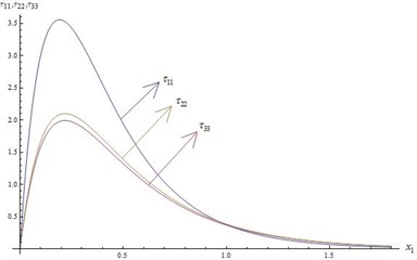
Fig. 2Distribution of Stresses for t= 0.8 and ω= 4 verses x1

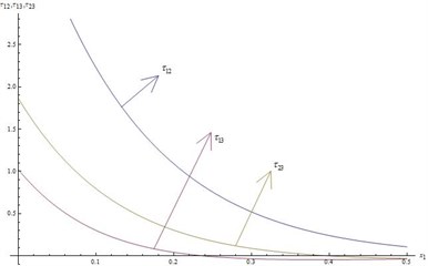
Fig. 3Distribution of Shearing Strains for t= 0.3 and ω= 3 verses x1

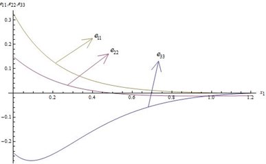
Fig. 4Distribution of Shearing Strains for t= 0.3 and ω= 3 verses x1

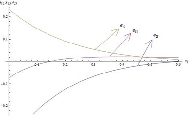
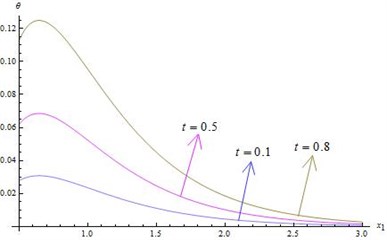
Fig. 5Distribution of temperature for ω= 2 and x2=x3= 0.5 verses x1

2) In Fig. 3 and 4 we notice the variation of dimensionless strain components for fixed values of $ω =$ 3, $r^{*} =$ 20 and $t =$ 0.6 verses space variable $x_{1}$ .

• Absolute values of strain components gradually decrease as space variable $x_{1}$ increases and finally vanish.

• The strain components $e_{11}$ , $e_{22}$ and $e_{12}$ areextensive whereas $e_{33}$ and $e_{23}$ are compressive.

• The characteristic of $e_{11}$ , $e_{22}$ and $e_{12}$ are same with respect to wave propagation.

• The non-dimensional shearing strain components $e_{13}$ is compressive within the region 0 $\leq x_{1} \leq$ 0.15 and extensive beyond $x_{1} \geq$ 0.15 and finally vanish.

3) Fig. 5 represents the variation of non-dimensional temperature $θ$ for fixed time, when $ω =$ 2, $r^{*} =$ 20 and $x_{2} = x_{3} =$ 0.5 verses $x_{1}$ .

• Temperature gradually decreases as space variable $x_{1}$ increases for all time.

• For fixed $x_{1}$ , $θ$ gradually increases as time t increases.

4) Figs. 6-9 represent the variations of stresses and strains for fixed time when $r^{*} =$ 20 and $x_{1} = x_{2} = x_{3} =$ 0.5 verses $ω$ ( $\leq$ 1).

• From these figures it is clear that $τ_{22}$ and $τ_{12}$ (normal and shearing stresses), $e_{22}$ and $e_{13}$ (normal and shearing strains) are discontinuous in the neighborhood of $ω =$ 0.6 for $t =$ 0.1, $t =$ 0.5 and $t =$ 0.8.

• $τ_{22}$ is extensive except in the region 0.58 $\leq ω \leq$ 0.64 for all $t =$ 0.1, $t =$ 0.5 and $t =$ 0.8.

• $τ_{12}$ is compressive except in the region 0.57 $\leq ω \leq$ 0.59 for all $t =$ 0.1, 0.5 and 0.8.

• From Fig. 8, it is clear that $e_{22}$ is always positive within the region 0 $\leq ω \leq$ 1 although it has a discontinuity at $ω$ 0.59.

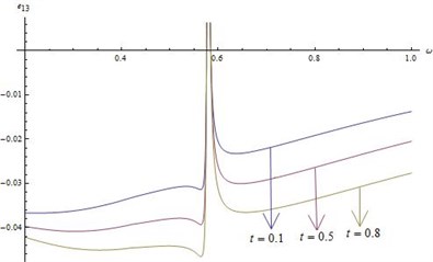
• Fig. 9 depicted that $e_{13}$ is always negative within the region 0 $\leq ω \leq$ 1 although it has a discontinuity at $ω =$ 0.59.

• $τ_{22}$ , $τ_{12}$ , $e_{22}$ and $e_{13}$ are maximum (absolute value) for $t =$ 0.8 within the region 0 $\leq ω \leq$ 1.

• Nature of discontinuities of $τ_{11}$ , $τ_{33}$ , $τ_{23}$ and $τ_{13}$ are almost same as $τ_{22}$ and $τ_{12}$ .

• The discontinuities of other strain components and $e_{11}$ , $e_{33}$ , $e_{12}$ and $e_{23}$ are also same as $e_{22}$ and $e_{13}$ .

Fig. 6Distribution of τ22 for fixed x1=x2=x3= 0.5 and r*= 20 for different values of ω

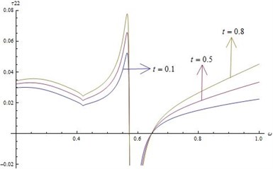
Fig. 7Distribution of τ12 for fixed x1=x2=x3= 0.5 and r*= 20 for different values of ω

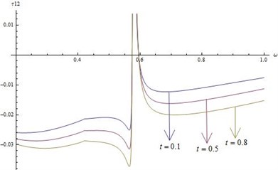
Fig. 8Distribution of e22 for fixed x1=x2=x3= 0.5 and r*= 20 for different values of ω

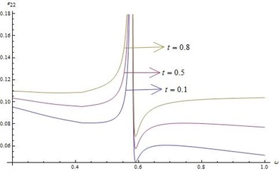
Fig. 9Distribution of e13 for fixed x1=x2=x3= 0.5 and r*= 20 for different values of ω

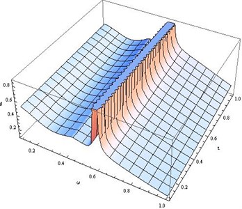
5) Figs. 10-12 depict the distribution of stresses $τ_{11}$ , $τ_{12}$ and $τ_{23}$ for 0 $< ω \leq$ 1 and time t in the fixed plane $x_{1} =$ 0.3 when $r^{*} =$ 200.

• Fig. 10 shows that normal stress $τ_{11}$ is discontinuous within 0.59 $\leq ω \leq$ 0.61 for all values of time $t$ (0 $< t <$ 0.3). Numerical values of $τ_{11}$ slowly increases with time for fixed $ω$ . On the other hand for fixed time $t$ , $τ_{11}$ changes rapidly when 0.61 $\leq ω \leq$ 1.0 for 0 $< t \leq$ 0.3.

• From Fig. 11 it is clear that shearing stress $τ_{12}$ is compressive for 0 $\leq ω \leq$ 1.0 and 0 $< t <$ 0.3 except at the point of discontinuity 0.58 $< ω <$ 0.59. The characteristic of $τ_{12}$ is same for all time when $ω$ is fixed and vice versa.

• Fig. 12 represents the distribution of the shearing stress $τ_{23}$ which is extensive for 0 $< ω \leq$ 1 and 0 $< t <$ 0.3. It can be noticed that $τ_{23}$ is discontinuous within 0.58 $< ω <$ 0.60. $τ_{23}$ gradually decreases for fixed time t when 0.2 $< ω <$ 0.57. Beyond the discontinuity region for fixed $ω$ , $τ_{23}$ steadily increases as time t increases.The numerical value of $τ_{23}$ gradually decreases for fixed time as $ω$ increases.

• The nature of $τ_{13}$ is same as $τ_{23}$ _.

• The nature of wave propagation of $τ_{22}$ and $τ_{33}$ are same as $τ_{11}$ .

Fig. 10Distribution of τ11 for fixed x1= 0.3 and different values of ω, t

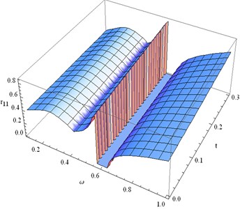
Fig. 11Distribution of τ12 for fixed x1= 0.3 and different values of ω, t

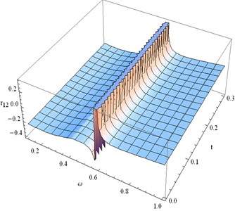
Fig. 12Distribution of τ23 for fixed x1= 0.3 and different values of ω, t

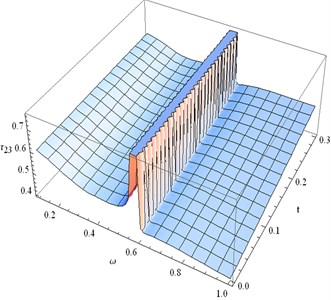
Fig. 13Distribution of e33 for fixed x1= 0.3 and different values of ω, t

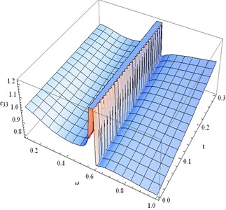
6) Figs. 13-16 represent distribution of strains $e_{33}$ , $e_{12}$ , $e_{23}$ and $e_{13}$ for $ω$ (≤ 1) and time $t$ in the fixed plane $x_{1} =$ 0.3 when $r^{*} =$ 200.

• Fig. 13 shows that the normal strain components $e_{33}$ is discontinuous for 0.58 $< ω <$ 0.60 and 0 $< t \leq$ 0.3. Also we see that $e_{33}$ gradually decreases for fixed time when 0.2 $< ω <$ 0.56. For fixed $ω$ , $e_{33}$ steadily increases as time $t$ (0 $< t \leq$ 0.3) increases.

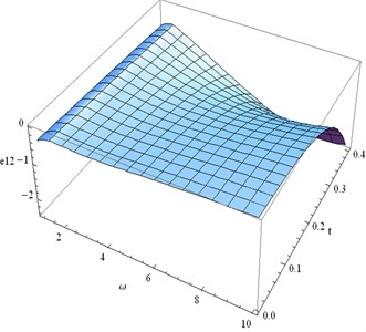
• Fig. 14 display the distribution of strain components $e_{12}$ which is discontinuous for 0.58 $< ω <$ 0.60 and 0 $< t \leq$ 0.3. For fixed time $t$ , $e_{12}$ gradually decreases within the region 0.2 < $ω$ ≤ 0.40 and then slowly increases in 0.4 $< ω \leq$ 0.58. After the location of the discontinuity, $e_{12}$ gradually increases as $ω$ increases. Nothing significant changes can be noticed for fixed $ω$ when time $t$ changes.

• Fig. 15 depicts that the strain component $e_{23}$ is discontinuous when 0.56 $< ω <$ 0.60 for all time 0 $< t \leq$ 0.3. Also we can notice that $e_{23}$ is positive like $e_{33}$ for 0 $< ω \leq$ 1 and 0 $< t \leq$ 0.3. For fixed $ω$ , $e_{23}$ increases as time t increases.

• Fig. 16 represents the distribution of strain component $e_{13}$ which is discontinuous within the region 0.58 $< ω <$ 0.60 for all time 0 $< t \leq$ 0.3.

Fig. 14Distribution of e12 for fixed x1= 0.3 and different values of ω, t

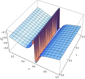
Fig. 15Distribution of e23 for fixed x1= 0.3 and different values of ω, t

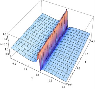
Fig. 16Distribution of e13 for fixed x1= 0.3 and different values of ω, t

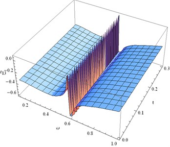
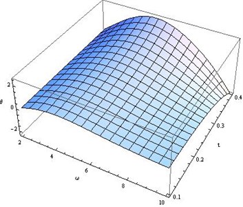
Fig. 17Distribution of θ for fixed x1=x2=x3= 0.8, r*= 200 and different values of ω, t

7) Fig. 17 displays the distribution of temperature $θ$ for different values of $ω$ and time $t$ . For fixed time, $θ$ gradually decreases for 0 $< ω <$ 0.56. Temperature is maximum for all time 0.56 $< ω <$ 0.60 and then gradually decreases. For fixed $ω$ , $θ$ slowly increases as time $t$ increases.

8) Figs. 18-20 are drawn to show the distribution of normal and shearing stresses for 0 $< ω \leq$ 10 and 0 $< t \leq$ 0.5 in the fixed plane $x_{1} =$ 0.3 when $r^{*} =$ 200.

• From Fig. 18 it is clear that significant changes occur within 3.5 $< ω <$ 7.5 and 2.5 $\leq t \leq$ 0.4. For fixed $ω$ , $τ_{11}$ gradually increases as time $t$ (0.25 $\leq t \leq$ 0.45) increases and gradually decreases for fixed time when 0 $< ω <$ 10.

• Fig. 19 shows that shearing stress $τ_{12}$ gradually increases for fixed $ω$ (2 $\leq ω \leq$ 10) when $t$ (0 $\leq t \leq$ 0.4). It can be noted that $τ_{12}$ is maximum when $ω =$ 10 and $t =$ 0.4.

• Fig. 20 depicts that for fixed time, $τ_{13}$ gradually decreases as $ω$ increases which is more prominent for $t =$ 0.4 and 0 $< ω <$ 8. After attending the minimum value $τ_{13}$ gradually increases for 8 $< ω <$ 10 and 0.35 $\leq t \leq$ 0.4.

• Nature of $τ_{22}$ and $τ_{33}$ are almost same as $τ_{11}$ .

9) Figs. 21-24 show the distribution of strains in the fixed plane $x_{1} =$ 0.3 when $r^{*} =$ 200 for different values of $ω$ and $t$ .

Fig. 18Distribution of τ11 for fixed x1= 0.3 and different values of ω, t

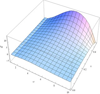
Fig. 19Distribution of τ12 for fixed x1= 0.3 and different values of ω, t

Fig. 20Distribution of τ13 for fixed x1= 0.3 and different values of ω, t

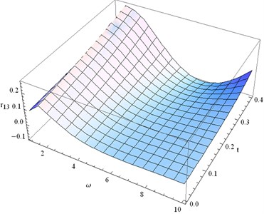
Fig. 21Distribution of e11 for fixed x1= 0.3 and different values of ω, t

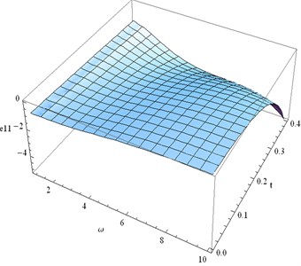
Fig. 22Distribution of e33 for fixed x1= 0.3 and different values of ω, t

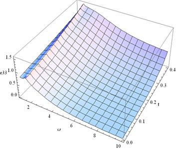
Fig. 23Distribution of e12 for fixed x1= 0.3 and different values of ω, t

• Figs. 21 and 22 represent the distributions of the normal strain components. We notice that $e_{11}$ is negative for all 0 $< ω \leq$ 10 and 0 $< t <$ 0.4 while $e_{33}$ is positive. Numerical value of $e_{11}$ gradually tends to zero when $ω$ tends to 10 and $t$ tends to 0.4. On the other hand $e_{33}$ becomes zero when $ω =$ 10 and $t =$ 0.4.

• Fig. 23 depicts the distribution of the shearing strain $e_{12}$ . Characteristic of $e_{12}$ is almost same as $e_{11}$ .

• Fig. 24 shows that for fixed $ω$ , numerical value of $e_{13}$ gradually increasing as time $t$ increases. For fixed time $t$ , $e_{13}$ slowly increases as $ω$ increases.

10) Fig. 25 displays the temperature distribution for 2 $\leq ω \leq$ 10 and 0 $< t \leq$ 0.4. Temperature attains its maximum value when $ω =$ 6 and $t =$ 0.4. Temperature increases slowly when 2 $\leq ω \leq$ 6 and 0.15 $\leq t \leq$ 0.4 then gradually decreases.

Fig. 24Distribution of e13 for fixed x1= 0.3 and different values of ω, t

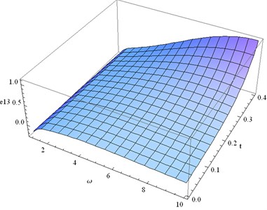
Fig. 25Distribution of θ for fixed x1=x2=x3= 0.5, r*= 200 and different values of ω, t

8. Applications and uncertainties

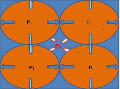
Subsurface rocks are generally filled with cracks and pore spaces saturated with one or more fluids such as oils, water and gasses which can influence the mechanical behavior of rocks. Thermal expansion of existing fluids due to thermo-poroelastic stress field causes gradual increase of fluid pressure in the intergranular spaces. If the fluid pressure (Pf) exceeds lithostatic pressure (Pl) by more than the tensile strength of the rock (usually small) the rock is likely to burst due to hydraulic fracturing and in the process fluid will migrate along the cracks developed (Fig. 26). The migration of oil and gas can be accentuated through these cracks into suitable structural traps producing voluminous oil and gas field in the rocks.

Fig. 26Schematic diagram showing developments of hydraulic fracturing in matrix of rocks. Pl = Lithostatic Pressure and Pf = Fluid Pressure

$Schematic diagram showing developments of hydraulic fracturing in matrix of rocks. Pl = Lithostatic Pressure and Pf = Fluid Pressure$

According to linear elastic fracturing model three distinct modes of fracturing can be generated depending on the three different types of loading (Irwin [37]). In Mode-I, the tensile forces are applied normal to the crack plane so that the crack planes are pulled apart enabling the crack more and more open (Fig. 27(a)). In Mode-II, the cracked body is loaded by shear forces acting parallel to the crack surfaces, which slide over each other in the applied direction (Fig. 27(b)). In Mode-III the cracked body is also loaded by shear forces but parallel to the crack front and the fracture planes slide over each other out of the plane direction (Fig. 27(c)). In case of Mode-III, a large angle of sliding of rock blocks or plates may indicate a relative rotation of plates, resulting a significant amount of evolution of energy. A distinct discontinuity in the thermo-elastic curves shown whenever the $ω$ value of considerable amount rotated clockwise or anticlockwise (Fig. 27(c)) possibly indicates movements of plate with significant release of energy.

Fig. 27Three types of fractures modes (Anderson [45])

$Three types of fractures modes (Anderson [45])$

a) Mode I. Opening mode

$Three types of fractures modes (Anderson [45])$

b) Mode II. Sliding mode

$Three types of fractures modes (Anderson [45])$

c) Mode III. Tearing mode

Thus, lithospheric plates, though rigid, must certainly undergo small elastic strains showing time-dependent deformations or creep, even in very low levels of differential stress. Thus, the time-dependent heat sources appear to produce significant stresses in the lithospheric plates resulting intraplate tectonics (Turcotte [38]). It has been appreciated that the midplate swells are the results of thermal perturbations of intra-plate hot spot plumes as the plates move over the deep mantle thermal anomaly (Wilson [39]). The major uncertainties appear to be the variations of minimum depth of reheating with corresponding assumptions of surface heat flow anomalies. These constraints may result conservative estimation of the magnitude of the conductive heating in the elastic lithosphere. But the magnitudes of the calculated temperature perturbations and the related thermo-elastic stress accumulation are significant as shown in the mathematical calculations. Shallow reheating depths and larger heat flow anomalies obviously increase the temperature perturbations within the lithosphere. The effect of higher heat flow may be partially compensated in case of deeper reheating depths. Thus, the application of thermo-elastic stress analyses is more suitable for relatively thinner and homogeneous younger oceanic lithosphere. The geographical distributions of thermo-elastic stresses and their orientations are highly significant for the tectonic evolution of the plates and can be measured by earthquake focal mechanism.

Several thermo-elastic stress models applied to hotspot reheating show considerably higher deviatoric stresses for both slow and fast moving plates. Although the thermal stress fields orientations appear to be complex in pattern a horizontal extension at shallow depths and horizontal compressions near the bottom of the elastic lithosphere have been appreciated. The thermal stress configuration depends on the absolute plate velocity. Thus, fast moving plates do not get enough time for conducting heat into the poorly conducting elastic plates and as a result a large deviatoric thermal stress generates far downstream hotspot chain. While a slow moving plate appears to get enough time to interact with the underlying hotspot and creates a more circular and larger thermal field closer to the hotspot location. Obviously, the area of the thermal stress perturbation is much larger for a fast moving plate and has little or no effect to the earthquakes related to hotspots e.g., most of the earthquakes in Howaii Island (Zhu and Wiens [33], Koyanagi et al. [40], Ando [41]). However, in case of slow moving plates the effect of radial thermal stresses closer to the hotspot swells have convincingly shown direct relation to the shallow focus earthquakes (Stewart and Helmberger [42], Nishenko and Kafka [43], Bergman [44]). The focal depths of these earthquakes often mismatch to the predicted depths derived from varied thermal stress models. Thermoelastic stress structures studied in different hotspot swells show an extension perpendicular to the swell axis in shallow depths. The passage of magma through the upper part of the lithosphere is thought to be guided by this extensional stress direction. In case of moderate to slow movements of plates this tensional stresses appear to accumulate considerably long distances downstream from the hotspot location. Volcanic rejuvenation along island arcs may thus result long after the passage of hotspots. During this long time period any kind of changes in the direction of plates or rotation of plate motion, as discussed, may explain the significant changes in the initial hotspot chains as noted a 65 degrees change in direction of hotspot chain in Hawaii Island. To confirm the pattern of maximum thermal stress orientations more thermal stress modeling are appreciated near hotspots in association with earthquakes. Thus, mathematical calculations related to thermo-elastic behavior of isotropic plates subjected to temperature perturbations and various boundary conditions may show certain pathways to solve many queries about the plate-tectonic processes and associated heat sources.

9. Concluding remarks

In this paper we derive the exact analytical expression for non-dimensional stresses, strains and temperature of a homogeneous anisotropic half space medium of most general symmetry (triclinic) of thermoelasticity without energy dissipation (G-N model II) is considered. The time dependent heat source is applied at the boundary of the half space. We observe the following conclusions based on the above analysis.

1) The time dependent heat source has a significant effect on the physical quantities.

2) The maximum changes occur near the heated region.

3) From Figs. 1-5, it is clear that the numerical values of physical quantities converge to zero as $x_{1}$ increases.

4) It is clear from Figs. 6-17 that the changes in the values of $ω$ causes discontinuities of the physical quantities in the neighborhood of 0.56 $< ω <$ 0.62.

5) Figs. 18-25 depicts that the changes in the values of time $t$ and $ω$ ( $>$ 1) cause significant changes in all the physical quantities.

References

Biot M. A. Thermoelasticity and irreversible thermodynamics. Journal of Applied Physics, Vol. 27, 1956, p. 240-253.

Publisher
Lord H. W., Shulman Y. A generalized dynamical theory of thermoelasticity. Journal of Mechanics and Physics of Solids, Vol. 15, 1967, p. 299-309.

Publisher
Dhaliwal R. S., Sherief H. H. Generalized thermoelasticity for anisotropic media. Quarterly of Applied Mathematics, Vol. 33, 1980, p. 1-8.

Publisher
Ignaczak J. Uniqueness in generalized thermoelasticity. Journal of Thermal Stresses, Vol. 2, 1979, p. 171-175.

Publisher
Ignaczak J. A note on uniqueness in thermoelasticity with one relaxation time. Journal of Thermal Stresses, Vol. 5, 1982, p. 257-263.

Publisher
Green A. E., Lindsay K. A. Thermoelasticity. Journal of Elasticity, Vol. 2, 1972, p. 1-7.

Publisher
Green A. E., Naghdi P. M. A re-examination of the basic postulate of thermomechanics. Proceedings of Royal Society of London, Vol. 432, 1991, p. 171-194.

Publisher
Green A. E., Naghdi P. M. On undamped heat waves in an elastic solid. Journal of Thermal Stresses, Vol. 15, 1992, p. 253-264.

Publisher
Green A. E., Naghdi P. M. Thermoelasticity without energy dissipation. Journal of Elasticity, Vol. 31, 1993, p. 189-208.

Publisher
Roychoudhuri S. K., Bandyopadhyay N. Thermoelastic wave propagation in a rotating elastic medium without energy dissipation. International Journal of Mathematics and Mathematical Sciences, Vol. 1, 2004, p. 99-107.

Publisher
Roychoudhuri S. K., Dutta P. S. Thermoelastic interaction without energy dissipation in an infinite solid with distributed periodically varying heat sources. International Journal of Solids and Structures, Vol. 42, 2005, p. 4192-4203.

Publisher
Sharma J. N., Chouhan R. S. On the problem of body forces and heat sources in thermoelasticity without energy dissipation. Indian Journal of Pure and Applied Mathematics, Vol. 30, 1999, p. 595-610.

Search CrossRef
Chandrasekharaiah D. S., Srinath K. S. Thermoelastic plane waves without energy dissipation in a rotating body. Mechanics Research Communications, Vol. 24, 2000, p. 551-560.

Publisher
Sarkar N., Lahiri A. A three dimensional thermoelastic problem for a half Space without energy dissipation. International Journal of Engineering Science, Vol. 51, 2012, p. 310-325.

Publisher
Bachher M., Sarkar N., Lahiri A. State-space approach to 3D generalized thermoviscoelasticity under Green and Naghdi theory II. Mathematical Models in Engineering, Vol. 1, 2015, p. 111-124.

Search CrossRef
Othman M. I. A., Lotfy K. H., Farouk R. K. Transient disturbance in a half-space using generalized magneto-thermoelasticity with internal heat source. Acta Physica Polonica A, Vol. 116, 2009, p. 185-192.

Publisher
Pal P. K., Acharya D. Effects of inhomogeneity on the surface waves in anisotropic media. Sadhana, Vol. 23, 1998, p. 247-258.

Publisher
Pal P. C., et al. Wave propagation in an inhomogeneous anosotropic generalized thermoelastic solid. Journal of Thermal Stresses, Vol. 37, 2014, p. 817-831.

Publisher
Achenbach J. D. Wave Propagation in Elastic Solids. North Holland, New York, 1976.

Search CrossRef
Nayfeh A. H. Wave Propagation in Layered Anisotropic Media with Application to Composites. Elsevier, Amsterdam, 1995.

Search CrossRef
Pal A. K., Chattopadhyay A. The reflection phenomena of plane waves at a free boundary in a pre-stressed elastic half-space. Journal of the Acoustical Society of America, Vol. 76, 1984, p. 924-925.

Publisher
Chattopadhyay A., Rogerson G. A. Wave reflection in slightly compressible, finitely deformed elastic media. Archive of Applied Mechanics, Vol. 71, 2001, p. 307-316.

Publisher
Sharma M. D. 3-D wave propagation in a general anisotropic poroelastic medium: reflection and transmission at an interface with fluid. Geophysical Journal International, Vol. 157, 2004, p. 947-958.

Publisher
Chattopadhyay A., Kumari P., Sharma V. K. Reflection and refraction at the interface between distinct generally anisotropic half spaces for three-dimensional plane quasi-P waves. Journal of Vibration and Control, Vol. 21, 2015, p. 493-508.

Publisher
Mensch T., Rasolofosaon P. Elastic-wave velocities in anisotropic media of arbitrary symmetry generalization of Thomson’s parameters ε, δ and γ. Geophysical Journal International, Vol. 128, 1997, p. 43-64.

Publisher
Abbas I. A., Othman M. I. A. Generalized thermoelastic interaction in a fiber-reinforced anisotropic half-space under hydrostatic initial stress. Journal of Vibration and Control, Vol. 18, 2011, p. 175-182.

Publisher
Verma K. L. Thermoelastic waves in anisotropic plates using normal mode expansion method with thermal relaxation time. World Academy of Science, Engineering and Technology, Vol. 2, 2008, p. 19-26.

Search CrossRef
Zhou B., Greenhalgh S. On the computation of elastic wave group velocities for a general anisotropic medium. Journal of Geophysics and Engineering, Vol. 1, 2004, p. 205-215.

Publisher
Grechka V. Shear-wave group-velocity surfaces in low-symmetry anisotropic media. Geophysics, Vol. 80, 2015, p. 1-7.

Publisher
Vernik L., Liu X. Velocity anisotropy in shale: a petrophysical study. Geophysics, Vol. 62, 1997, p. 521-532.

Publisher
Kumar R., Gupta V. Plane wave propagation in an anisotropic thermoelastic medium with fractional order derivative and void. Journal of Thermoelasticity, Vol. 1, 2013, p. 21-34.

Search CrossRef
Othman M. I. A., Atwa S. Y., Elwan A. W. Two and three dimensions of generalized thermoelastic medium without energy dissipation under the effect of rotation. Applied Mathematics, Vol. 6, 2015, p. 793-805.

Publisher
Zhu A., Wiens D. A. Thermoelastic stress in oceanic lithosphere due to hotspot reheating. Journal of Geophysical Research, Vol. 96, 1991, p. 18323-18334.

Publisher
Othman M. I. A., Song Y. Effect of rotation on plane waves of generalized electro-magneto-thermoviscoelasticity with two relaxation times. Applied Mathematical Modelling, Vol. 32, 2008, p. 811-825.

Publisher
Santra S., Das N. C., Kumar R., Lahiri A. Three dimensional fractional order generalized thermoelastic problem under effect of rotation in a half space. Journal of Thermal Stresses, Vol. 38, 2015, p. 309-324.

Publisher
Lahiri A., Das N. C., Sarkar S., Das M. Matrix method of solution of coupled differential equations and its application to generalized thermoelasticity. Bulletin of the Calcutta Mathematical Society, Vol. 101, 2009, p. 571-590.

Search CrossRef
Irwin G. R. Analysis of stresses and strains near the end of a crack traversing a plate. Journal of Applied Mechanics, Vol. 24, 1957, p. 361-364.

Publisher
Turcotte D. L. Are transform faults thermal contraction cracks? Journal of Geophysical Research, Vol. 79, 1974, p. 2573-2577.

Publisher
Wilson J. T. A possible origin of the Hawaiian Islands. Canadian Journal of Physics, Vol. 41, 1963, p. 863-870.

Publisher
Koyanagi R. Y., Endo E. T., Ebisu J. S. Reawakening of Mauna Loa volcano, Hawaii: a preliminary evaluation of seismic evidence. Geophysical Research Letters, Vol. 2, 1975, p. 405-408.

Publisher
Ando M. The Hawaiian earthquake of November 29, 1975: Low dip angle faulting due to forceful injection of magma. Journal of Geophysical Research, Vol. 84, 1979, p. 7616-7626.

Publisher
Stewart G. S., Helmberger D. V. The Bermuda earthquake of March 24, 1978; a significant oceanic intraplate event. Journal of Geophysical Research, Vol. 86, 1981, p. 7020-7036.

Publisher
Nishenko S. P., Kafka A. L. Earthquake focal mechanisms and the intraplate setting of the Bermuda Rise. Journal of Geophysical Research, Vol. 87, 1982, p. 3929-3941.

Publisher
Bergman E. A. Intraplate earthquakes and the state of stress in oceanic lithosphere. Tectonophysics, Vol. 132, 1986, p. 1-35.

Publisher
Anderson T. L. Fracture Mechanics: Fundamentals and Applications. Taylor and Francis, Boca Raton, FL, 2005.

Publisher

Cited by

Influence of distinct type of imperfect interfaces on reflection and transmission phenomena of triclinic thermoelastic structure

Pooja Singh | Abhishek Kumar Singh | Amares Chattopadhyay

(2021)

One-dimensional nonlinear vibration analysis and coupled thermoelasticity based on Green-Naghdi model

Mohammad Hosein Nejabat Meimandi | Ali Reza Fotuhi | Mohammad Reza Fazel

(2019)

About this article

Received

26 August 2016

Accepted

27 October 2016

Published

31 December 2016

DOI

https://doi.org/10.21595/mme.2016.17621

Keywords

anisotropic solid

Green-Naghdi model II

normal mode analysis

eigenvalue approach

lithostatic pressure and lithospheric plates

This is an open access article distributed under the Creative Commons Attribution License, which permits unrestricted use, distribution, and reproduction in any medium, provided the original work is properly cited.

Previous article in issue Previous Next article in issue Next

Research article

2023 12 23

Plane waves in an isotropic thermoelastic diffusive material using strain gradient theory

Baljeet Singh, Himanshu Singla

Research article

2023 06 26

Influence of the fractional-order strain on an infinite material with a spherical cavity under Green-Naghdi hyperbolic two-temperature thermoelasticity theory

Hamdy M. Youssef, Abdulrahman A. Alghamdi

Research article

2022 06 30

The vibration of a thermoelastic nanobeam due to thermo-electrical effect of graphene nano-strip under Green-Naghdi type-II model

Hamdy M. Youssef, Abdullah A. Al Thobaiti

Research article

2019 09 30

Thermal shock behaviour on generalized thermoelastic semi-infinite medium with moving heat source under Green Naghdi-III model

Biswajit Singh, Smita Pal (Sarkar)

S. Chakraborty, S. C. Mandal, A. K. Das, N. Sarkar, and A. Lahiri, “Plane wave propagation in a 3D anisotropic half-space under Green-Naghdi theory II,” Mathematical Models in Engineering, Vol. 2, No. 2, pp. 114–134, Dec. 2016, https://doi.org/10.21595/mme.2016.17621

Copy Extrica

Copied to clipboard!

TY  - JOUR
DO  - 10.21595/mme.2016.17621
UR  - https://doi.org/10.21595/mme.2016.17621
TI  - Plane wave propagation in a 3D anisotropic half-space under Green-Naghdi theory II
T2  - Mathematical Models in Engineering
AU  - Sarkar, N.
AU  - Chakraborty, S.
AU  - Mandal, S. C.
AU  - Das, A. K.
AU  - Lahiri, A.
PY  - 2016
DA  - 2016/12/31
PB  - JVE International Ltd.
SP  - 114-134
IS  - 2
VL  - 2
SN  - 2351-5279
SN  - 2424-4627
ER  - 

Copy Ris

Copied to clipboard!

@article{Sarkar_2016,
	doi = {10.21595/mme.2016.17621},
	url = {https://doi.org/10.21595/mme.2016.17621},
	year = 2016,
	month = {dec},
	publisher = {{JVE} International Ltd.},
	volume = {2},
	number = {2},
	pages = {114--134},
	author = {N. Sarkar and S. Chakraborty and S. C. Mandal and A. K. Das and A. Lahiri},
	title = {Plane wave propagation in a 3D anisotropic half-space under Green-Naghdi theory {II}},
	journal = {Mathematical Models in Engineering}
}

Copy Bibtex

Copied to clipboard!

[1]N. Sarkar, S. Chakraborty, S. C. Mandal, A. K. Das, and A. Lahiri, “Plane wave propagation in a 3D anisotropic half-space under Green-Naghdi theory II,” Mathematical Models in Engineering, vol. 2, no. 2, pp. 114–134, Dec. 2016, doi: 10.21595/mme.2016.17621.

Copy IEEE

Copied to clipboard!

Sarkar, N., S. Chakraborty, S. C. Mandal, A. K. Das, and A. Lahiri. “Plane Wave Propagation in a 3D Anisotropic Half-Space under Green-Naghdi Theory II.” Mathematical Models in Engineering 2, no. 2 (December 31, 2016): 114–34. https://doi.org/10.21595/mme.2016.17621.

Copy Chicago

Copied to clipboard!

Plane wave propagation in a 3D anisotropic half-space under Green-Naghdi theory II

Abstract

1. Introduction

2. Basic equations

3. Formulation of the problem

4. Normal mode analysis: Formulation of vector–matrix differential equation

5. Solution of the vector-matrix differential equation: Eigenvalue approach

6. Boundary conditions

7. Numerical example and discussion

8. Applications and uncertainties

9. Concluding remarks

References

Cited by

About this article

Related Articles