Abstract
A dynamical analysis of a Mathieu-van der Pol-Duffing nonlinear system with fractional-order derivative under combined parametric and forcing excitation is studied in this paper. The approximate analytical solution is researched for 1/2 sub harmonic resonance coupled with primary parametric resonance based on the improved averaging approach. The steady-state periodic solution including its stability condition is established. The equivalent linear stiffness coefficient (ELDC) and equivalent linear damping coefficient (ELSC) for this nonlinear fractional-order oscillator are defined. Then, the numerical simulations are presented in three typical cases by iterative algorithms. The time history, phase portrait, FFT spectrum and Poincare maps are shown to explain the system response. Some different responses, such as quasi-periodic, multi-periodic and single periodic behaviors are observed and investigated. The results of comparisons between the numerical solutions and the approximate analytical solutions in three typical cases show the correctness of the analytical solutions. The influences of the fractional-order parameters on the system dynamical response are researched based on the ELDC and ELSC. Through analysis, it could be found that the increase of the fractional-order coefficient would result in the rightward and downward movements of the amplitude-frequency curves. The increase of the fractional-order coefficient will also move the bifurcation point rightwards and will make the existing range of steady-state solution larger. It could also be found that the ELSC will become larger and ELDC smaller when the fractional order is closer to zero, so that the decrease of the fractional order would make the response amplitude larger. At last, the detailed conclusions are summarized, which is beneficial to design and control this kind of fractional-order nonlinear system.
1. Introduction
With the development of modern computation technology in recent years, the fractional calculus has caused wide concerns in many fields, especially in mechanical, civil, biological and other engineering fields. The fundamental characteristics of fractional calculus are studied, and great progress has been made in the basic theory[1-4]. For example, Petras [1-2] studied the modeling, analysis and simulation of the fractional-order nonlinear systems, and they also focused on the modeling and control of the fractional-order systems. Caputo et al. [3] proposed a new definition of the fractional derivative. Yang et al. [4] investigated the local fractional integral transforms and the applications problem, etc.
At present, the applications of the fractional calculus in engineering fields have been attracted much attention. Many engineering problems can be described by the fractional calculus equations to simulate some dynamical systems accurately. So, the fractional calculus on the dynamical system was important and interesting, which had been investigated by many researchers in some relevant fields [5, 6]. For example, Yang et al. [7] analyzed the response of a fractional-order Duffing system by the harmonic balance method, and concluded that the fractional-order damping could change the number of the steady stable states. Wang et al. [8] investigated the dynamical characteristics of a linear oscillator with fractional-order derivative under forcing excitation, and found that the system solution had two parts in the fractional-order linear oscillator based on the theory of the stability switches. Shen et al. [9, 10] investigated several fractional-order oscillators by the averaging method, and proposed the fractional-order derivative that had both the function of damping and the function of stiffness. Many mathematical theories of the fractional calculus were researched by Li et al. [11, 12]. They also compared the differences and connections between three typical definitions of fractional-order derivatives, and presented some characteristics of the Caputo fractional calculus. Chen et al. [13] studied the dynamical response of the fractional-order stochastic oscillator based on the stochastic averaging approach, and they mainly analyzed the influences of the fractional-order derivative on the dynamics and the control of the stochastic system. Leung et al. [14] raised the residue harmonic balance approach to solve the fractional-order van der Pol (VDP) system and the higher-order approximate solution could be deduced according to this method. You et al. [15] studied the optimal control of a fractional-order vehicle suspension system, and the viscoelastic characteristics of the vehicle suspension system were investigated. Shen et al. [16] studied the fractional-order PID controller on a non-smooth oscillator and found the fractional-order PID controller was better than the traditional PID controller. Wang et al. [17] investigated the chaos behavior of the fractional-order Lorenz systems by the active feedback approach. Then the fractional order of 0.98 was implemented and the result demonstrated the validity of this method. Yang et al. [18, 19] studied several fractional-order operators in the sense of Caputo definition, and discussed their characteristics based on the Laplace transform and Fourier transform. Those results were very efficient and helpful to investigate some complex phenomenon. Li et al. [20] investigated the stochastic bifurcations of Duffing-VDP system under colored noise by the stochastic averaging method, and found that the change of fractional order, noise intensity and correlation time would lead to bifurcation of this system. Niu et al. [21] studied the Duffing oscillator with delayed fractional-order PID control based on the KBM asymptotic method, and analyzed the influences of time delay. Giresse et al. [22] studied the synchronization of chaotic Mathieu-VDP and chaotic Duffing-VDP systems with the fractional-order derivative, and found fractional-order derivative would lead to faster synchronization than the integer-order derivative.
There are many nonlinear dynamics phenomena in engineering fields, such as non-smoothness, large deformation, backlash, and parametric excitation, etc., which will deteriorate the performance of engineering system [23, 24]. For example, Li et al. [25-26] found the bursting phenomenon in a mechanical system and analyzed the slow-fast effect. Belhaq et al. [27] analyzed the resonances of VDP-Mathieu-Duffing oscillator in the frequency-locking area of 2:1 and 1:1, and found that the fast harmonic excitation could change the spring behavior. Based on the authors’ knowledge, the published papers were mainly focused on the dynamical responses of the fractional-order system with forcing excitation and the integer-order nonlinear system. A few researchers studied the fractional-order complex nonlinear system. For example, Wen et al. [28, 29] investigated the dynamical characteristics of Mathieu-Duffing oscillator with the fractional-order delayed feedback, and found that the fractional-order delayed feedback had the characteristics of both delayed velocity feedback and displacement feedback. Xu et al. [30] analyzed the dynamical responses of fractional-order Duffing-Rayleigh oscillator with the Gauss white noise excitation. But the dynamical analysis of the complex fractional-order nonlinear system with combined parametric and forcing excitation hardly has been investigated.
In this paper, the dynamical responses of Mathieu-van der Pol-Duffing nonlinear system with the fractional-order derivative for 1/2 subharmonics resonance coupled with the primary parametric resonance are studied. The paper is arranged as follows: In Section 2, the approximate analytical solution of the fractional-order Mathieu-van der Pol-Duffing nonlinear system is obtained. Then the ELDC and ELSC are also defined in this section. In Section 3, the amplitude-frequency equation and the stability conditions of the steady-state nonzero periodic solution are presented. Then in Section 4 the numerical solutions in three typical cases are obtained. The comparisons between the analytical results and the numerical solutions in three cases are presented to prove the correctness of the approximate analytical solution. The effects of the fractional-order parameters are studied in Section 5. At last, the detailed conclusions are summarized and analyzed.
2. First-order approximate analytical solution
The considered fractional-order nonlinear system with 1/2 subharmonics resonance coupled with primary parametric resonance is:
where , , , , , and are the system mass, linear stiffness coefficient, nonlinear damping coefficient, nonlinear stiffness coefficient, forcing excitation coefficient, forcing excitation frequency and the periodic time-varying stiffing coefficient respectively. is the -order derivative of to with the fractional coefficient () and fractional order (). Here the Caputo definition is used below:
where is the Gamma function which satisfies .
The following transformations are used:
Eq. (1) becomes:
Here, we focus on the 1/2 sub harmonic resonance coupled with the primary parametric resonance. It means the parametric frequency is close to the natural frequency and the forcing excitation frequency is close to the double of the parametric frequency, i.e. , . The formula is introduced to denote the approximate degree, where is the detuning factor, so that Eq. (4) becomes:
Supposing the solution of Eq. (5) is:
where . Based on the improved averaging approach [9, 10], we could integrate the right-hand part of Eq. (5) within the time interval [0, ] and then average it. The approximate solution of amplitude and phase are:
where:
When Eq. (7) is expanded, it will yield:
The first part of Eq. (8a) and Eq. (8b) are the periodic function with . Integrating the first part of Eq. (8), one could get:
The second part of Eq. (8a) and Eq. (8b) are the aperiodic functions, and the time terminal is selected as :
Considering Eq. (2), one can obtain:
Supposing , , and when they are substituted into Eq. (11), it becomes:
Two important formulae in Refs [9-10] are introduced:
In Eq. (12), defining the first part as and the second part as , integrating it by parts respectively and considering Eq. (13), one can get:
Similarly, one can find the integral of the second part in Eq. (12) approach 0 when , so that:
When the same method is used, it will yield:
Combining Eq. (9) and Eq. (15), one can obtain:
When the original parameters are substituted into Eq. (16), it will yield:
where:
are defined as the equivalent linear damping coefficient (ELDC) and the equivalent linear stiffness coefficient (ELSC) respectively.
Based on Eq. (17) and Eq. (18), it could be found that the fractional coefficient and the fractional order are all significant in system dynamics. The fractional coefficient is linear with the ELDC and ELSC in this system. The fractional order affects this system dynamical response with the ELDC and ELSC in the form of trigonometric function. When and , the fractional-order derivative will possess both the function of stiffness and the function of damping simultaneously.
3. Steady-state periodic solutions and stability conditions
Letting and , Eq. (17) becomes:
When is eliminated from Eq. (19), the amplitude-frequency equation is:
That is:
Letting , , and when they are substituted into Eq. (17), it becomes:
The Jacobian matrix for Eq. (21) is:
The Jacobian matrix of the nonzero periodic solution is:
Letting:
and using Eq. (19), the characteristic equation can be get as follows:
From the analysis of Eq. (22), it can be found that the stability conditions for the nonzero periodic solution are:
According to Eq. (20b), one could get the following results.
When , Eq. (20b) has the zero solution and one nonzero periodic solution as follows:
When:
and:
Eq. (20b) has the zero solution and two nonzero periodic solutions as follows:
According to the stability conditions of Eq. (23), it can be found that the nonzero solution given by Eq. (24) is stable and there is only one nonzero solution for Eq. (1) at this moment. When Eq. (1) has two nonzero solutions, one nonzero solution given in Eq. (25a) is stable and the other one given in Eq. (25b) is unstable.
4. Numerical simulation
Numerical simulation solutions of Eq. (1) are presented in the following part. The numerical iteration methods introduced in [1-3] are adopted and the numerical formula is:
where is the fractional binomial coefficient which satisfies the iterative relationship of Eq. (27), is the time sample points and is the sample step.
Based on Eq. (26) and Eq. (27), the numerical iterative algorithm of Eq. (1) could be obtained:
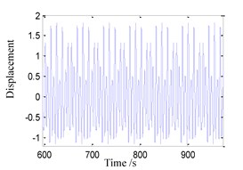
where is the displacement, is the velocity, and is the fractional-order derivative. Here the sample step is selected as 0.001. The temporary response is omitted, and the maximum steady amplitude of the posterior steady-state response is adopted. Numerical results and subsequent analysis of Eq. (1) are presented in three typical topology cases.
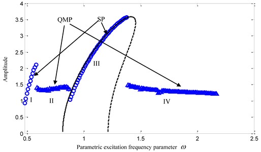
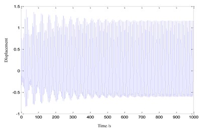
The system parameters of the first illustrative example are selected as: , , , , , , and . The numerical results are shown in Fig. 1. As the frequency is swept forward, the amplitude-frequency curve based on the numerical iterative algorithm is shown in Fig. 1 by small triangles and circles. From the observation of Fig. 1, it can be found that in the amplitude-frequency curve there are three sudden change points and four different response regions. The following parts will simulate the dynamical motions in different regions. In order to analyze the system motion, the time history figure only shows a partial steady state process in Figs. 2-7.
Fig. 1Amplitude-frequency curves: (m=1, K1=1, α1=0.1, α2=0.1, B=0.4, K2=0.1, p=0.5, F=0.5)
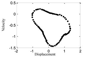
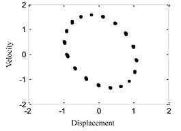
(1) When 0.55, the time history, phase portrait, FFT spectrum and Poincare maps are as shown in Fig. 2 respectively. It can be found that there is only one main frequency in the FFT spectrum of Fig. 2(c), and there is only one point in Poincare maps of Fig. 2(d), so that the system response is simple single-periodic motion in this case.
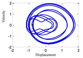
(2) When 0.75, the time history, phase portrait, FFT spectrum and Poincare maps are shown in Fig. 3 respectively. It can be found that there are three irreducible frequency components in the FFT spectrum of Fig. 3(c), and there is a closed loop in Poincare maps of Fig. 3(d), so that the system response is quasi-periodic motion in this case.
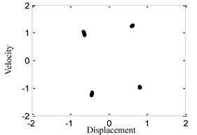
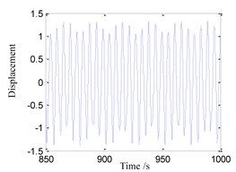
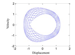
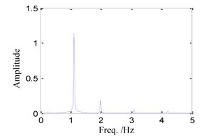
(3) When 0.8, the time history, phase portrait, FFT spectrum and Poincare maps are shown in Fig. 4 respectively. There are several frequency components in the FFT spectrum of Fig. 4(c) and several points in Poincare maps of Fig. 4(d). It can be found that the system response is multi-periodic motion in this case which is in the midst of quasi-periodic motion and single-periodic motion.
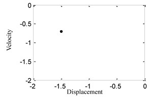
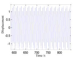
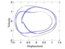
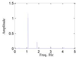
(4) When 1.0, the time history, phase portrait, FFT spectrum and Poincare maps are shown in Fig. 5 respectively. The motion characteristics are similar to those shown in Fig. 2, so that the system response also is single-periodic motion in this case.
(5) When 1.5, the time history, phase portrait, FFT spectrum and Poincare maps are shown in Fig. 6 respectively. When 1.55, the time history, phase portrait, FFT spectrum and Poincare maps are shown in Fig. 7 respectively. It can be found that the motion characteristics are similar to those shown in Fig. 4, so that the system responses are all multi-periodic motion in those cases.
Fig. 2System response for ω= 0.55
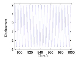
a) Time history
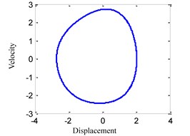
b) Phase portrait
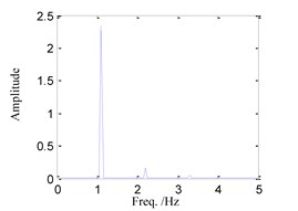
c) FFT spectrum
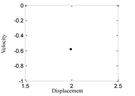
d) Poincare maps
Fig. 3System response for ω= 0.75
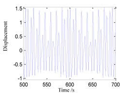
a) Time history
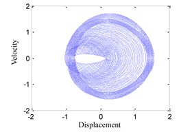
b) Phase portrait
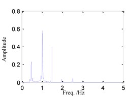
c) FFT spectrum
d) Poincare maps
Fig. 4System response for ω= 0.8
a) Time history
b) Phase portrait
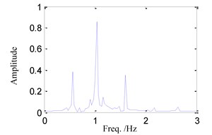
c) FFT spectrum
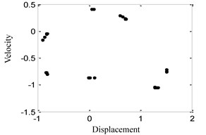
d) Poincare maps
Fig. 5System response for ω= 1.0
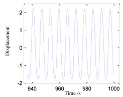
a) Time history
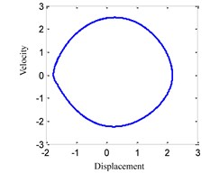
b) Phase portrait
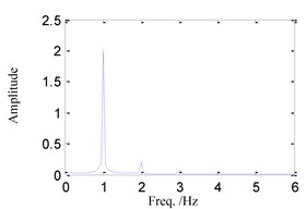
c) FFT spectrum
d) Poincare maps
We can find that there are quasi-periodic behaviors and multi-periodic behaviors (QMP) in Region II and IV denoted by small triangles, and single-periodic behaviors (SP) in Region I and III denoted by small circles in Fig. 1. With the frequency increase, the SP, QMP, SP and then QMP responses will take place in this system gradually. The SP response in Region I is the super harmonic resonance, and the SP response in Region III is the primary resonance.
The numerical results of the other two cases are shown in Fig. 8 and Fig. 9. The amplitude-frequency curves of the approximate analytical solution of Eq. (20) in three typical cases are also shown in Fig. 1, Fig. 8 and Fig. 9 respectively, where the solid line shows the stable solution and the dash line shows the unstable one. From the observation of Fig. 1, Fig. 8 and Fig. 9, one can find that the analytical solutions are all in a good agreement with the numerical ones at the regions 1 in three topology cases. Here 1/2 sub harmonic resonance coupled with the primary parametric resonance is focused, so that the correctness and accuracy of the analytical solutions can be verified. Furthermore, we also find that the approximate analytical solution does not agree very well with the numerical one near the bifurcation points on the both sides in Region III of Fig. 1. In order to analyze the error reason, two points 0.87 and 0.875 near the bifurcation points are selected to simulate time histories in Fig. 10(b) and Fig. 10(a) respectively. From the comparison of Fig. 10, it can be found that the system response approaches the steady state after 100s when 0.875, but the system response approaches the steady state after 500 s when 0.87. Accordingly, it could be concluded that the closer is to the bifurcation point, the longer the system needs the convergence time. Because of the calculation and time troubles, the fittings on both sides of the amplitude-frequency curve are not realized.
Fig. 6System response for ω= 1.5
a) Time history
b) Phase portrait
c) FFT spectrum
d) Poincare maps
Fig. 7System response for ω= 1.55
a) Time history
b) Phase portrait
c) FFT spectrum
d) Poincare maps
5. Influences of fractional-order derivative parameters
In order to optimize the system design and to control the system response through choosing the fractional-order derivative parameters, the influences of the fractional-order derivative parameters on the system dynamical responses are investigated. When is changed, the system amplitude-frequency curves of and are given in Fig. 11(a, b) respectively. The system basic parameters are selected as , , , , and .
Fig. 8Comparison between analytical results and numerical solutions: (m=1, K1=1, α1=0.42, α2=0.01, B=0.4, K2=0.1, p=0.5, F=0.5)
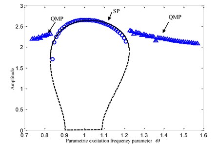
Fig. 9Comparison between analytical results and numerical solutions: (m=1, K1=1, α1=0.8, α2=0.01, B=0.4, K2=0.1, p=0.5, F=0.5)
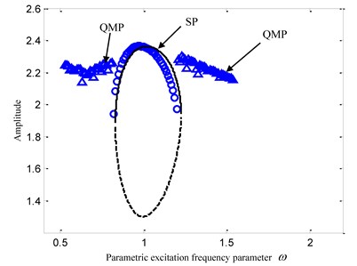
Fig. 10System response for ω= 0.875 and 0.87: Time history
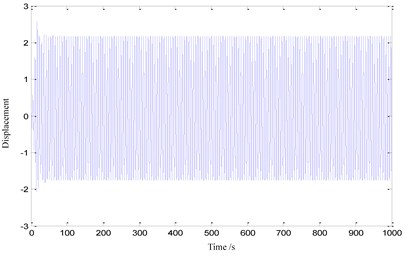
a) 0.875
b) 0.87
From the observation of Fig. 11, it could be found that the increase of would result into the rightward and downward movements of the amplitude-frequency curves. The main reason is that the ELSC will become larger with the increase of . Besides the above characteristics of the dynamical system responses, the topological structures of the amplitude-frequency curves vary significantly too. The increase of fractional-order coefficient would make the ovoid curve disappear, the open curve gradually turn up, and push the bifurcation point rightward. The proportion of steady-state solution in the amplitude-frequency curve is getting bigger and bigger with the increase of .
Fig. 11Influences of K2
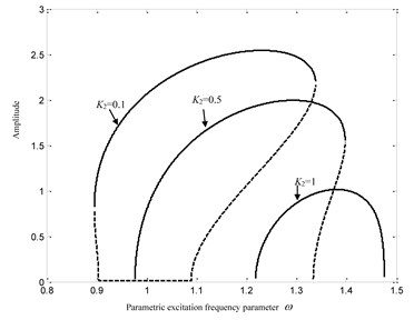
a)
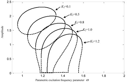
b)
When changes from 1 to 0, the amplitude-frequency curves of the fractional coefficient and are given in Fig. 12(a, b) respectively. The basic system parameters are selected as , , , , and . Through the analysis of Fig. 12, one can find that the decrease of will result into the rightward and upward movements of the amplitude-frequency curves. The open curve disappears, the ovoid curve gradually turns up, and the bifurcation point will move rightwards with the decrease of . Through the analysis of Eq. (17), one can find that the reason is that the ELSC will become larger, and the ELDC will become smaller when the fractional order . The ELSC will become smaller, and the ELDC will become larger when the fractional order . Accordingly, the decrease of will make the maximum response amplitude larger.
Fig. 12Influences of the fractional order p
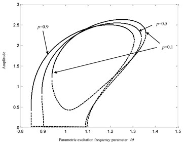
a) 0.1
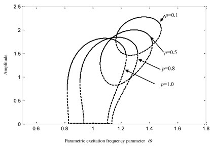
b)0.5
6. Conclusions
The dynamical characteristics of a Mathieu-van der Pol-Duffing fractional-order nonlinear system under 1/2 subharmonic resonance coupled with primary parametric resonance are investigated. The approximate analytical system solution is presented by the improved averaging approach. The numerical solutions are also studied by an iterative approach in three typical cases. The time history, phase portrait, FFT spectrum and Poincare maps are presented to identify the system response. There are Quasi-periodic, multi-periodic or single periodic behaviors. As the frequency is swept forward, the QMP response, SP response and QMP response will takes place in this system gradually, which is observed and investigated in three cases. Then the numerical results are compared with the analytical results. From three comparisons between the numerical and analytical results, one can find that the stable periodic solutions are in a good agreement with the numerical solutions, which verify the correctness and high accuracy of the approximate analytical solution. Finally, the influences of the fractional-order derivative parameters on the system dynamical response are analyzed. Through the analysis of the fractional-order derivative parameters, it can be found that the ELSC and ELDC both will become larger with the increase of fractional-order coefficient . The ELSC will become larger, and the ELDC will become smaller when the fractional order . The ELSC will become smaller, and the ELDC will become larger if the fractional order . A change of the fractional-order derivative parameters would lead to the motion of the amplitude-frequency curve and to a change of the topological structure of the amplitude-frequency curve. Those conclusions are very useful for the system design and control of the system dynamical response by choosing suitable fractional-order derivative parameters.
References
-
Petras I. Fractional-order Nonlinear Systems: Modeling, Analysis and Simulation. Higher Education Press, Beijing, 2011.
-
Caponetto R., Dongola G., Fortuna L., Petras I. Fractional Order Systems: Modeling and Control Applications. World Scientific, New Jersey, 2010.
-
Caputo M., Fabrizio M. A new definition of fractional derivative without singular kernel. Progress in Fractional Differentiation and Applications, Vol. 1, Issue 2, 2015, p. 73-85.
-
Yang X. J., Baleanu D., Srivastava H. M. Local Fractional Integral Transforms and Their Applications. Academic Press, London, 2015.
-
Agnieszka B., Malinowska, Delfim Torres F. M. Fractional calculus of variations for a combined Caputo derivative. Fractional Calculus and Applied Analysis, Vol. 14, Issue 4, 2011, p. 523-537.
-
Machado J. T., Kiryakova V., Mainardi F. Recent history of fractional calculus. Communications in Nonlinear Science and Numerical Simulation, Vol. 16, Issue 3, 2011, p. 1140-1153.
-
Yang J. H., Zhu H. The response property of one kind of fractional-order linear system excited by different periodical signals. Acta Physica Sinica, Vol. 62, Issue 2, 2013, p. 24501, (in Chinese).
-
Wang Z. H., Hu H. Y. Stability of a linear oscillator with damping force of fractional-order derivative. Science in China G: Physics, Mechanics and Astronomy, Vol. 39, Issue 10, 2009, p. 1495-1502, (in Chinese).
-
Shen Y. J., Wei P., Yang S. P. Primary resonance of fractional-order van der Pol oscillator. Nonlinear Dynamics, Vol. 77, Issue 4, 2014, p. 1629-1642.
-
Shen Y. J., Yang S. P., Sui C. Y. Analysis on limit cycle of fractional-order van der Pol oscillator. Chaos, Solitons and Fractals, Vol. 67, 2014, p. 94-102.
-
Li C. P., Deng W. H. Remarks on fractional derivatives. Applied Mathematics and Computation, Vol. 187, Issue 2, 2007, p. 777-784.
-
Deng W. H., Li C. P. The evolution of chaotic dynamics for fractional unified system. Physics Letters A, Vol. 372, Issue 4, 2008, p. 401-407.
-
Chen L. C., Hu F., Zhu W. Q. Stochastic dynamics and fractional optimal control of quasi integrable Hamiltonian systems with fractional derivative damping. Fractional Calculus and Applied Analysis, Vol. 16, Issue 1, 2013, p. 189-225.
-
Leung A. Y. T., Guo Z. J., Yang H. X. The residue harmonic balance for fractional order van der Pol like oscillators. Journal of Sound and Vibration, Vol. 331, Issue 5, 2012, p. 1115-1126.
-
You H., Shen Y. J., Yang S. P. Optimal design for fractional-order active isolation system. Advances in Mechanical Engineering, Vol. 7, Issue 12, 2015, p. 1-11.
-
Shen Y. J., Niu J. C., Yang S. P., Li S. J. Primary resonance of dry-friction oscillator with fractional-order PID Controller of velocity feedback. ASME Journal of Computational and Nonlinear Dynamics, Vol. 11, Issue 5, 2016, p. 51027.
-
Wang X. Y., Song J. M. Synchronization of the fractional order hyperchaos Lorenz systems with activation feedback control. Communications in Nonlinear Science and Numerical Simulation, Vol. 14, Issue 8, 2009, p. 3351-3357.
-
Yang X. J. Fractional derivatives of constant and variable orders applied to anomalous relaxation models in heat-transfer problems. Thermal Science, Vol. 21, Issue 3, 2017, p. 1161-1171.
-
Yang X. J., Machado J. A. T. A new fractional operator of variable order: application in the description of anomalous diffusion. Physica A: Statistical Mechanics and its Applications, Vol. 481, 2017, p. 276-283.
-
Li W., Zhang M. T., Zhao J. F. Stochastic bifurcations of generalized Duffing-van der Pol system with fractional derivative under colored noise. Chinese Physics B, Vol. 26, 2017, p. 90501.
-
Niu J. C., Shen Y. J., Yang S. P. Analysis of duffing oscillator with time-delayed fractional-order PID controller. International Journal of Non-Linear Mechanics, Vol. 92, 2017, p. 66-75.
-
Giresse T. A., Crépin K. T. Chaos generalized synchronization of coupled Mathieu-Van der Pol and coupled Duffing-Van der Pol systems using fractional order-derivative. Chaos, Solitons and Fractals, Vol. 98, 2017, p. 88-100.
-
Nayfeh A. H. Nonlinear Oscillations. Wiley, New York, 1973.
-
Chen Y. S. Nonlinear Vibrations. Higher Education Press, Beijing, 2002.
-
Li X. H., Hou J. Y., Shen Y. J. Slow-fast effect and generation mechanism of Brusselator based on coordinate transformation. Open Physics, Vol. 14, Issue 1, 2016, p. 261-268.
-
Li X. H., Hou J. Y. Bursting phenomenon in a piecewise mechanical system with parameter perturbation in stiffness. International Journal of Non-Linear Mechanics, Vol. 81, 2016, p. 65-176.
-
Belhaq M., Fahsi A. 2:1 and 1:1 frequency-locking in fast excited van der Pol-Mathieu-Duffing oscillator. Nonlinear Dynamics, Vol. 53, Issues 1-2, 2008, p. 139-152.
-
Wen S. F., Shen Y. J., Yang S. P., Wang J. Dynamical response of Mathieu-Duffing oscillator with fractional-order delayed feedback. Chaos, Solitons and Fractals, Vol. 94, 2017, p. 54-62.
-
Wen S. F., Shen Y. J., Li X. H., Yang S. P. Dynamical analysis of Mathieu equation with two kinds of van der Pol fractional-order terms. International Journal of Non-Linear Mechanics, Vol. 84, 2016, p. 130-138.
-
Xu Y., Li Y. G., Liu D., Jia W. T., Huang H. Responses of Duffing oscillator with fractional damping and random phase. Nonlinear Dynamics, Vol. 74, Issue 3, 2013, p. 745-753.
About this article

The authors are grateful to the support by the National Natural Science Foundation of China (No. 11602152), and the department project in Hebei Province (14212202D).
