Abstract
Bow-flare slamming of vessels is a reason of concern in the field of naval architecture. Severe slamming loads can result in not only local structure damages but also transient whipping loads. Global whipping oscillations increase both the extreme load and fatigue load effects occurring in ships. This paper provides an experimental investigation of bow-flare slamming loads and global hydroelastic vibrations of a vessel in severe irregular waves. Hydroelastic experiments by a segmented scaled model have been conducted in an ultra-long hydrodynamic basin. Responses of motion, acceleration, sectional load and slamming pressure of the model were measured corresponding to different wave conditions and sailing speeds. The characteristics of motions, accelerations and sectional loads under different conditions are analyzed by spectral method. The bow-flare slamming pressures are characterized and discussed from different aspects in detail. Moreover, the relationship between slamming pressures and the hull global responses is presented and discussed.
1. Introduction
Slamming is a strong nonlinear response of ship-wave interaction problem which can result in critical structural failure and onboard facilities damage. Slamming event occurs when the vessel motion causes an impact between the structural body and the water surface, and it is more likely to happen in case of high-speed vessels with flare-bow when sailing in harsh environment. On the other hand, for large and high-speed ships, slamming events can result in global whipping loads that may reach several times larger than the wave frequency loads. The whipping loads can also result in a significant reduction of the fatigue life of a vessel. Therefore, a better understanding of slamming and whipping responses of ships is of great importance for not only prototype design but also vessel appropriate operational guidelines [1].
During the past century, considerable efforts have been spent on investigating the slamming problems by researchers. The earliest study on slamming was carried out by the pioneering works of von Karman [2] and Wagner [3]. And then many analytical and numerical approaches were proposed based on their initial works [4, 5]. Up to now, two-dimensional wedge and revolving body water entry issues were well addressed by using numerical and experimental approaches [6-8]. However, owing to the complexity of the liquid-body interaction problem, the three-dimensional hydrodynamic impact issues are still far from being completely solved [9].
Due to the increasing dimensions of ships, hydroelastic effects must be considered while dealing with the slamming problems of large ships [10]. Numerical approaches were developed by researchers to simulate the slamming and whipping responses. Kim [11] investigated the slamming and whipping loads of ship in regular waves by fully coupled hydroelastic and experimental measurement. Piro and Maki [12] presented a hydroelastic analysis method for bodies entry and exit water analysis. Greco and Lugni [13] developed a three-dimensional seakeeping numerical solver to address the issue of water on deck and slamming.
Since the slamming and hydroelasticity issues of a large ship moving with forward speed in severe waves are complex to be addressed by numerical approach, experiments constitute an invaluable tool for the study of such issues. Tank model testing offers the opportunity to analyze slamming and whipping behaviors of ships with greater advantages over numerical approach and full-scale measurement. Luo [14] investigated the stern slamming and whipping effects of a containership model in both regular and irregular waves. Hong [15] studied the bow-flare slamming of a 10,000 TEU containership in regular waves. Lavroff [16] studied wave slamming loads on wave-piercer catamarans operating at high-speed by regular wave model tests. Hermundstad and Moan [17] studied the bow-flare slamming of a Ro-Ro vessel in regular oblique waves by numerical and experimental analyses. Drummen and Holtmann [18] carried out the benchmark study of slamming and whipping to study the accuracy of the extrapolation from the measured loads to the structural responses. A number of studies on the slamming impacts of ships in regular waves have been undertaken, however, only a few of publications studied the effects of slamming on motion and load responses of vessels in irregular waves [19, 20]. Dessi and Ciappi [21] studied the slamming clustering on fast ships through a novel analysis of the collected data from towing tank tests. Greco [22] carried out the seakeeping analysis of water on deck and slamming by numerical and physical investigation.
The primary objective of this work is to provide experimental reference data for bow-flare slamming loads and their effects on global responses of a large vessel sailing in severe irregular waves. In this paper, a hydroelastic segmented model of a vessel with pronounced flare bow has been developed and the tank experimental setup has been elaborately designed in order to obtain experimental data of the model in severe irregular waves. Motions, accelerations, loads and slamming pressures of the model for varying wave conditions and vessel speeds were measured and analyzed. The results indicate that the slamming induced whipping responses are pronounced in acceleration and load responses. Therefore, the relationship between slamming pressures and hull global responses is investigated.
2. Experimental setup
2.1. Test model
A 1:50 scaled geosim model was manufactured by using Fiberglass-Reinforced Plastics (FRP) to allow the measurement of slamming pressure and hull global responses experienced by a large vessel. Main particulars of prototype and the model are summarized in Table 1. More detailed parameters regarding the model can be found in the authors’ previous work [23].
Table 1Main particulars
Principal dimension | Prototype | Model |
Scale | 1/1 | 1/50 |
Length overall (m) | 313 | 6.26 |
Moulded breadth (m) | 39.5 | 0.79 |
Depth (m) | 25.5 | 0.51 |
Draft (m) | 10 | 0.20 |
Displacement (T) | 71875 | 0.575 |
As shown schematically in Fig. 1, the model was configured into seven separate segments, and cuts at stations #2, #4, #6, #8, #10 and #12 were provided. Gaps between each pair of segments were sealed using latex rubber which is elastic and waterproof. The segments were connected by a steel elastic backbone and the hull sectional bending load at each cut station can be measured by the strain gauges placed on the top and bottom surfaces of the backbone. The backbone was designed with varying cross-section so as to match the natural vibrational frequency and longitudinal stiffness distribution of vertical bending responses of the prototype. The backbone was rigidly fixed on the bottom bases of the segments at stations #1, #3, #5, #7, #9, #11 and #13 by using the dedicated fixing plates.
A monoblock segment from station #12 to #20 was adopted to house the propulsion system. The propulsion mechanism includes motors, shafts, cross-connect gearboxes, and propellers. During the tests, the thrust of the model was achieved by the propellers. The model is equipped with a total of four propellers to achieve the maximum testing speed. Twin rudders were also installed on the model to simulate the wake flow distribution near the propellers. Ballast iron blocks were installed inside the model to achieve the target center of gravity (COG) and radii of gyration so as to be similar with ship prototype.
Fig. 1Global view of model arrangement
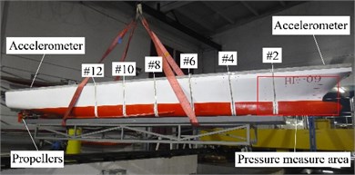
a) Photograph of the overall model
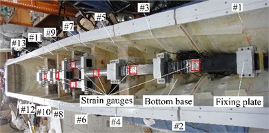
b) Backbone beam system
2.2. Test equipments
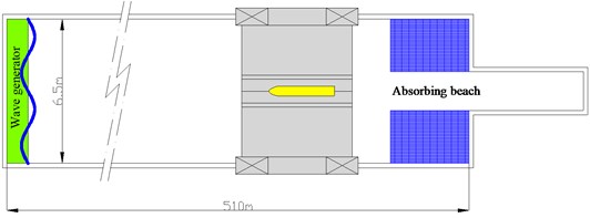
The experiments were conducted in the laboratory of high-speed hydrodynamic basin of Aviation Industry Institute No. 605, which is located in Jingmen, China. The dimensions of the tank are 510 m long, 6.5 m wide and 4 m water deep. The maximum speed allowable of the electric powered towing carriage is 16 m/s, and it has a speed accuracy of 0.001 m/s. During the tests, the speed of the carriage served as a reference, and the speed of the self-propelled model was controlled by an experienced staff via a dedicated motor control module. Both regular and irregular waves can be generated by a computerized single-flap type wave maker located at one end of the tank. A wave absorbing beach is positioned at the opposite side of the wave maker to prevent the reflecting of waves. The sketch of the ship hydrodynamic tank laboratory is shown in Fig. 2.
Fig. 2Sketch of the high-speed hydrodynamic tank laboratory
Motions of the model were measured by an in-house-developed four-degree-of-freedom (4-DOF) seaworthiness instrument, which also attached the model to the carriage. Pitch and heave motions were obtained by the mV/V signals of potentiometers mounted on heave stick and pitch pivot, respectively. The two sticks were installed respectively at stations #8.5 and #13.5 of the model, and they move freely in vertical and longitudinal directions. The heave motion at COG of the model can be derived by interpolation method using the data of the two known positions. Lateral movements of the model were restrained by the heave sticks. Therefore, the model was free to heave, pitch, roll and surge while being constrained in yaw and sway during the tests. View of the towing tank facility and the model setup are respectively shown in Figs. 3, 4.
The model was fully equipped with technique instruments to fulfill the required experimental measurement. A total of 10 pressure sensors were utilized and arranged on the bow area of the model. Nine were installed at the alternately wet and dry area to measure the bow-flare slamming pressure. They were arranged in the centerline plane (P1-P3 at bow front edge) as well as in three transverse planes (P4-P5 at station #0.6, P7-P8 at station #1.5 and P9-P10 at station #2.4). Another sensor was installed at the bow bottom (P6 at station #0.6) to measure the bottom fluctuating/slamming pressure. The locations of the pressure sensors are shown in Fig. 5. The pressure sensor comprises a pressure cell and a transducer amplifier, and is shown in Fig. 6. Technical data regarding the pressure sensors are listed in Table 2.
Fig. 3Towing carriage facility
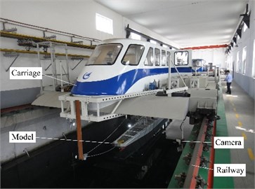
Fig. 4Photograph of test setup
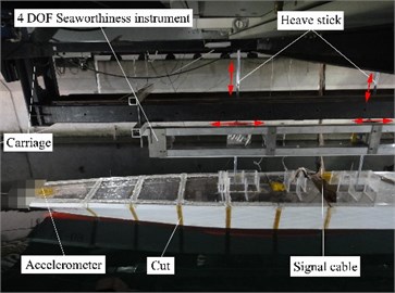
Fig. 5Arrangement of pressure sensors
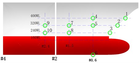
Fig. 6Pressure sensor
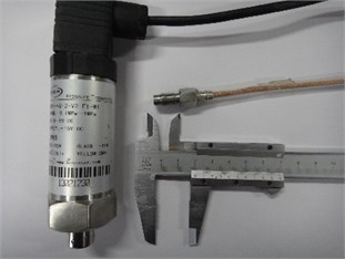
Table 2Technique data of the pressure sensor
Index | Parameter |
Measuring medium | Gas or liquid |
Scale range (m H2O) | –10-10 |
Input voltage (V DC) | ±15 |
Output signal (V DC) | –0.5-5 |
Measurement accuracy (FS) | ±0.25 % |
Operating temperature range (°C) | –20-80 |
Frequency (Hz) | 10-20000 |
Sectional vertical bending moment (VBM) at each of the six cut sections was measured by strain gauges placed onto the backbone surface. A full-bridge circuit was adopted to achieve high measurement accuracy and high stability. The measured strain signal was transformed to VBM by considering the Young modulus and geometric cross-section parameters of the backbone beam. Calibration tests were also conducted on the beam prior to the tank tests by applying known static loads and recording the corresponding strain values to validate the calculated conversion coefficients.
Vertical accelerations at two points, the station #1 at the bow and the station #19 at the stern, were measured by axis accelerometers mounted on centerline of the primary deck. The accelerometer has an output coefficient of 2000 mV/g. Technical data regarding the accelerometers utilized are listed in Table 3.
During the tests, sampling frequencies of motions, loads and accelerations were set at 50 Hz, while the sampling frequency of pressures was set at 1000 Hz in order to capture the peak value of slamming. All the acquired signals were transmitted to a data collector in the operational room onboard the carriage via a local signal cable.
Table 3Technique data of the accelerometer
Index | Parameter |
Range (g) | ±2 |
Maximum range (g) | ±20 |
0g output (mVDC) | –1 |
Output impedance (Ω) | ≤ 300 |
Transverse sensitivity (%) | ≤ 3.0 |
Operating temperature range (°C) | –55-125 |
Mounted resonant frequency (kHz) | 1.3 |
2.3. Test scheme
Tests were conducted corresponding to two control strategies, i.e. wave condition and vessel sailing speed. Control parameters of the scaled model were determined according to the similitude law in the knowledge of ship hydrodynamic experiment. In order to study the slamming and global responses of the vessel under different sea states, tests were conducted corresponding to real ship significant wave height from 6 m to 20 m. For each of the full-scale significant wave height, the corresponding wave mean period was determined according to the most probable one from the scatter diagram of the North Atlantic sea states. ISSC double-parameter spectra were adopted to simulate the time series of irregular waves. The testing speed for the majority of cases is 18 knots corresponding to real ship, which is the designed cruising speed. In addition, three speeds, i.e. 18 knots, 24 knots and 30 knots, were investigated for 12 m significant wave height. The test conditions studied in this paper are listed in Table 4.
It is noted that all the cases were tested for head wave conditions. For each of the test condition, one run was conducted in the ultra-long distance tank. With the exception of the acceleration and deceleration regions, the steady-run testing region is over 300 m for each of the test scheme. At least 150 waves were encountered by the model during the steady-run region to ensure the statistical representation of the measured data.
Table 4Test conditions
Testing ID | Full-scale prototype | Scaled model | ||||
(m) | (s) | (knot) | (mm) | (s) | (m/s) | |
1 | 6 | 9.5 | 18 | 120 | 1.34 | 1.309 |
2 | 8 | 10.5 | 18 | 160 | 1.48 | 1.309 |
3 | 10 | 10.5 | 18 | 200 | 1.48 | 1.309 |
4/5/6 | 12 | 11.5 | 18/24/30 | 240 | 1.63 | 1.309/1.746/2.182 |
7 | 14 | 11.5 | 18 | 280 | 1.63 | 1.309 |
8 | 16 | 12.5 | 18 | 320 | 1.77 | 1.309 |
9 | 18 | 12.5 | 18 | 360 | 1.77 | 1.309 |
10 | 20 | 13.5 | 18 | 400 | 1.91 | 1.309 |
3. Examples of measured time series
In order to investigate the relationship between motion, acceleration, sectional load and slamming pressure, examples of the measured time series of one typical testing case (significant wave height 240 mm and sailing speed 1.309 m/s) are illustrated in this section, and all the raw experimental data are given in model scale. The comprehensive analyses regarding the slamming characteristics as well as the hull global responses will be described in the next two sections.
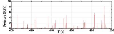
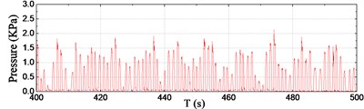
For the sake of simplicity, six typical channels of pressure data within 100 s during the steady-run region are selected and shown in Fig. 7. As seen from the results, a number of slamming events have taken place during the 100 s records. According to the pressure results at the front edge, the wave impact occurrence frequency increases distinctly from P1 to P3, however, the maximum peak value of slamming pressure during the 100 s decreases from P1 to P3, i.e. from 8.27 kPa at P1 to 5.00 kPa at P3. The slamming occurrence frequency at P3 and P8 is almost the same, whereas the peak value at P3 is obviously greater than that of P8 for each corresponding impact. It is noted that P6 was immersed in the water all along this duration, so the recorded time series of fluctuating pressure seems to be smooth.
Fig. 7Pressure time series
a) Sensor P1
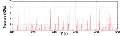
b) Sensor P2
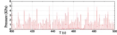
c) Sensor P3
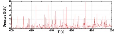
d) Sensor P5
e) Sensor P6
f) Sensor P8
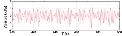
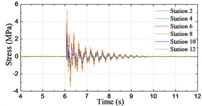
Fig. 8Time series of sectional loads
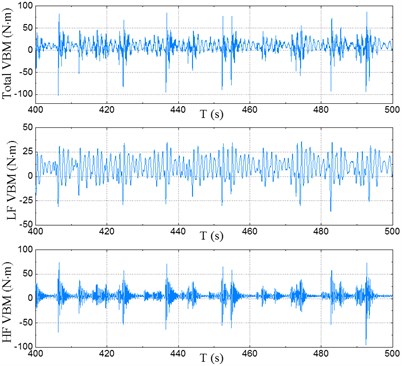
a) At station #2
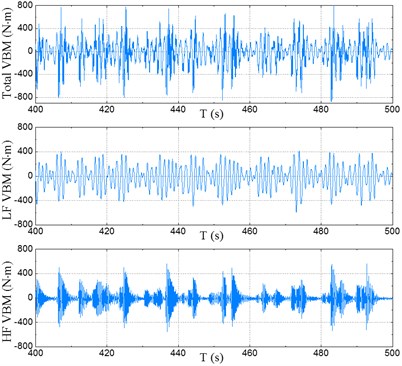
b) At station #10
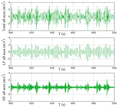
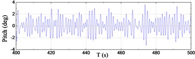
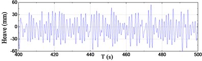
Time series of sectional VBM at typical stations #2 and #10 are plotted in Fig. 8. The fast Fourier transform (FFT) filter was used to separate the low-frequency (LF) components caused by waves and the high-frequency (HF) whipping components caused by slamming. In these figures – for the sake of clarification – total load (raw data), LF load and HF load are illustrated in the order from top to bottom, respectively. Time series of accelerations at bow and aft areas are presented in Fig. 9. LF and HF components of accelerations were also separated by using of the FFT filter and the results are shown in these figures. Time series of motion responses, i.e. pitch and heave at COG of the model, are depicted in Fig. 10.
As seen from the illustrated time series in Fig. 7-10, whipping is pronounced in the responses of sectional loads and vertical accelerations rather than the motion. The HF whipping components of load and acceleration caused by bow-flare slamming increase the total responses significantly, and they are of the same order of the LF components. Moreover, the HF components are more pronounced at bow area than amidships and aft areas. On the other hand, it is clear that there is no HF component in the motion responses, i.e. the motion curves are stationary and smooth even after the occurrence of slamming.
Fig. 9Time series of accelerations
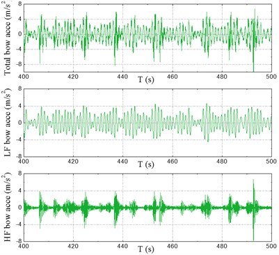
a) At bow
b) At stern
Fig. 10Time series of motions at COG
a) Pitch
b) Heave at COG
4. Analyses of experimental results
4.1. Identification of the resonance frequencies
Impact hammer tests were conducted when the model was in still water without forward speed to determine at which frequencies the vertical resonances occur. As a matter of fact, it has already been verified that forward speed has very little effects on the frequency of the first-order bending mode [16]. During the mode test, a soft hammer was used to hit the bow center area of the model and recorded the decay oscillation time series using strain gauges placed on the backbone beam. In order to visualize the frequency-domain information in detail, FFT method was used to process the measured time series data. Since some measuring locations may be at or near the vibrational nodes, it is better to refer the frequency-domain outcomes of stress at all the recorded positions along the model so as to determine the resonance frequencies comprehensively [24].
The measured decay curves at different stations and the corresponding frequency-domain results by FFT are shown in Fig. 11, and the results are given in model scale. As seen from the results, there are obvious peaks at the two node vertical vibration frequency 24.16 rad/s (3.87 Hz) and the three node vertical vibration frequency 58.92 rad/s (9.38 Hz).
Fig. 11Hammer test results of vertical vibrations in calm water
a) Decay curves of sectional stress
b) Frequency-domain results by FFT
4.2. Analysis of motion, acceleration and load responses
In order to obtain the frequency-domain information as well as the statistical significant values of motions, accelerations and loads, an in-house code based on auto-correlation function algorithm was adopted. The basic equations regarding the auto-correlation function method are summarized in the following statements [25].
As is well known, the variance spectrum can be obtained by carrying out the Fourier transformation of the auto-correlation function, which is expressed as follows:
where denotes the frequency spectrum, denotes the frequency, denotes the auto-correlation function, and denotes the time interval between two given points.
According to the theory of probability, the auto-correlation function of variables is expressed as:
where denotes the acquiring of mathematical expectation, and denotes the value in the time series at the time .
The auto-correlation function can be written as follows by assuming that the signal processed is ergodic and stationary random process:
where denotes the time duration of the measured time series.
The time interval is after dividing the time duration into partitions. The mean representative time of the classified intervals in the order from the beginning to the end over the whole process range are , ,…, , respectively. Then, using , ,…, to replace and substituting them into Eq. (3), the following equation can be obtained:
where denotes the largest interval number.
The auto-correlation values of for 0, 1,…, can be obtained by Eq. (4), and then substituting these values into Eq. (1). Besides, trapezoidal quadrature method is used to obtain the spectrum:
Since the initial spectrum by Eq. (5) is not smooth, the Hamming smoothing is adopted to process the initial spectrum. The equations for smoothing can be derived as:
where denotes the final spectrum after smoothing.
In addition, the significant amplitude value can be obtained based on the acquired spectral result, written as:
where denotes the significant amplitude value, and denotes the 0th moment of the spectrum, i.e. the area below the spectral curve.
Fig. 12Motion and acceleration spectra for different conditions
a) Pitch
b) Heave at COG
c) Bow acceleration
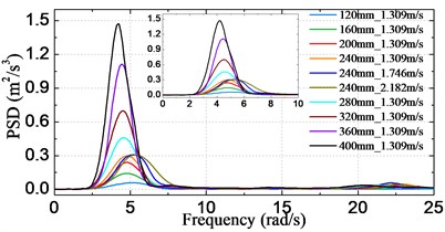
d) Stern acceleration
4.2.1. Motion and acceleration responses
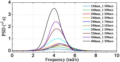
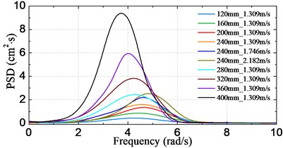
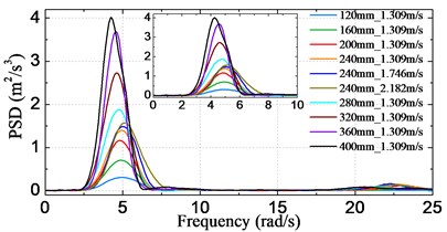
Fig. 12 shows the obtained frequency spectra of motion and acceleration by the above-mentioned spectral method. The results are given corresponding to model scale. In these figures, spectral curves of all the test schemes for each signal are plotted together for the sake of comparison, and the axis denotes the encounter frequency (). The results indicate that the peak frequency of curves decreases with increasing significant wave height, however, it rises with increasing sailing speed. This can be explained by the fact that the dominant encounter frequency varies with different incident wave states or different sailing speeds. Another feature of the curves is that the peak value increases for both increasing significant wave height and sailing speed. Moreover, it is noted that – unlike the pitch and heave spectra – there exist HF components at around the two node vibrational frequency of the acceleration spectra, which is in accordance with the phenomenon observed from the results in Fig. 9.
The statistical significant amplitude values of motions and accelerations obtained by using of Eq. (7) are plotted in Fig. 13-14, respectively for varying significant wave height cases and sailing speed cases. It can be clearly seen from Fig. 13 that the statistical significant amplitude value is almost proportion to the significant wave height for all of the four signals. On the other hand, as seen from Fig. 14, heave and acceleration values increase linearly with increasing sailing speed, however, the pitch shows an opposite trend. This is attributable to the fact that the encounter frequency departs from the resonant frequency of pitch when speed is increased from 1.309 m/s (18 knots at full-scale) to 2.182 m/s (30 knots at full-scale), therefore, the largest pitch appears at the speed of 1.309 m/s.
Fig. 13Significant amplitude values of motion and acceleration responses against the wave height
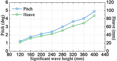
a) Pitch and heave at COG
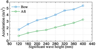
b) Accelerations at bow and stern
Fig. 14Significant amplitude values of motion and acceleration response against the speed
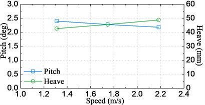
a) Pitch and heave at COG
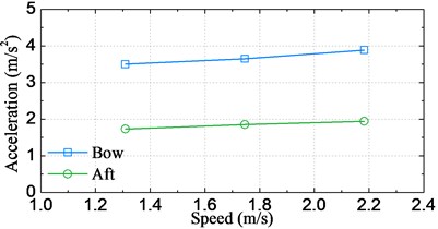
b) Accelerations at bow and stern
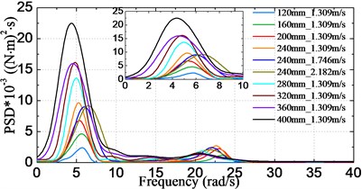
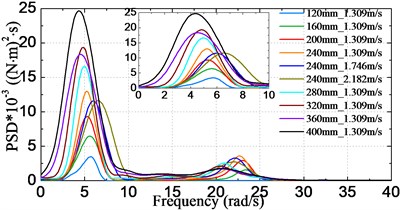
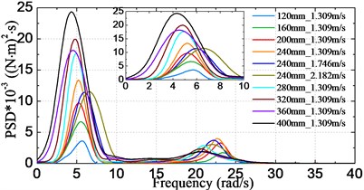
4.2.2. Load responses
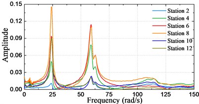
Fig. 15 shows the obtained frequency spectra of VBM ranged at stations #2, #4,…, #12. The results are given corresponding to model scale. Some common characteristics regarding the HF components can be found between the load spectra and the acceleration spectra: HF components are mainly congregated at around the two node vibrational frequency. The HF energy in the load spectra is more pronounced than that in the acceleration spectra. In addition, there are more HF components at or near the bow area due to bow-flare slamming, and the curves around the bow area are more irregular than those at stations near the amidships area.
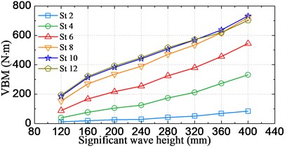
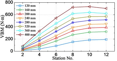
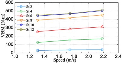
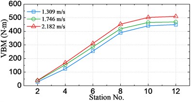
Figs. 16, 17 respectively show the changes of statistical significant amplitude values of VBM obtained by Eq. (7) varying with the significant wave height and the sailing speed. The results in Fig. 16(a) and 17(a) indicate that the significant amplitude values increase with increasing significant wave height and sailing speed. There is a noticeable trend that the values increase faster under higher seas than moderate seas, which can be attributed to the nonlinear wave loads acting on the vessel. On the other hand, as seen from Fig. 16(b), the largest significant amplitude value took place at station #12 for cases of significant wave height less than 320 mm (16 m at full-scale), while it moves towards the bow direction for cases of higher significant wave height, i.e. it occurred at station #10 (amidships section) for cases under significant wave height 360 mm (18 m at full-scale) and 400 mm (20 m at full-scale).
Fig. 15Load spectra at different stations
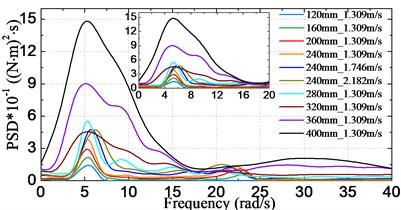
a) Station #2
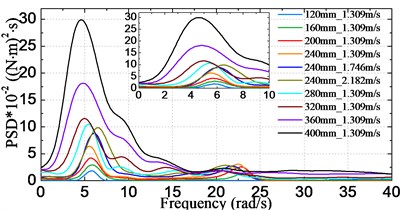
b) Station #4
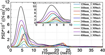
c) Station #6
d) Station #8
e) Station #10
f) Station #12
Fig. 16Significant amplitude values of VBM for different wave states
a) Against the significant wave height
b) Against the station
4.3. Analysis of slamming pressure characteristics
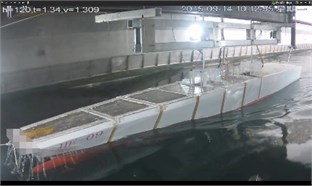
During the tests, the experimental process was also recorded by a dedicated video camera – at left front side of the model – fixed on the carriage. Playback of the video recordings reveals the following phenomenon: when the ship sailed with large amplitude coupled pitch and heave motions, violent bow flare impact would occur due to the relative motion of the model with respect to the incoming waves. During a slamming cycle, once the bow was at the trough of a wave it emerged from the water, and then hit the incoming wave crest at a relative high velocity.
Fig. 17Significant amplitude values of VBM at different speeds
a) Against the speed
b) Against the station
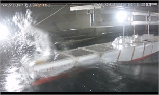
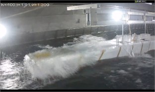
Slamming phenomena under different conditions captured from the video recordings are shown in Fig. 18. To summarize, only slight slamming event happened when the significant wave height was less than 160 mm (8 m at full-scale). Slamming became more pronounced with increasing significant wave height. When the significant wave height was greater than 320 mm (16 m at full-scale), the bow had already pierced the water and thereby resulted in severe slamming and shipping water on deck. In addition, from carefully observation of the video recordings for different sailing speeds, the slamming phenomenon became more severe with increasing speed from 1.309 m/s (18 knots at full-scale) to 2.182 m/s (30 knots at full-scale) for significant wave height of 240 mm (12 m at full-scale), which can be observed from Fig. 18 (d)-(f).
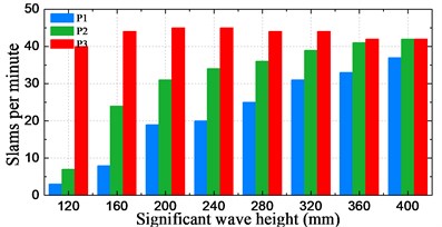
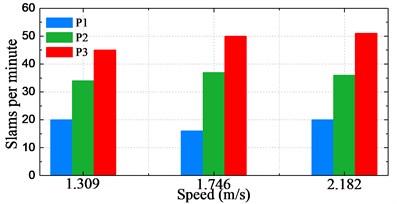
The frequency of slamming event occurrence at P1-P3 was counted from the steady-run region of each time series recorded. Fig. 19 shows an overview of the statistical description of slamming occurrence frequency varying with significant wave height and sailing speed. Fig. 19(a) indicates that the water impact frequency at P3 fluctuated between 40 and 45 over all the cases with the sailing speed of 1.309 m/s (18 knots at full-scale). This can be attributed to the fact that almost every pitch motion would result in water entry of P3 since it is very near to the waterline. The impact frequency shows a linear growth against the increasing significant wave height at P1. The impact frequency at P2 experiences a sharp rise from the significant wave height of 120 mm (6 m at full-scale) to 160 mm (8 m at full-scale), and then it rises gradually, finally with the significant wave height 400 mm (20 m at full-scale), it achieved the same frequency as that of P3. Fig. 19(b) shows that the impact frequencies at P2 and P3 witness a slight and steady growth from the speed of 1.309 m/s (18 knots at full-scale) to 2.182 m/s (30 knots at full-scale). However, the frequency at P1 shows a small fluctuation with the increasing of speed.
4.3.1. Distribution of largest pressure peaks
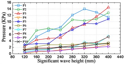
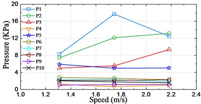
In order to study the distribution of the pressure peak values, the maximum peak values at sensors P1-P5 and P7-P10 and the largest peak-to-peak value at sensor P6 during the steady-run region of the measured time series were extracted. Fig. 20 shows the largest pressure peaks against the significant wave height and the sailing speed for all the sensors.
As seen from Fig. 20(a), for sensors P3-P10 the largest pressure peak value rises with increasing significant wave height. However, the curves at P1 and P2 revealed a fluctuation of trend with increasing significant wave height. For instance, the slamming pressure peak value at P1 for significant wave heights of 360 mm (18 m at full-scale) and 400 mm (20 m at full-scale) is even smaller than that of 320 mm (16 m at full-scale). This can be attributed to the randomicity and nonlinear effects of severe slamming. In spite of the sharp fluctuations of curves at P1 and P2, the trend is obviously upwards. Fig. 20(b) shows the largest pressure peak value against the increasing sailing speed from 1.309 m/s (18 knots at full-scale) to 2.182 m/s (30 knots at full-scale) for significant wave height 240 mm (12m at full-scale). It is of interest to note that increasing sailing speed has little influence on the peak pressures at P4-P10. Moreover, the peak pressures at P5, P6 and P10 even decrease slightly with increasing sailing speed. The peak pressures at P2 and P3 show a pronounced rise with increasing sailing speed. However, the largest peak pressure at P1 reaches the maximum value at the speed of 1.746 m/s (24 knots at full-scale).
Fig. 18Snapshots captured from the video recordings
a) 120 mm_1.309 m/s
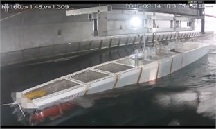
b) 160 mm_1.309 m/s
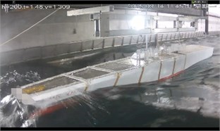
c) 200 mm_1.309 m/s
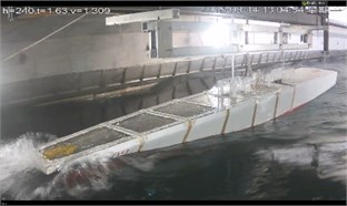
d) 240 mm_1.309 m/s
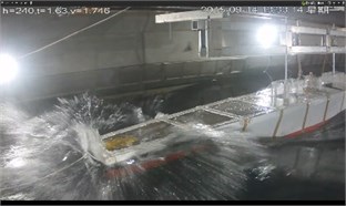
e) 240 mm_1.746 m/s
f) 240 mm_2.182 m/s
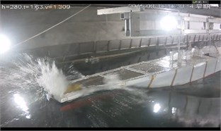
g) 280 mm_1.309 m/s
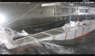
h) 320 mm_1.309 m/s
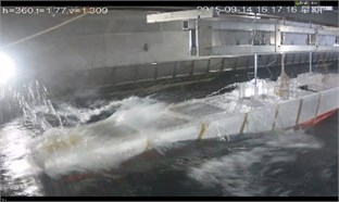
i) 360 mm_1.309 m/s
j) 400 mm_1.309 m/s
Fig. 19Statistical results of slamming frequency
a) Against the significant wave height
b) Against the sailing speed
Fig. 20Distributions of largest pressure peak values
a) Against the wave height
b) Against the speed
4.3.2. Spatial distribution of notable enormous pressure peaks
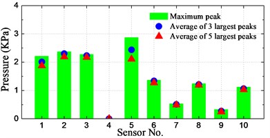
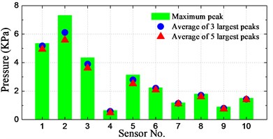
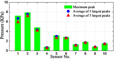
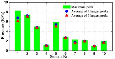
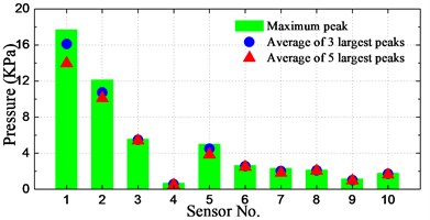
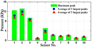
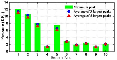
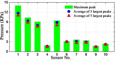
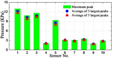
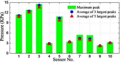
The spatial distribution of slamming pressure peaks is a reason of concern in this study. In order to investigate the spatial distributions of the notable enormous impact pressures, the maximum peak as well as the averages of first-three and first-five largest peaks at the 10 sensors for different conditions are calculated and illustrated in Fig. 21.
As seen from the histograms, the largest pressure for cases of significant wave height 160-400 mm (8 m-20 m at full-scale) occurred at positions P1-P3, which are located at the bow front edge. For the case of significant wave height of 6 m, the largest pressure took place at position P5, which has the lowest dead rise angle among these sensors. Overall, the relative small peak value took place at positions P4 and P9, which are located farthest from the waterline and farthest from the bow front edge, respectively.
It can be seen that the averages of 3 and 5 largest peaks are not so different with the maximum pressure peak at P4 and P6-P10, while the difference is pronounced at P1-P3 and P5 for most of the conditions. It indicates that the magnitudes of measured slamming pressure peaks are scattered noticeably large at P1-P3 and P5. It is also interesting to note that the pressures at P1-P3 and P5 are obviously larger than those of other sensors for all the conditions.
In summary, it can be generalized that the relative high pressures take place at the bow front edge or at the section with smallest dead rise angle. The peak value distribution at these positions has a large range of magnitudes.
4.3.3. Probability density distribution of peak values
To investigate the characteristics of probability density distribution of pressure peaks, the peak values of the four typical pressure sensors of P1-P3 and P5, which have relatively strongly nonlinear and large magnitude features, were extracted from the steady-run region of time series. For the sake of simplicity, only the most severe condition – significant wave height of 400 mm (20 m at full-scale) and sailing speed of 1.309 m/s (18 knots at full-scale) – is selected for this study.
The peak values at P1-P3 and P5 at different slams are shown in Fig. 22. A total of 143 slamming events have been taken place during the run. It is clear that the association between the peak values of the four sensors is weak. For example, the ratios of the four pressure values vary for different slamming events, i.e. for some of the slams the largest pressure happened at P1, while for others it happened at P2 or P3.
Fig. 21Spatial distribution of notable enormous pressure peaks
a) 120 mm_1.309 m/s
b) 160 mm_1.309 m/s
c) 200 mm_1.309 m/s
d) 240 mm_1.309 m/s
e) 240 mm_1.746 m/s
f) 240 mm_2.182 m/s
g) 280 mm_1.309 m/s
h) 320 mm_1.309 m/s
i) 360 mm_1.309 m/s
j) 400 mm_1.309 m/s
Graphical representations of the statistical peak values with histograms are shown in Fig. 23. Each figure presents the frequency of occurrence of peak values in different intervals counted from the results in Fig. 22. In addition, the corresponding fitted results by the Weibull function are also plotted in the figures. The statistical histograms show acceptable agreement with the fitted Weibull distribution. However, since the available samples are limited, the results show imperfect distribution in the figures.
Fig. 22Pressure peak values at different slams
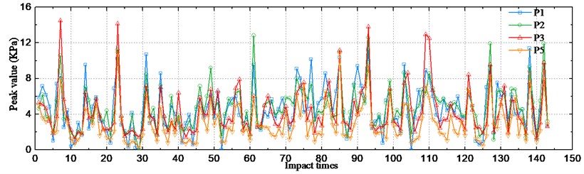
Fig. 23Histograms of pressure peak value distribution
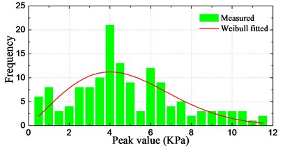
a) Sensor P1
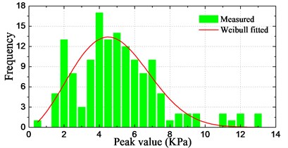
b) Sensor P2
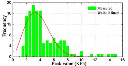
c) Sensor P3
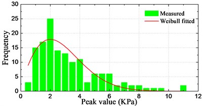
d) Sensor P5
5. Relationship between impact pressures and global responses
Prior to investigating the relationship between impact pressure and global vibrations, it is critical to understand under what circumstance the water impact would take place. Since slamming is induced by large amplitude motions, Fig. 24 illustrates the values of pitch and heave motions versus the impact pressure within 20 s from the example time series data in Section 3. In the figure, the pressure at P2 is selected as the typical pressure for slamming identification. It is noted that the positive/negative value of pitch represents trim by the stern/bow, and the positive/negative value of heave represents COG situated above/below the mean position.
As seen from the time series in Fig. 24, the pitch and heave are coupled all along and they reach the crest or trough positions nearly at the same moment. To summarize, prior to slamming impact, the pitch and heave motions reach a maximum value in the time series, which means that the bow is relative far from the mean water surface and thus with a maximum potential energy at that time. Then the slamming occurs when the ship bow moves down towards the wave. Owing to the fact of impact with water, the vertical downward velocity of bow decreases rapidly. Once the pitch and heave reach the trough position, the motion changes direction to a bow up motion due to the restoring force and moment.
The peak values of slamming pressure were extracted from the time series. In addition, the corresponding positive and negative peaks of the pitch and heave motions that resulted in each of the slamming event were also extracted. The identified results given in Fig. 24 are marked with symbols. Then the peak-to-peak values of motions were derived as the characteristic values corresponding to each slamming event. The statistical scatter grams of peak pressures at P1-P3 versus the peak-to-peak values of motions are shown in Fig. 25. It can be found that the relationship between slamming pressure peaks and the motions is as follows: for P1 and P2 the distribution of scatter points is weak associated, while for P3 they have a correlation. The trend shows that an average large amplitude motion can result in relative higher pressure peak at P3, but also shows that the large/small amplitude motion do not always result in high/low pressure peak at P1 and P2. It is likely that besides the motion magnitude there exist other factors that affect the slamming pressure magnitude, for instance, the impact period, the incoming wave, the vertical velocity and the motion information 2-3 periods before the slamming event.
Fig. 24Time series of slamming pressure and motions at COG
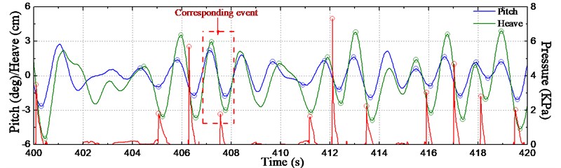
Fig. 25Relationship between the slamming pressure and motions
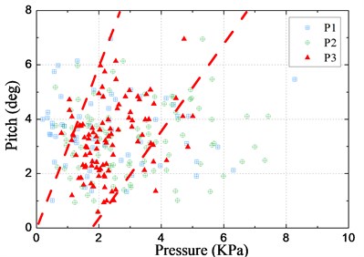
a) Relation with pitch
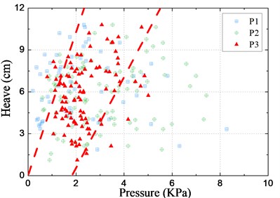
b) Relation with heave at COG
Fig. 26 shows the time series of whipping loads at station #10 versus the pressure value at P2 using the example data in Section 3, with a positive/negative value of sectional load representing hogging/sagging bending moment. As seen from the figure, the rapid increasing whipping load occurs after the occurrence of slamming impact and then decays rapidly due to the hydrodynamic and structural dampings. The vibrations superimpose when another slamming occurs. The positive and negative peaks of the whipping loads induced by each of the slamming event were extracted and marked with symbols in the figure.
The statistical scatter grams of pressure peaks at P1-P3 and the corresponding peak-to-peak values of whipping loads of typical stations #2 and #10 are shown in Fig. 27. It is observed that the slamming peak pressures and the whipping loads have a clear correlation as follows: the magnitude of loads shows raising trend with increasing impact pressure. At impact pressure lower than 3 kPa, however, a few large loads are also observed. This can be interpreted as the VBM induced by springing.
Fig. 26Time series of slamming pressure and whipping load at station #10
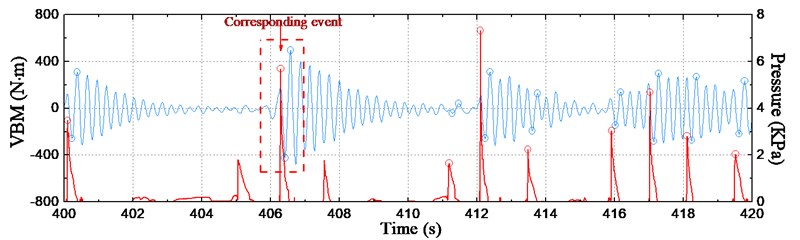
Fig. 27Relationship between the slamming pressure and whipping loads
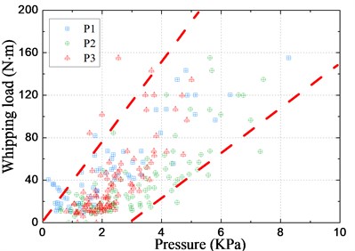
a) Relation with load at station #2
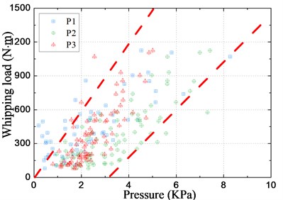
b) Relation with load at station #10
6. Conclusions
Tests of a segmented ship model in severe irregular waves have been conducted for the investigation of bow-flare slamming and hydroelastic vibration responses. The slamming and whipping characteristics of the full-scale ship were replicated in the model through the dedicated tank experimental setup. On the basis of the obtained test results the following conclusions can be made:
1) From the measured time series of motion, acceleration and load and their spectra results, it is obvious that slamming has more effects on accelerations and loads than motions. The HF whipping components of load and acceleration caused by bow-flare slamming increase the total responses significantly. The vibrational frequency of the HF whipping components of all the test conditions is found to be close to the two node natural vibrational frequency identified by hammer test.
2) The significant amplitude values of pitch and heave motion, acceleration and load rise with increasing significant wave height. Also the significant amplitude values of heave motion, acceleration and load rise with increasing sailing speed. However, the pitch motion decreases with increasing sailing speed.
3) Increasing the significant wave height has pronounced effects on the largest pressure peak values at all the sensors. However, the influence of increasing speed is mainly distinct for the pressures at the front edge area. In addition, the relative high pressures occur at the front edge or at the cross-section with smallest dead rise angle. The temporal distribution of pressure peak values at these positions has a large range of magnitudes.
4) Average large amplitude motions can result in relative higher pressure peak at P3, however, the large/small amplitude motion do not always result in high/low pressure peak at P1 and P2. As for the relationship between slamming peak pressures and the whipping loads, they have a clear correlation: the magnitude of loads shows a rising trend with increasing impact pressure at the front edge. To conclude, more analysis regarding the relationship between the impact pressure and hull global responses is needed. Future study will also be devoted to identify the springing and whipping vibrations.
References
-
Thomas G., Winkler S., Davis M., Holloway D., Matsubara S., Lavroff J., French B. Slam events of high-speed catamarans in irregular waves. Journal of Marine Science and Technology, Vol. 16, 2011, p. 8-21.
-
Karman V. The Impact on Seaplane Floats during Landing. NACA Technical Note No. 321, 1929.
-
Wagner H. Uber stoss-und gleitvorgange an der oberflache von flussigkeiten. ZAMM, Vol. 12, Issue 4, 1932, p. 193-235, (in German).
-
Xu G., Duan W. Review of prediction techniques on hydrodynamic impact of ships. Journal of Marine Science and Application, Vol. 8, Issue 3, 2009, p. 204-210.
-
Luo H., Xu H., Yu J., Wan Z. Review of the state of the art of dynamic responses induced by slamming loads on ship structures. Journal of Ship Mechanics, Vol. 14, Issue 4, 2010, p. 439-450.
-
Mei X., Liu Y., Yue D. On the water impact of general two-dimensional sections. Applied Ocean Research, Vol. 21, 1999, p. 1-15.
-
Zhao R., Faltinsen O. Water entry of two-dimensional bodies. Journal of Fluid Mechanics, Vol. 246, 1993, p. 593-612.
-
Wu G., Sun H., He Y. Numerical simulation and experimental study of water entry of a wedge in free fall motion. Journal of Fluids and Structures, Vol. 19, 2004, p. 277-289.
-
Kapsenberg G. Slamming of ships: where are we now? Philosophical Transactions of the Royal Society A, Vol. 369, 2011, p. 2892-2919.
-
Cui W., Yang J., Wu Y., Liu Y. Theory of Hydroelasticity and its Application to Very Large Floating Structures. Shanghai Jiao Tong University, Hanghai, China, 2007.
-
Kim J., Kim Y., Yuck R., Lee D. Comparison of slamming and whipping loads by fully coupled hydroelastic analysis and experimental measurement. Journal of Fluids and Structures, Vol. 52, 2015, p. 145-165.
-
Piro D., Maki K. Hydroelastic analysis of bodies that enter and exit water. Journal of Fluids and Structures, Vol. 37, 2013, p. 134-150.
-
Greco M., Lugni C. 3-D seakeeping analysis with water on deck and slamming. Part 1: Numerical solver. Journal of Fluids and Structures, Vol. 33, 2012, p. 127-147.
-
Luo H., Qiu Q., Wan Z., Yang D. Experimental investigation of the stern slamming and whipping in regular and irregular waves. Journal of Ship Mechanics, Vol. 10, Issue 3, 2006, p. 150-162.
-
Hong S., Kim K., Kim B., Kim Y. Experiment study on the bow-flare slamming of a 10,000 TEU containership. Proceeding of the 24th International Ocean and Polar Engineering Conference, 2014, p. 816-823.
-
Lavroff J., Davis M., Holloway D., Thomas G. Wave slamming loads on wave-piercer catamarans operating at high-speed determined by hydro-elastic segmented model experiments. Marine Structures, Vol. 33, 2013, p. 120-142.
-
Hermundstad O., Moan T. Numerical and experimental analysis of bow flare slamming on a Ro-Ro vessel in regular oblique waves. Journal of Marine Science and Technology, Vol. 10, 2005, p. 105-122.
-
Drummen I., Holtmann M. Benchmark study of slamming and whipping. Ocean Engineering, Vol. 86, 2014, p. 3-10.
-
Hong S., Kim K., Kim B., Kim Y. Characteristics of bow-flare slamming loads on an ultra-large containership in irregular waves. Proceeding of the 25th International Ocean and Polar Engineering Conference, 2015, p. 75-81.
-
Chiu F., Tiao W., Guo J. Experimental study on the nonlinear pressure acting on a high-speed vessel in irregular waves. Journal of Marine Science and Technology, Vol. 14, 2009, p. 228-239.
-
Dessi D., Ciappi E. Slamming clustering on fast ships: from impact dynamics to global response analysis. Ocean Engineering, Vol. 62, 2013, p. 110-122.
-
Greco M., Bouscasse B., Lugni C. 3-D seakeeping analysis with water on deck and slamming. Part 2: Experiments and physical investigation. Journal of Fluids and Structures, Vol. 33, 2012, p. 148-179.
-
Jiao J., Ren H., Adenya C. Experimental and numerical analysis of hull girder vibrations and bow impact of a large ship sailing in waves. Shock and Vibration, Vol. 2015, 2015, p. 1-10.
-
Maron A., Kapsenberg G. Design of a ship model for hydro-elastic experiments in waves. International Journal of Naval Architecture and Ocean Engineering, Vol. 6, 2014, p. 1130-1147.
-
Li J. Seakeeping Performance of Ships. Harbin Engineering University, Harbin, China, 2003.
Cited by
About this article

The authors would like to thank Technical Engineer Zhao Xiaodong and all the experimental participants in the Institute of Naval Architecture and Ocean Engineering Mechanics (INOM) of Harbin Engineering University (HEU) for their kind help during the preparation and performance of the tests. This work was partly supported by the National Natural Science Foundation of China (No. 51079034).
