Minh Hung Vu | Ngoc Thai Huynh | Khoi Nguyen Nguyen | Anh Son Tran | Quoc Manh Nguyen*
© 2022 IIETA. This article is published by IIETA and is licensed under the CC BY 4.0 license (http://creativecommons.org/licenses/by/4.0/).
OPEN ACCESS
The steering system in the car assumes the task of navigating when the car is in motion. It not only plays a technical role but also performs a crucial role in vehicle safety. In this study, the model of a steering system with helical gear and incline rack was created by Solidworks. And the maximum principal stress, and maximum principal strain of helical gear and rack were determined by finite element analysis in ANSYS. The data of simulation were used to minimize the stress and the strain by the Taguchi method based on grey relational analysis. The results of finite element analysis indicated that input variables have significantly affected on stress and strain of gear and rack. And then the problems are verified by analysis of the signal to noise, analysis of variance, and regression analysis. All are in good agreement with the error of the predicted value and optimal value of GRG is 0.022%. The optimal results of the stress and strain of gear and rack achieved 0.1638 MPa and 0.0188 MPa, 7.676 x10⁻⁷ mm and 3.5687x10⁻⁷ mm, respectively.
steering system, maximum principal stress, maximum principal strain, grey relational analysis, Taguchi method, finite element method
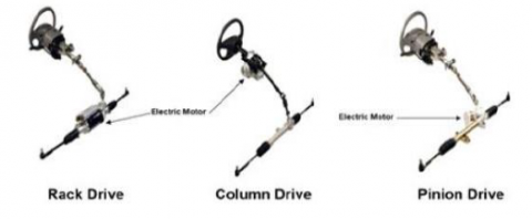
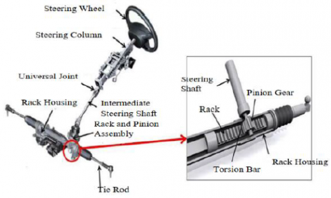
The steering system was widely used in the field of engineering; the most is automotive. Steering systems that use a lot of transmission mechanisms such as rack and pinion gear [1] as presented in Figure 1, steering systems with rack and gear type [2] as illustrated in Figure 2, steering systems with worm and sector type, steering systems with worm and tapered pin steering gear, steering system with worm and roller steering gear, steering system with recirculating ball type [3]. In 2009, Xu et al. [4] analyzed the stress and deformation of crown gear subjected to the heavy load in transmission condition between teeth. The investigation results outlined that the geometry of the tooth profile affected the contact conditions during gear transmission. In 2012, Rampilla [5] conducted a study using AutoCAD software and finite element methods to analyze and optimize Stress Intensity quantities and the obtained results are suitable size parameters using for fabrication, optimum bending stress, shape of gear, suitable for operation. In 2014, Xiao et al. [6] analyzed dynamic of gear and rack transmission system by using finite element analysis in ANSYS software. The results found the natural frequency of the gear transmission system, the optimal contact stress and bending stress of the gear and rack system. These help for selecting material and the geometry parameters of gear and rack to improve their durability. Shariff et al. [7] used transient dynamic and static analysis in ANSYS to determine deformation and stress of gear and rack on steering system. The simulated results indicated that bending stress and surface stress of gear teeth are the main factors leading to gear failure. In 2013, Sarkar et al. [8] carried out to design and analysis of steering gear and intermediate shaft for manual rack and pinion steering system based on the finite element analysis in ANSYS. The analysis results estimated steering rack deflection and bending stresses. The life of the intermediate steering shaft in cycles and the factor of safety of the shaft were computed by fatigue analysis. In 2016, Agrawal et al. [9] designed and manufactured a manual rack and pinion steering system according to the requirement of the vehicle for better maneuverability. In 2017, Thin Zar Thein Hlaing designed and analyzed of steering gear and intermediate shaft for the manual rack and pinion steering by FEA in ANSYS [2]. In 2018, Ramesh [10] utilized static analysis and transient dynamics in ANSYS to calculate contact stress and bending stress of rack and pinion. The analysis result pointed out that the Nickel Aluminum Bronze alloy [11] is suitable for fabricating rack and pinion.
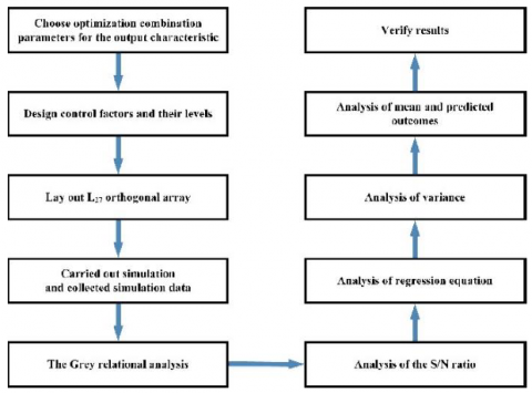
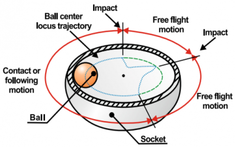
The clearance in the spherical joint and revolute joint makes the ball impact into the socket, and the journal impact into the bearing. The problem causes an impact on the mechanical systems, wear, and vibration. In other to reduce this problem, this study focuses on analyzing the influence of driven velocity, clearance of spherical and revolute joints, and coefficient of friction on the steering system based on the finite element method in ANSYS. The influence of design variables on maximum principal stress and strain helical gear and incline rack were minimized by grey relational analysis (GRA) based on Taguchi. The results of finite element analysis were verified by GRA, signal to noise (S/N) analysis, analysis of variance, mean analysis, regression analysis, interaction analysis, and surface analysis. The implementation steps have proceeded as depicted in Figure 3. Flowchart as shown in Figure 3, the research consists of 10 steps from designing of the model to simulation by ANSYS. Then use a variety of methods to increase the reliability of the output including the grey relational analysis, analysis of the S/N ratio, analysis of regression equation, analysis of mean, and finally verify results. The clearance model of the revolute joint, the spherical joint, and the designed mechanism setup of the finite element model and boundary condition are presented in Section 2. The Grey-Taguchi method is presented in Section 3. The outcomes and arguments will be presented in Section 4. The conclusions will be stated in Section 5.
Figure 1. The steering systems with rack and pinion gear [1]
Figure 2. steering systems model with rack and gear type [2]
Figure 3. Flow chart of research methodology
2.1 Designing the model in Solidworks and importing it to ANSYS
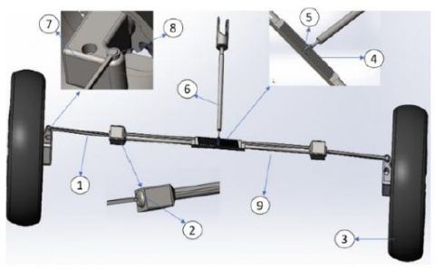
The model of the steering system used in this study is shown in Figure 4 including: Tie rod left and right (1), spherical joint (2), tire (3), incline rack (4), helical gear (5), gear shaft (6), steering arm (7) and revolute joint (8). The incline rack and helical gear of the steering system have a pinion, connected to the steering column. This pinion is connected to the steering tie rods. The pinion is helical gears. Helical gearing gives a smoother and quieter operation for the driver. Turning the steering wheel rotates the pinion, and moves the rack from side to side. Spherical joints at the end of the rack locate the tie-rods and allow movement in the steering and suspension. Mechanical advantage is gained by the reduction ratio. The value of this ratio depends on the size of the pinion. A small pinion gives light steering, but it requires many turns of the steering wheel.
Figure 4. Steering System with spherical joint, helical gear and incline rack
The geometrical parameters of the helical gear and incline rack were listed in Table 1. The Helical gear has 8 teeth, the helical angle is 40 degrees, the ring diameter is 15.665 mm and the module is 1.5. Helical gear is fitted with the incline rack that has 46 teeth, the incline angle is 15.4 degrees, and the same number of modules.
Table 1. The parameters of helical gear and rack
|
Helical Gear |
Rack |
||
|
Parameters |
Value |
Parameters |
Value |
|
Number of teeth |
8 |
Number of teeth |
46 |
|
Ring diameter (mm) |
15.665 |
Incline angle (degree) |
15.4 |
|
Outside diameter |
18,66 |
Modul (mm) |
1.5 |
|
Root diameter |
11,915 |
|
|
|
Helical angle (degree) |
40 |
|
|
|
Normal Modul (mm) |
1.5 |
|
|
|
Width (mm) |
35 |
|
|
2.2 Model of the revolute clearance joint
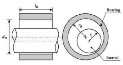
The center of the journal and the center of the bearing are concentric in the ideal joints but in the real joint is different. The clearance that exists in the real joint. The clearance size is the difference between the radius of the bearing and the radius of the journal and is determined by Eq. (1) [12-15]. The base connects to the crank due to the revolute joint with clearance as illustrated in Figure 5.
Figure 5. Revolute clearance joint model
$c=r_{b}-r_{j}$ (1)
where, rb, rj are the radii of the bearing and the journal, and lB and dB, are the length of bearing and diameter of the bearing, respectively.
2.3 Model of spherical clearance joint
The real spherical joint also exists the clearance and is determined the radius of socket minus the radius of ball [16-19]. Figure 6 is the spherical clearance joint links between inner tie rod and tie rod.
Figure 6. The model of spherical joint with clearance
2.4 Finite element model
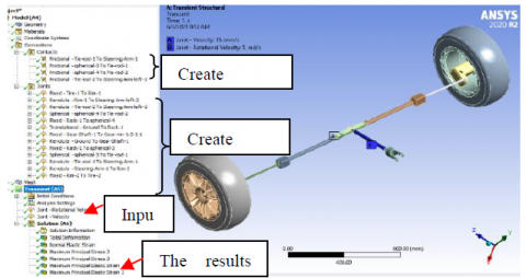
The finite element model of steering system and condition boundary was set up in ANSYS as depicted in Figure 7. The helical gear and rack were set flexible, the ball rigid, the socket is rigid, the helical gear is rotation, the rack drive linear motion. The material property of steering systems is structural steel with density is 7850 kg/m3, Young modulus of 200 GPa, Poisson’s ratio of 0.3. The steering system was divided meshing by automatic method with 42728 triangle elements and 182057 nodes. Firstly, this model has been created Contact between Tie-rod-1 to Steering-Arm-1, Spherical-3 to Tie-rod-1, Spherical-4 to Tie-rod-2 and Tie-rod-2 to steering Arm-left-2. Secondly, this model continually created the fix joint between Tie rod 1 and steering arm 1, spherical-3 and tie rod-1, spherical-4 and Tie-rod 2, Tie rod-2 and Steering Arm left-2. The joint between Tire-1 and Rim-1, Rack-1 and Spherical-4, Gear Shaft-1 and Gear-mn-1.5-1-1, Rack-1 and Spherical-3, Rim-2 and Tire 2 is Fixed. Rim-1 and Steering Arm Left-2, Tie rod 1 and Steering Arm 1, Steering Arm 1 and Rim 2 are revolute. The spherical-4 and Tie rod 2 are Spherical, and Ground and Rack-1 is Translational. Input velocity including Initial Condition, Analysis Settings, Joint-Rotational Velocity, Joint- Velocity. The result of the simulation pointed out solution Information, Normal Elastic Strain, Maximum Principal Stress 2, Maximum Principal Stress 3, Maximum Principal Elastic Strain, Maximum Principal Elastic Strain 2.
In this work, the coefficient friction in spherical joints and revolute joint are 0.01, 0.03 and 0.05, respectively. The simulation was performed assuming different clearance size spherical and revolute joint (c) with 0.01 mm, 0.1 mm and 1 mm. The driven speed was set up steering shaft is 5 rad/s, 7.5 rad/s, and 10 rad/s. The mechanical systems were simulayed in dry contact condition.
Figure 7. Modeling of finite element method in ANSYS
The Taguchi method based on grey relational analysis [20-29] was applied in this study to optimize these output characteristics.
Step 1: Choose optimization combination parameters for the output characteristics.
Step 2: Design control factors and their levels.
Step 3: Lay out L27 orthogonal array
Step 4: Carried out simulation and collected simulation data.
Step 5: The grey relational analysis (GRA) is a method to compare the changes of a system undergoing analysis to estimate the importance of design variable. The GRA is a method which applied to discretize sequences. GRA was carried out as follows.
Normalization: Rewrite each sequence between 0 and 1 as follows.
Larger the better mathematical formula:
$D_{i}^{*}=\frac{D_{i}^{(0)}(k)-\min D_{i}^{0}(k)}{\max D_{i}^{(0)}(k)-\min D_{i}^{(0)}(k)}$ (2)
Smaller the better:
$D_{i}^{*}=\frac{\max D_{i}^{(0)}(k)-D_{i}^{0}(k)}{\max D_{i}^{(0)}(k)-\min D_{i}^{(0)}(k)}$ (3)
Grey relational coefficient (GRC) (γ): is a quantity method in the grey relational space. GRC is required before determining the grey relational grade (GRG). The deviation is determined as follows:
${{\Delta }_{0i}}=\left\| D_{0}^{*}(k)-D_{i}^{*}k) \right\|$ (4)
${{\Delta }_{\min }}=\underset{\forall j\in i}{\mathop{\max }}\,\underset{\forall k}{\mathop{\min }}\,\left\| D_{0}^{*}(k)-D_{j}^{*}(k) \right\|$ (5)
${{\Delta }_{\max }}=\underset{\forall j\in i}{\mathop{\max }}\,\underset{\forall k}{\mathop{\max }}\,\left\| D_{0}^{*}(k)-D_{j}^{*}(k) \right\|$ (6)
Compute grey relational coefficient (GRC).
${{\gamma }_{i}}(k)=\frac{{{\Delta }_{\min }}+\xi {{\Delta }_{\max }}}{{{\Delta }_{0i}}+\xi .{{\Delta }_{\max }}}$ (7)
Here, $\xi \in[0,1]$ is the distinguishing coefficient, usually 0.5.
Compute GRG.
Determine the weight:
${{\omega }_{e}}(x)=x.{{e}^{(1-x)}}+(1-x){{e}^{x}}-1$ (8)
where, ωe(x) is the mapping function in entropy measurement and this function obtain maximum value when x=0.5 and e0.5-1=0.6487 and mapping value in [0,1] obtain as follow:
$w\equiv \frac{1}{({{e}^{0.5}}-1)}\sum\limits_{i=1}^{m}{{{\omega }_{e}}(x)}$
$\in =\{{{\gamma }_{i}}(1),\,\,{{\gamma }_{i}}(2),\,...,\,{{\gamma }_{i}}(n)\}.$ (9)
Note that, i=1, 2, ..., n.
Determine of the total of grey relational coefficient:
${{D}_{j}}\equiv \sum\limits_{i=1}^{m}{{{\gamma }_{i}}(j)},\,j=1,\,2,\,...,\,n$ (10)
Estimation of the normalized coefficient:
$k=\frac{1}{({{e}^{0.5}}-1)\times m}=\frac{1}{0.6487\times m}$ (11)
Determination of the entropy:
${{e}_{j}}=k\sum\limits_{i=1}^{m}{{{\omega }_{e}}}(\frac{{{\gamma }_{i}}(j)}{{{D}_{j}}}),\,j=1,\,2,\,...,\,n$ (12)
Here, ωe(x) uses Eq. (10).
Computation of sum of entropy:
$E=\sum\limits_{j=1}^{n}{{{e}_{j}}}$ (13)
Determination of the weight:
$\begin{align} & {{\omega }_{j}}=\frac{1}{n-E}.\frac{[1-{{e}_{j}}]}{\sum\limits_{j=1}^{n}{\frac{1}{n-E}.[1-{{e}_{j}}]}},\,\, \\ & \,\,\,\,\,\,\,\,\,\,\,\,\,\,\,\,\,\,\,\,here,\,j=1,\,2,\,...,\,n. \\\end{align}$ (14)
GRG (ψi) is the average value of GRC and written as follows:
${{\psi }_{i}}=\sum\limits_{k=1}^{n}{{{\omega }_{k}}{{\gamma }_{i}}}\left( k \right)$ (15)
where, n is the quantity of the experiment.
Step 6: Analysis of the S/N ratio.
“Larger is the better” approach [30-36]:
$S/N=-10\log (\frac{1}{n}\sum\limits_{i=1}^{n}{\frac{1}{y_{i}^{2}}})$ (16)
where, yi is the value measuring at ith simulation, n is the amount of simulation:
Step 7: Analysis of regression equation.
Step 8: Analysis of variance.
Step 9: Analysis of mean and predicted outcomes.
${{\mu }_{G}}={{G}_{m}}+\sum\limits_{i=1}^{q}{({{G}_{0}}}-{{G}_{m}})$ (17)
Step 10 verify results.
Besides, (CI) was also confirmed at the 95% confidence interval for both output characteristics and GRG by employing Eq. (18):
$C{{I}_{CE}}=\pm \sqrt{{{F}_{\alpha }}(1,fe)Ve(\frac{1}{{{n}_{eff}}}+\frac{1}{{{R}_{e}}}})$ (18)
Fα(1, fe) value look up in Table B-2, F-Table F0.05(f1,f2) as written of Ref. [37] at page 284.
4.1 Design simulation
Table 2. The designed variables and their levels
|
Factors |
|
Unit |
Levels |
||
|
1 |
2 |
3 |
|||
|
Clearance size |
A |
mm |
0.01 |
0.1 |
1 |
|
Friction Coefficient |
B |
0.01 |
0.03 |
0.05 |
|
|
Input rotation velocity |
C |
Rad/s |
5 |
7.5 |
10 |
Table 3. The L27 Orthogonal array and simulation results
|
Trial No. |
A |
B |
C |
Stress of Gear |
Stress of Rack |
|
1 |
0.01 |
0.01 |
5 |
0.1638 |
0.0188 |
|
2 |
0.01 |
0.01 |
7.5 |
0.1841 |
0.0281 |
|
3 |
0.01 |
0.01 |
10 |
0.1921 |
0.0371 |
|
4 |
0.01 |
0.03 |
5 |
0.1449 |
0.0191 |
|
5 |
0.01 |
0.03 |
7.5 |
0.2667 |
0.0283 |
|
6 |
0.01 |
0.03 |
10 |
0.3728 |
0.0372 |
|
7 |
0.01 |
0.05 |
5 |
0.1735 |
0.0193 |
|
8 |
0.01 |
0.05 |
7.5 |
0.2288 |
0.0285 |
|
9 |
0.01 |
0.05 |
10 |
0.3708 |
0.0375 |
|
10 |
0.1 |
0.01 |
5 |
0.1675 |
0.0195 |
|
11 |
0.1 |
0.01 |
7.5 |
0.2498 |
0.0287 |
|
12 |
0.1 |
0.01 |
10 |
0.3836 |
0.0379 |
|
13 |
0.1 |
0.03 |
5 |
0.1953 |
0.0197 |
|
14 |
0.1 |
0.03 |
7.5 |
0.2089 |
0.0282 |
|
15 |
0.1 |
0.03 |
10 |
0.3344 |
0.0381 |
|
16 |
0.1 |
0.05 |
5 |
0.2182 |
0.0221 |
|
17 |
0.1 |
0.05 |
7.5 |
0.3231 |
0.0375 |
|
18 |
0.1 |
0.05 |
10 |
0.4261 |
0.0383 |
|
19 |
1 |
0.01 |
5 |
0.2121 |
0.0203 |
|
20 |
1 |
0.01 |
7.5 |
0.2635 |
0.0289 |
|
21 |
1 |
0.01 |
10 |
0.3374 |
0.0385 |
|
22 |
1 |
0.03 |
5 |
0.2205 |
0.0223 |
|
23 |
1 |
0.03 |
7.5 |
0.2739 |
0.0291 |
|
24 |
1 |
0.03 |
10 |
0.3575 |
0.0387 |
|
25 |
1 |
0.05 |
5 |
0.2783 |
0.0204 |
|
26 |
1 |
0.05 |
7.5 |
0.3643 |
0.0293 |
|
27 |
1 |
0.05 |
10 |
0.4374 |
0.0389 |
The input variables and their levels in this study are shown in Table 2. First, A is the symbol of clearance size with 3 levels respectively 0.01, 0.1, and 1, unit mm. Second, the friction coefficient is B with 3 levels respectively 0.01, 0.03, 0.05, and this variable has no unit and finally Input rotation velocity is denoted by C, unit 3 levels respectively as follows: 5 Rad/s, 7.5 Rad/s, 10 Rad/s.
After using Minitab 18 software and based on the designed variables in Table 3, this study has divided 27 cases that are completely different for simulation purposes. All of them are presented in Table 3. The results of stress simulation of helical gear and rack are also shown in that table. According to this Table, the increase of Clearance size (A) leads to an increase in the stress variable, but not much. Similarly, the friction coefficient (B) increases and also causes the stress to increase not much. However, the Input rotation velocity (C) has a strong influence on stress.
4.2 Grey relational analysis
$D_{i}^{*}(1)$ and $D_{i}^{*}(2)$ are objective functions. In order for the steering mechanism to work optimally, the stress of the helical gear and rack should be as small as possible so equation number Eq. (3) is applied to minimize the stress. The results are shown in Table 3. ∆oi(1) and ∆oi(2) are the deviation values of strain and stress, respectively obtained by Eq. (3). gi(1) and gi(2) are the GRC of the deviation response of displacement and stress, respectively obtained by equation (6), GRG (yi) is calculated by Eq. (14), and Rank are cases sorted by optimality. And the last column in the table shows the results of the signal-to-noise (S/N) analysis. In this Table, the min value of ∆oi is zero and the max value of ∆oi is one. From Table 4, this study obtains the max and min values corresponding to the 16th test and the 4th test, respectively.
4.3 Analysis of signal to noise
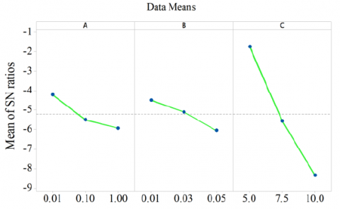
The chart of the SN ratio is shown in Figure 8. It shows the change of individual response of three variables which are clearance size (A), friction coefficient (B), and input rotation velocity (C). In the graph, the x-axis represents the value of each process parameter and the y-axis is the response value. The horizontal line shows the average value of the response. Key effects tiles are used to define optimal design conditions for optimum strain and stress of helical gear and incline rack. The maximum value shown in the graph is the optimal level, so the optimal level of the combined variable here is A1B1C1. The steeper the graph of the variables, the more it affects the output, so variable C has the greatest influence on the stress of the rack and pinion, then variable A, and finally variable B.
The mean of signal to noise each variable at each level is presented in Table 5. The delta is calculated by the maximum value minus the minimum value of S/N in the 2nd column for variable A, the 3rd column for variable B and the 4th column for variable C.
Figure 8. Main effects plot for SN ratios
Table 4. The smaller the better of S/N value deviation, GRC, GRG and rank of GRG
|
Trial No. |
$D_{i}^{*}$ (1) |
$D_{i}^{*}$ (2) |
Δoi(1) |
Δoi(2) |
γi(1) |
γi(2) |
ψi |
Rank |
S/N of GRG |
|
1 |
0.9354 |
1.0000 |
0.0646 |
0.0000 |
0.8856 |
1.0000 |
0.9430 |
2 |
-0.5098 |
|
2 |
0.8660 |
0.5373 |
0.1340 |
0.4627 |
0.7886 |
0.5194 |
0.6535 |
10 |
-3.6951 |
|
3 |
0.8386 |
0.0896 |
0.1614 |
0.9104 |
0.7560 |
0.3545 |
0.5545 |
13 |
-5.122 |
|
4 |
1.0000 |
0.9851 |
0.0000 |
0.0149 |
1.0000 |
0.9711 |
0.9855 |
1 |
-0.1269 |
|
5 |
0.5836 |
0.5274 |
0.4164 |
0.4726 |
0.5456 |
0.5141 |
0.5298 |
15 |
-5.5178 |
|
6 |
0.2209 |
0.0846 |
0.7791 |
0.9154 |
0.3909 |
0.3533 |
0.3720 |
22 |
-8.5891 |
|
7 |
0.9022 |
0.9751 |
0.0978 |
0.0249 |
0.8364 |
0.9526 |
0.8947 |
4 |
-0.9665 |
|
8 |
0.7132 |
0.5174 |
0.2868 |
0.4826 |
0.6355 |
0.5089 |
0.5720 |
12 |
-4.8521 |
|
9 |
0.2277 |
0.0697 |
0.7723 |
0.9303 |
0.3930 |
0.3496 |
0.3712 |
24 |
-8.6078 |
|
10 |
0.9227 |
0.9652 |
0.0773 |
0.0348 |
0.8661 |
0.9349 |
0.9006 |
3 |
-0.9094 |
|
11 |
0.6414 |
0.5075 |
0.3586 |
0.4925 |
0.5823 |
0.5038 |
0.5429 |
14 |
-5.3056 |
|
12 |
0.1839 |
0.0498 |
0.8161 |
0.9502 |
0.3799 |
0.3448 |
0.3623 |
25 |
-8.8186 |
|
13 |
0.8277 |
0.9552 |
0.1723 |
0.0448 |
0.7437 |
0.9178 |
0.8311 |
5 |
-1.6069 |
|
14 |
0.7812 |
0.5323 |
0.2188 |
0.4677 |
0.6956 |
0.5167 |
0.6058 |
11 |
-4.3534 |
|
15 |
0.3521 |
0.0398 |
0.6479 |
0.9602 |
0.4356 |
0.3424 |
0.3888 |
20 |
-8.2055 |
|
16 |
0.7494 |
0.8358 |
0.2506 |
0.1642 |
0.6661 |
0.7528 |
0.7096 |
7 |
-2.9797 |
|
17 |
0.3908 |
0.0697 |
0.6092 |
0.9303 |
0.4508 |
0.3496 |
0.4000 |
19 |
-7.9588 |
|
18 |
0.0386 |
0.0299 |
0.9614 |
0.9701 |
0.3421 |
0.3401 |
0.3411 |
26 |
-9.3424 |
|
19 |
0.7703 |
0.9254 |
0.2297 |
0.0746 |
0.6852 |
0.8702 |
0.7781 |
6 |
-2.1793 |
|
20 |
0.5945 |
0.4975 |
0.4055 |
0.5025 |
0.5522 |
0.4988 |
0.5254 |
16 |
-5.5902 |
|
21 |
0.3419 |
0.0199 |
0.6581 |
0.9801 |
0.4317 |
0.3378 |
0.3846 |
21 |
-8.2998 |
|
22 |
0.7415 |
0.8259 |
0.2585 |
0.1741 |
0.6592 |
0.7417 |
0.7006 |
8 |
-3.0906 |
|
23 |
0.5590 |
0.4876 |
0.441 |
0.5124 |
0.5313 |
0.4939 |
0.5125 |
17 |
-5.8061 |
|
24 |
0.2732 |
0.0100 |
0.7268 |
0.9900 |
0.4076 |
0.3356 |
0.3715 |
23 |
-8.6008 |
|
25 |
0.5439 |
0.9204 |
0.4561 |
0.0796 |
0.5230 |
0.8627 |
0.6935 |
9 |
-3.1791 |
|
26 |
0.2499 |
0.4776 |
0.7501 |
0.5224 |
0.4000 |
0.489 |
0.4447 |
18 |
-7.0387 |
|
27 |
0.0000 |
0.0000 |
1.0000 |
1.0000 |
0.3333 |
0.3333 |
0.3333 |
27 |
-9.5433 |
Table 5. Response table for signal to noise ratios
|
Level |
A |
B |
C |
|
1 |
-4.221 |
-4.492 |
-1.728 |
|
2 |
-5.498 |
-5.100 |
-5.569 |
|
3 |
-5.925 |
-6.052 |
-8.348 |
|
Delta |
1.705 |
1.560 |
6.620 |
|
Rank |
2 |
3 |
1 |
4.4 Analysis of mean
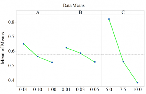
The graph’s main effects plot for means was shown in Figure 9. It identified that the change in the individual reaction of three variables A, B, and C. In the graph, the x-axis represents the level of each variable and the y-axis is the mean of means. The high peaks of the graph determined the optimal value of the design variable. Therefore, the optimal level of the combined variable is A1B1C1. The mean of the main effects plot for the mean of each variable at each level is presented in Table 6 below. The delta is calculated by the maximum value minus the minimum value of S/N in the 2nd column for variable A, the 3rd column for variable B and the 4th column for variable C.
Table 6. Response table for means of GRG
|
Level |
A |
B |
C |
|
1 |
0.6529 |
0.6272 |
0.8263 |
|
2 |
0.5647 |
0.5886 |
0.5318 |
|
3 |
0.5271 |
0.5289 |
0.3866 |
|
Delta |
0.1258 |
0.0983 |
0.4397 |
|
Rank |
2 |
3 |
1 |
Figure 9. The graph of the main effects plots for the mean
4.5 Analysis of interaction
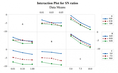
As depicted in Figure 10, the interaction between the design variables and pointed out effects of the design variables the S/N of GRG. The design variables have interaction when the graph is the non-parallel lines and effected significantly on the S/N of GRG values. When the graph is parallel lines, the design variables haven’t interacted with each other, thereby the design variables slightly effected on the S/N of GRG values.
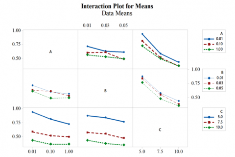
As presented in Figure 11, the interaction between the design variables and pointed out effects of the design variables the means of GRG. The design variables have interaction when the graph is the non-parallel lines and effected significantly on the means of GRG values. When the graph is parallel lines, the design variables haven’t interacted with each other, thereby the design variables slightly effected on the means of GRG values. The problem shows that the choice of design variables is very important and cannot be ignored.
Figure 10. The graph of the interaction for signal to noise
Figure 11. The graph of interaction for mean
4.6 Analysis of variance
The ANOVA for output responses is listed in Table 7 namely the degree of freedom, a sum of the square, contribution percent, mean square, F-value and P-value of the regression equation, single factor, interaction factor, error, and total. The contribution percent of the regression equation is 95.67%, the contribution percent of A is 4.26%, B is 4.01%, C is 80.28%, A*A is 2.67%, A*C is 1.37%, C*C is 9.63%, the error is 4.33%. The mean square of the regression equation is 0.172809, A is 0.046117, B is 0.043493, C is 0.870056, C*C is 0.033391, A*A is 0.028924, A*C is 0.028924 and the error is 0.002347. The P-value reveals that the input parameters are significant, as the P-value is less than 0.05. The ANOVA analysis results agree well with the signal-to-noise analysis results. It means that variable c has the most influence on variable A and finally variable B.
Table 8 was pointed out R-sq is 98.81%, R-sq(adj) is 98.60%, R-sq(pred) is 98.41%.
Table 7. The outline of the analysis of variance
|
Source |
DF |
Seq SS |
Contribution |
Adj SS |
Seq MS |
F-Value |
P-Value |
|
Regression |
6 |
1.03685 |
95.67% |
1.03685 |
0.172809 |
73.63 |
0.000 |
|
A |
1 |
0.04612 |
4.26% |
0.04445 |
0.046117 |
19.65 |
0.000 |
|
B |
1 |
0.04349 |
4.01% |
0.04349 |
0.043493 |
18.53 |
0.000 |
|
C |
1 |
0.87006 |
80.28% |
0.07841 |
0.870056 |
370.72 |
0.000 |
|
A*A |
1 |
0.02892 |
2.67% |
0.02892 |
0.028924 |
12.32 |
0.002 |
|
C*C |
1 |
0.03339 |
3.08% |
0.03339 |
0.033391 |
14.23 |
0.001 |
|
A*C |
1 |
0.01487 |
1.37% |
0.01487 |
0.014872 |
6.34 |
0.020 |
|
Error |
20 |
0.04694 |
4.33% |
0.04694 |
0.002347 |
||
|
Total |
26 |
1.08379 |
100% |
Table 8. Model summary for transformed response
|
S |
R-sq |
R-sq(adj) |
PRESS |
R-sq(pred) |
|
0.0484450 |
95.67% |
94.37% |
0.0803578 |
92.59% |
4.7 Regression equation
The GRG regression equation is obtained as written in Eq. (19). From this equation, the predicted value of GRG obtained with the combined parameters A1B1C1 is 0.97. The optimal value of GRG is 0.943, the error between the predicted value and the optimal value is 2.79%. Residual Plot for GRG as shown in Figure 12 demonstrated the data of the simulation lies near the straight line with an error in the interval [-0.08, 0.08].
$\begin{align} & GRG=0.948{{A}^{2}}+0.01194{{C}^{2}}+0.0257AC \\ & \,\,\,\,\,\,\,\,\,\,\,\,\,\,\,\,\,\,\,\,-1.277A-2.458B-0.2765C+2.09 \\\end{align}$ (19)
Figure 12. Residual plots for GRG
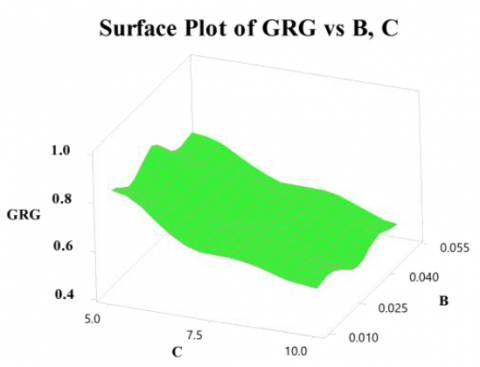
4.8 Analysis of surface plot
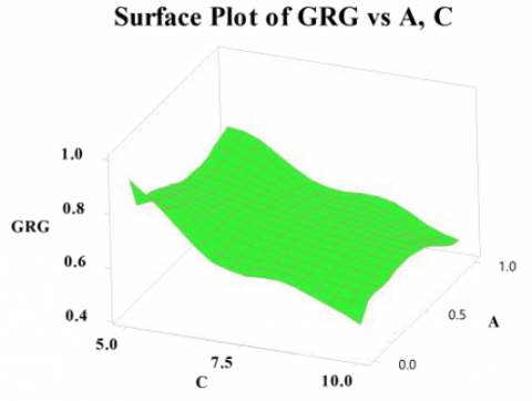
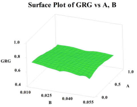
The surface plot of GRG as depicted in Figure 13a did not change significantly as B increased gradually. The value of GRG changed significantly as C decreased. From there, it showed that the input speed increased to make the strain and stress of the helical gear and rack of the steering system increased. In Figure 13b the value of GRG changed significantly as C decreased and almost did not change as an increased. From there, it showed that the input friction coefficient increased, causing the tension and stress of the helical gear and rack to change. As can be seen in Figure 13c The GRG value is almost unchanged as A and B increase gradually.
a) Surface plot of GRG vs B, C
b) Surface plot of GRG vs A, C
c) Surface plot of GRG vs A, B
Figure 13. Surface plot of GRG
At 95% confidence interval (CI) and presented in predictive optimization. The result of optimization of GRG is 0.943, the predicted value of GRG is 0.9432, the deviation between the predicted and optimal value is 0.022%.
$\begin{align} & {{\mu }_{G}}={{G}_{m}}+\sum\limits_{i=1}^{q}{({{G}_{0}}}-{{G}_{m}})=A1+B1+C1-2\times {{G}_{m}} \\ & \,\,\,\,\,\,\,\,\,=0.6529+0.6272+0.8263-2\times 0.5816=0.9432 \\\end{align}$
For GRG, at a=0.05, fe=20, F0.05(1,20)=4.3513, Ve=0.002347 [37], R=4, Re=1, n=27.
$C{{I}_{CE}}=\pm \sqrt{4.3513\times 0.002345\times (\frac{1}{\frac{27}{1+7}}+1)}=\pm 0.115$
$0.8282<{{\mu }_{confirmation}}<1.0582$
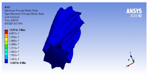
The optimum stress value and the maximum principal elastic strain as shown in Figure 14, and Figure 15 are 0.16382 MPa and 7.6761e-7 mm/mm. This result is better than in Ramesh R.'s experiment [10, 11].
Figure 14. The optimal result of maximum principle stress of gear
Figure 15. Elastic strain of gear
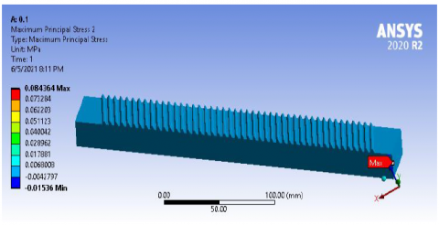
Figure 16. Maximum principal stress of rack
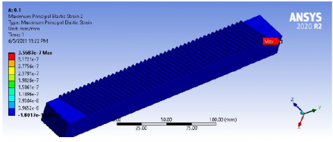
Figure 17. Maximum principal elastic strain of rack
In Figure 16 and Figure 17, the optimal maximum principal stress of rack and the maximum principal elastic strain of rack at the level of 0.084364 MPa and 3.5687e-7 mm/mm. The outcome of this study which is more optimal than this investigation [10, 11].
This investigation presented and discussed how to optimize the strain and stress of gear and racks on the steering system. Taguchi with grey relational analysis was used in this research. The simulation results demonstrated that the design variables affected on strain and stress of helical gear and rack. The problem is verified by the grey relational analysis based on Taguchi method, ANOVA, and analysis signal to noise. The nonlinear regression was applied to optimize the design strain and stress of helical gear and rack. First, the effects of clearance size of spherical and revolute joint, friction, and input velocity on the steering mechanism were analyzed by ANSYS. Up to now, there were no investigations have used ANSYS to analyze these effects. Therefore, this is the first time that ANSYS has been applied to calculate the strain and stress of the rack and helical gear of the steering system. To do this work, firstly the studying model was designed by Solidworks. the Taguchi method. The goals of this research are to increase the endurance of the elements, reduce maintenance costs due to joint wear, and save time and money. Second, the Grey relational analysis based on the Taguchi method is also used to select results with minimum stress and strain. The regression analysis and ANOVA have small deviations from the results of FEM. Third, the results of surface plot analysis are close to the FEM. Finally, computational methods and research have shown that Grey based on Taguchi has adopted multi-objective optimization to apply strict adherence mechanisms and optimal design with deviation error from the results of the simulation. The optimal results of the stress of gear and rack have been achieved at 0.1638 MPa and 0.0188 MPa, respectively. The simulation results revealed that the input rotation velocity (C) significantly affected the stress of gear and rack, followed by the variable clearance size (A) and finally the variable friction coefficient(B). This is also confirmed grey relational analysis based on the Taguchi method, analysis of the signal to noise, analysis of variance (ANOVA), regression analysis, and analysis of surface plot.
[1] Khan, I.R., Shrikant, B.R., Choudhary, F., Jadhav, R., Shirbhate, S. (2019). Front wheel steering system & adaptability of rack and pinion steering over the other steering systems. International Journal for Research & Development in Technology, 7(2): 229-231. https://www.researchgate.net/publication/330882189
[2] Hlaing, T.Z.T., Win, H., Thein, M. (2017). Design and analysis of steering gear and intermediate shaft for manual rack and pinion steering system. International Journal of Scientific and Research Publications, 7(12): 861-882. http://www.ijsrp.org/research-paper-1217/ijsrp-p72108.
[3] Popa, C.E. (2005). Steering system and suspension design for 2005 Formula SAE-A Racer Car. University of Southern Queensland, Faculty of Engineering and Surveying, 1-120. https://eprints.usq.edu.au/530/1/CristinaelenaPOPA-2005.
[4] Xu, L., Li, L., Liu, Y. (2009). Stress analysis and optimization of gear teeth. International Conference on Measuring Technology and Mechatronics Automation, pp. 895-898. https://doi.org/10.1109/ICMTMA.2009.610
[5] Rampilla, L.S.M. (2012). A finite element approach to stress analysis of face gears. Cleveland State University, 1-54. https://engagedscholarship.csuohio.edu/cgi/viewcontent.cgi?article=1636&context=etdarchive.
[6] Xiao, Y.J., He, L.H., Zhu, J.Y., Xiao, Y.C. (2014). Dynamic analysis of gear and rack transmission system. The Open Mechanical Engineering Journal, 8(1): 662-667. http://dx.doi.org/10.2174/1874155X01408010662
[7] Shariff, S., Nagaraju, K., Praveen. (2018). Analysis of gear and rack transmission system. Department of Mechanical Engineering Sreenidhi Institute of Science & Technology, 1-24.
[8] Sarkar, G.T., Yenarkar, Y.L., Bhope, D.V. (2013). Stress analysis of helical gear by finite element method. International Journal of Mechanical Engineering and Robotics Research, 2(4): 322-329. http://www.ijmerr.com/v2n4/ijmerr_v2n4_39.
[9] Agrawal, P.L., Patel, S.S., Parmar, S.R. (2016). Design and simulation of manual rack and pinion steering system. International Journal for Science and Research Technology (IJSART), 2(7): 1-4.
[10] Ramesh, R. (2018). Static and transient analysis of Rack and Pinon. International Journal of Research in Mechanical, Mechatronics and Automobile Engineering. 4(2): 45-50. http://www.ijrmmae.in/Volume4-Issue-2/paper8.
[11] Xiao, Y.J., He, L.H., Zhu, J.Y., Xiao, Y.C. (2014). Dynamic analysis of gear and rack transmission system. The Open Mechanical Engineering Journal, 8(1): 662-667. http://dx.doi.org/10.2174/1874155X01408010662
[12] Mukras, S., Kim, N.H., Mauntler, N.A., Schmitz, T., Sawyer, W.G. (2010) Comparison between elastic foundation and contact force models in wear analysis of planar multibody system. Journal of Tribology, 132(3): 1-11. https://doi.org/10.1115/1.4001786
[13] Tian, Q., Liu, C., Machado, M., Flores, P. (2011). A new model for dry and lubricated cylindrical joints with clearance in spatial flexible multibody systems. Nonlinear Dynamics, 64(1): 25-47. https://doi.org/10.1007/s11071-010-9843-y
[14] Koshy, C.S., Flores, P., Lankarani, H.M. (2013). Study of the effect of contact force model on the dynamic response of mechanical systems with dry clearance joints: computational and experimental approaches. Nonlinear Dynamics, 73(1): 325-338. https://doi.org/10.1007/s11071-013-0787-x
[15] Meng, F., Wu, S., Zhang, F., Zhang, Z., Hu, J., Li, X. (2015). Modeling and simulation of flexible transmission mechanism with multiclearance joints for ultrahigh voltage circuit breakers. Shock and Vibration, 2015: 1-17. https://doi.org/10.1155/2015/392328
[16] Zheng, E., Zhu, R., Zhu, S., Lu, X. (2016). A study on dynamics of flexible multi-link mechanism including joints with clearance and lubrication for ultra-precision presses. Nonlinear Dynamics, 83(1): 137-159. https://doi.org/10.1007/s11071-015-2315-7
[17] Erkaya, S., Doğan, S., Şefkatlıoğlu, E. (2016). Analysis of the joint clearance effects on a compliant spatial mechanism. Mechanism and Machine Theory, 104: 255-273. https://doi.org/10.1016/j.mechmachtheory.2016.06.009
[18] Flores, P., Lankarani, H.M. (2010). Spatial rigid-multibody systems with lubricated spherical clearance joints: modeling and simulation. Nonlinear Dynamics, 60(1): 99-114. https://doi.org/10.1007/s11071-009-9583-z
[19] Ambrósio, J., Verissimo, P. (2009). Improved bushing models for general multibody systems and vehicle dynamics. Multibody System Dynamics, 22(4): 341-365. https://doi.org/10.1007/s11044-009-9161-7
[20] Hoang, V.H., Huynh, N.T., Nguyen, H., Huang, S.C. (2019). Analysis and optimal design a new flexible hinge displacement amplifier mechanism by using Finite element analysis based on Taguchi method. In 2019 IEEE Eurasia Conference on IOT, Communication and Engineering (ECICE), pp. 259-262. https://doi/10.1109/ECICE47484.2019.8942671
[21] Huynh, N.T., Huang, S.C., Dao, T.P. (2021). Optimal displacement amplification ratio of bridge-type compliant mechanism flexure hinge using the Taguchi method with grey relational analysis. Microsystem Technologies, 27(4): 1251-1265. https://doi.org/10.1007/s00542-018-4202-x
[22] Huynh, N.T., Huang, S.C., Dao, T.P. (2020). Design variables optimization effects on acceleration and contact force of the double sliders-crank mechanism having multiple revolute clearance joints by use of the Taguchi method based on a grey relational analysis. Sādhanā, 45(1): 1-22. https://doi.org/10.1007/s12046-020-01346-w
[23] Vu, N.C., Huynh, N.T., Huang, S.C. (2019). Optimization the first frequency modal shape of a tensural displacement amplifier employing flexure hinge by using Taguchi Method. In Journal of Physics: Conference Series, 1303(1): 012016. https://doi.org/10.1088/1742-6596/1303/1/012016
[24] Wang, C.N., Truong, K.P., Huynh, N.T., Nguyen, H. (2019). Optimization on effects of design parameter on displacement amplification ratio of 2 DOF working platform employing Bridge-type compliant mechanism flexure hinge using Taguchi method. In Journal of Physics: Conference Series, 1303(1): 012053. https://doi.org/10.1088/1742-6596/1303/1/012053
[25] Wang, C.N., Truong, K.P., Huynh, N.T. (2019). Optimization effects of design parameter on the first frequency modal of a Bridge-type compliant mechanism flexure hinge by using the Taguchi method. In Journal of Physics: Conference Series, 1303(1): 012063. https://doi.org/10.1088/1742-6596/1303/1/012063
[26] Tran, Q.P., Huynh, N.T., Huang, S.C. (2021). Artificial neural network base on grey relational analysis estimate displacement of bridge-type amplifier. In IOP Conference Series: Materials Science and Engineering, 1113(1): 012007. https://doi.org/10.1088/1757-899X/1113/1/012007
[27] Ghani, J.A., Choudhury, I.A., Hassan, H.H. (2004). Application of Taguchi method in the optimization of end milling parameters. Journal of Materials Processing Technology, 145(1): 84-92. https://doi.org/10.1016/S0924-0136(03)00865-3
[28] Jung J.H., Kwon, W.T. (2010). Optimization of EDM process for multiple performance characteristics using Taguchi method and Grey relational analysis. Journal of Mechanical Science and Technology, 24: 1083-1090. 2010. https://doi.org/10.1007/s12206-010-0305-8
[29] Huynh N.T., Nguyen, Q.M. (2021). Application of grey relational approach and artificial neural network to optimise design parameters of bridge-type compliant mechanism flexure hinge. International Journal of Automotive and Mechanical Engineering, 18(1): 8505-8522. htps://doi.org/10.15282/ijame.18.1.2021.10.0645
[30] Nalbant, M., Gökkaya, H., Sur, G. (2007). Application of Taguchi method in the optimization of cutting parameters for surface roughness in turning. Materials & Design, 28(4): 1379-1385. https://doi.org/10.1016/j.matdes.2006.01.008
[31] Asiltürk, I., Neşeli, S., Ince, M.A. (2016). Optimisation of parameters affecting surface roughness of Co28Cr6Mo medical material during CNC lathe machining by using the Taguchi and RSM methods. Measurement, 78: 120-128. https://doi.org/10.1016/j.measurement.2015.09.052
[32] Aber, S., Salari, D., Parsa, M.R. (2010). Employing the Taguchi method to obtain the optimum conditions of coagulation–flocculation process in tannery wastewater treatment. Chemical Engineering Journal, 162(1): 127-134. https://doi.org/10.1016/j.cej.2010.05.012
[33] Chen, W.C., Hsu, Y.Y., Hsieh, L.F., Tai, P.H. (2010). A systematic optimization approach for assembly sequence planning using Taguchi method, DOE, and BPNN. Expert Systems with Applications, 37(1): 716-726. https://doi.org/10.1016/j.eswa.2009.05.098
[34] Liu, Y.T., Chang, W.C., Yamagata, Y. (2010), A study on optimal compensation cutting for an aspheric surface using the Taguchi method. CIRP Journal of Manufacturing Science and Technology, 3(1): 40-48. https://doi.org/10.1016/j.cirpj.2010.03.001
[35] Sarıkaya, M., Güllü, A. (2015) Multi-response optimization of minimum quantity lubrication parameters using Taguchi-based grey relational analysis in turning of difficult-to-cut alloy Haynes 25. Journal of Cleaner Production, 91: 347-357. https://doi.org/10.1016/j.jclepro.2014.12.020
[36] Deepanraj, B., Sivasubramanian, V., Jayaraj, S. (2017). Multi-response optimization of process parameters in biogas production from food waste using Taguchi – Grey relational analysis. Energy Conversion and Management. 141: 429-438. https://doi.org/10.1016/j.enconman.2016.12.013
[37] Roy, R.K. (2010). A primer on the Taguchi method, 2nd edition. The United States of American.