Syamsul Amar![]() | Alpon Satrianto
| Alpon Satrianto![]() | Ariusni
| Ariusni![]() | Anggi Putri Kurniadi*
| Anggi Putri Kurniadi*![]()
© 2023 IIETA. This article is published by IIETA and is licensed under the CC BY 4.0 license (http://creativecommons.org/licenses/by/4.0/).
OPEN ACCESS
This study aims to analyze the shock response between the variables of economic growth, consumption, investment, government spending, export, poverty, unemployment and income inequality in all provinces in Indonesia during 2015-2021. This research is important because promoting economic stability is a major goal of economic policy and allows other macroeconomic goals to be achieved. The novelty of this study is to analyze shocks to macroeconomic variables consisting of economic growth, fiscal indicators, monetary indicators and welfare indicators by using the Panel Vector Autoregression (PVAR). The results of the study conclude that there is a causal relationship between unemployment and export; unemployment and poverty; poverty and export; unemployment and poverty. Furthermore, variables that have a one-way relationship such as economic growth affect consumption; consumption affects government spending; government spending affects investment; investment affects export. The recommendations from this study require that the government must be proactive in encouraging other elements, such as the private sector, which has a big role in helping government programs run optimally. The limitation of this research is the research methodology because all the research variables are endogenous and only analyze balance in the long run.
macroeconomics, response, shock
The economic system tends to create linkages between macroeconomic variables [1-6]. The linkages between macroeconomic variables will lead to balance and can impact people's welfare [7-15]. Concretely, if one of the variables experiences a shock, the other economic variables will also respond. For example, when there is a decline in economic growth, this condition will be responded to by increasing unemployment, poverty, income distribution inequality, and so on. On the other hand, an increase in the decline in investment will be responded to by a decrease in economic growth, weakening consumption, and increasing poverty.
The level of response to changes that occur in a macroeconomic variable as a result of a change in a macro variable is determined by the level of sensitivity of the macroeconomic variable and the existing economic conditions. At that time, it has the potential to cause shocks to other macro variables [16-22]. The level of shocks tends to trigger an imbalance in an economic system which must be followed up with effective policies so that the economy is always in balance [23, 24].
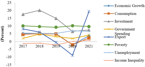
Based on the background of the empirical phenomena described, this condition is in line with the factual phenomena that have occurred in Indonesia in the last five years, which as a developing country, tends to experience shocks to macroeconomic variables. Conditions for the growth of various macroeconomic variables in Indonesia can be seen in Figure 1.
The information obtained from Figure 1 shows that macroeconomic variables in Indonesia tend to experience shocks due to fluctuations every year. However, the focus of attention on several macroeconomic variables in Figure 1 is the trend of economic growth because economic growth serves as a benchmark for the success or decline of a country's economy and an indicator of people's welfare. When economic growth experiences shock, there are various unstable economic indicators. The condition of economic growth in Indonesia during the period 2017 to 2020 tends to experience a negative trend, while conditions will contrast in 2021.
Figure 1. Growth conditions of various macroeconomic variables in Indonesia [25]
Economic growth in Indonesia experienced a slight decline of 0.02 points in 2018 of 5.17 percent compared to 2017 of 5.19 percent. This condition was caused by increasing global uncertainty from the external sector, both from the trade channel and the financial channel. From the trade channel, export performance declined due to slowing world economic growth and falling commodity prices. Moreover, the challenges from the trade channel are getting stronger because, at the same time, the demand for imports for domestic infrastructure projects is quite large. Meanwhile, the challenge from the financial channel is the reduced inflow of foreign capital to developing countries, including Indonesia, due to the increase in the US monetary policy rate and uncertainty in global financial markets.
Furthermore, economic growth in Indonesia decreased again by 0.10 points in 2019 by 5.07 percent compared to 2018. This condition was caused by structural shifts in the global economy, which had an impact on weakening world economic growth, posing challenges to the 2019 domestic economy. The economy in 2019 was not as strong as the previous year's growth, although it remained resilient, supported by good domestic demand and maintained stability.
Then, economic growth in Indonesia decreased sharply by 3 points in 2020 by -2.07 percent compared to 2019. This condition occurred because the Corona Virus Disease 2019 (COVID-19) pandemic had an extraordinary influence on the dynamics of the world economy in 2020, including Indonesia. COVID-19 spread to nearly 178 countries worldwide and infected more than 85 million people, bringing more than 1.8 million deaths in 2020. This condition created a health and humanitarian crisis, an economic crisis, and increased poverty. In addition, various macroeconomic indicators pointed to sharp pressures on consumption, investment, and production activities, resulting in a decline in international trade.
Different conditions for economic growth in Indonesia in 2021 amounted to 3.69 percent, which has increased by 1.62 points compared to 2020. This condition occurs because the process of national economic recovery continues with stability being maintained. However, the process of recovering the domestic economy in 2021 will still be affected by the continuation of the COVID-19 pandemic. In addition, the outbreak of the COVID-19 variant of the Delta in the third quarter of 2021 is holding back the process of Indonesia's economic recovery. Nevertheless, economic performance is predicted to increase in the fourth quarter of 2021, supported by mobility that continues to increase in line with the acceleration of vaccination and the waning spread of COVID-19, the opening up of broader economic sectors, continuing policy stimulus, and export performance that remains strong.
Based on this explanation, this study will examine macroeconomic variable shocks in Indonesia. This is important because a balanced economy is related to macroeconomic stability, which occurs when macroeconomic indicators move in a favorable direction and do not change much over time. Promoting economic stability in a country is a key objective of economic policy because economic stability allows other macroeconomic objectives to be achieved, such as stable prices and sustainable growth, creating the right environment for increased employment and balance of payments. In addition, macroeconomic stability is important in making economic decisions because it makes it easier for businesses to predict economic indicators. Conversely, instability can increase uncertainty, hinder investment, hamper economic growth, and reduce people's living standards. The novelty of this study is to analyze shocks to macroeconomic variables consisting of the economic growth, fiscal indicators (government spending), monetary indicators (investment and export) and welfare indicators (consumption, poverty, unemployment and income inequality). The structure of the description of this article for the next section consists of a literature review; research methods; results and discussion; and conclusions.
2.1 Economic growth
The relationship between economic growth and several macroeconomic variables has been widely studied by previous researchers [1-5]. Economic growth will encourage an increase in income so that consumption will increase and unemployment will decrease so that it will reduce poverty. Economic growth that is too high is also not good because it can increase the money supply and inflation. This means that changes in one variable will have a systemic impact on other variables. Previous studies on economic growth have been carried out by various researchers, in which they linked it to various macroeconomic variables, including consumption playing an important role in increasing a country's economic growth because consumption will encourage production such as product manufacturing and product distribution so that this condition will drive the economy [26]. Then, investment is one of the solutions for economic recovery in a country because the many businesses that have sprung up will open up more jobs, thereby boosting the economy [27]. Furthermore, government spending is needed to increase physical capital [28]. In addition, export has contributed as an injection variable in a country's economy. If a country's export increase, then the country's economy will increase even more due to a multiplier process [29]. On the other hand, high poverty will cause the costs to be incurred to carry out economic development to be greater, hindering economic growth [30]. The same condition for unemployment tends to reduce economic growth due to low public purchasing power, so it does not encourage an increase in output [31]. Finally, income inequality will reduce people's purchasing power for goods or services. An increase in output that is hampered will result in economic growth will also be hampered [32].
2.2 Consumption
Consumption drives output in the economy [22-24]. Increased output impacts growth, ultimately affecting the variables of poverty, unemployment, income distribution, money supply, and inflation, respectively. Previous studies on consumption have been carried out by various researchers, in which they associated it with various macroeconomic variables, including economic growth, which will have an impact on increasing people's purchasing power due to output expansion, which in turn directs people to use their income to buy goods and services so that demand increases towards goods and services increased [33]. Then, the investment will positively impact the production process in an increasingly active business, which will also impact increasing household consumption [34]. Furthermore, government spending contributes to increasing public consumption because it is allocated to finance goods and services, employee salaries, and payment of subsidies or direct assistance to various groups of people [35]. In addition, export negatively correlate with public consumption because an increase in export will require the public to carry out export activities efficiently, so this condition does not encourage consumption [36]. Contrasting conditions for the effects of poverty, unemployment, and income inequality on consumption have a negative effect because these three problems will reduce people's welfare and purchasing power [37-39].
2.3 Investment
Investment is necessary for the economy of any country. Investment can drive high demand for inputs, one of which is labor. This will reduce unemployment, poverty, and inequality in the distribution of income. This effect does not stop here; this condition will also impact consumption, economic growth, and others [14-16]. Previous studies on investment have been carried out by various researchers, in which they associated it with various macroeconomic variables, including economic growth and high government spending in a country which is one of the factors that encourage investment activity by investors because of the significant opportunities for production expansion [40]. Then, high public consumption and export will impact increasing aggregate demand, which must be responded to by increasing output through investment by investors [41]. Furthermore, poverty, unemployment, and income inequality will cause people's purchasing power to decrease so that the demand for goods produced will also decrease, which does not stimulate investors to expand new industries [42].
2.4 Government spending
Government spending is needed in the economy when the economy is not moving. In this case, fiscal stimulus is a determinant of economic growth. If this is done, of course, it will have a positive impact on various other macroeconomic variables [19-21]. Previous studies on government spending have been carried out by various researchers, in which they associated it with various macroeconomic variables, including high economic growth, which would indicate that high state revenues from the total output produced so that government spending also increased due to an increase in demand for government services from service recipient communities [43]. Then, public consumption, which has increased, will impact increasing government spending to meet subsidy payments or direct assistance to various groups of people [44]. Furthermore, high investment and export require the government to spend on improving infrastructure services [45]. Apart from that, poverty, unemployment, and income inequality also require the government to increase its large spending budget to implement programs to improve people's welfare through expanding employment opportunities [46].
2.5 Export
Export can encourage economic growth and improve exchange rate positions [9-12]. Increased export will increase the demand for domestic currency increases. This condition certainly has implications for improving exchange rates against foreign currencies. Previous studies on export have been carried out by various researchers, in which they linked it to various macroeconomic variables, including high economic growth in a country, indicating that the level of output it produces is also high so that this condition has the opportunity to export to other countries [47]. Then, an increase in public consumption was responded to by an expansion in investment and government spending, resulting in spending aimed at increasing or maintaining stocks of capital goods in increasing output for domestic consumption and even foreign consumption [48, 49]. Furthermore, poverty, unemployment, and income inequality will reduce export because these problems require the government to increase a large expenditure budget to implement programs to improve people's welfare [50].
2.6 Poverty
Economic growth, investment, and government spending in various research findings have an impact on reducing unemployment [10-19]. As a result, existing poverty will decrease. If this is done evenly in all regions, it will also increase income distribution. Previous studies on poverty have been carried out by various researchers, in which they associated it with various macroeconomic variables, including high economic growth in a country, so many people's incomes increase, and the availability of raw materials is abundant, resulting in a decrease in poverty due to the ability of people to meet their daily needs [51]. Then, increasing consumption indicates increased purchasing power and people's welfare so that poverty is reduced [52].
Furthermore, government investment and spending will contribute as a solution to overcoming poverty because they contribute as a source of increasing people's welfare [53]. High export will generate income for a country, in which foreign exchange reserves will increase so that a country's capital capability to overcome domestic problems such as poverty will be better [54]. In addition, unemployment and income inequality will exacerbate poverty due to a decrease in people's welfare, making it increasingly difficult for people to meet their standard of living [55].
2.7 Unemployment
Unemployment is a disease in the economy. One of the goals of development in various countries is to reduce unemployment. This can be done by encouraging investment and suppressing existing inflation. This condition can also be done with more expansive government spending [13-17]. Previous studies on unemployment have been carried out by various researchers, in which they associated it with various macroeconomic variables, including increased economic growth and investment, which will increase output, in which there will be an increase in demand for labor to support the production of goods and services so that unemployment will decrease [56]. Then, increased consumption and export will demand producers to produce more output to achieve these conditions, there will be an increase in job opportunities which will impact low unemployment [57]. Furthermore, government expenditure is very important to overcome relatively serious unemployment because this measure will increase national income and the level of employment [58]. Meanwhile, poverty and income inequality will reduce the community's work productivity due to their low welfare, which will trigger unemployment [59].
2.8 Income inequality
Equal income distribution is one of the development ideals, especially in developing countries. The equitable distribution of income reflects the quality of existing development. This can be achieved with economic growth, investment, and government spending, which are also evenly distributed in various regions. Previous studies on income inequality have been carried out by various researchers, in which they linked it to various macroeconomic variables, including economic growth, increased consumption, and export will allow for expansion of production and input demand for labor will also increase, so that people's incomes will increase [60]. Then, government investment and spending are instruments to overcome the problem of unequal income distribution because they provide increased employment opportunities for the community in overcoming the problem of income inequality [61]. Furthermore, poverty and unemployment cause obstacles in increasing the total income and per capita income of the population in the economic structure of a country, so equal distribution of people's income is difficult to achieve [62].
The relationship between these variables can be seen in the research conceptual framework in Figure 2.
Figure 2. Research conseptual framework
The data in this study is secondary data with panel data type. The time series being analyzed is during 2015-2021. Meanwhile, the cross sections analyzed were 34 provinces in Indonesia. Sources of data in this study were obtained from the Central Bureau of Statistics (BPS) and Bank Indonesia (BI). Furthermore, the data analysis technique applied in this study is Panel Vector Autoregressive (PVAR), so that the form of the VAR model equation in this study is summarized in Eqns. (1)-(8).
Eq. (1) shows that economic growth is influenced by economic growth in the previous period, consumption, investment, government spending, export, poverty, unemployment and income inequality. Eq. (2) shows that consumption is influenced by economic growth, consumption in the previous period, investment, government spending, export, poverty, unemployment and income inequality. Eq. (3) shows that investment is influenced by economic growth, consumption, investment in the previous period, government spending, export, poverty, unemployment and income inequality. Eq. (4) shows that government spending is influenced by economic growth, consumption, investment, government spending in the previous period, export, poverty, unemployment and income inequality. Eq. (5) shows that export is influenced by economic growth, consumption, investment, government spending, export in the previous period, poverty, unemployment and income inequality. Eq. (6) shows that poverty is influenced by economic growth, consumption, investment, government spending, export, poverty in the previous period, unemployment and income inequality. Eq. (7) shows that unemployment is influenced by economic growth, consumption, investment, government spending, export, poverty, unemployment in the previous period and income inequality. Eq. (8) shows that income inequality is affected by economic growth, consumption, investment, government spending, export, poverty, unemployment and income inequality in the previous period. Furthermore, the preparation of the VAR model in this study includes several stages, which consist of:
$\begin{aligned} \mathrm{Y}_{\mathrm{t}}= & \alpha_{01 \mathrm{i}}+\sum_{\mathrm{i}=1}^{\mathrm{n}} \beta_{01 \mathrm{i}} \mathrm{Y}_{\mathrm{t}-\mathrm{i}}+\sum_{\mathrm{i}=1}^{\mathrm{n}} \theta_{01 \mathrm{i}} \mathrm{K}_{\mathrm{t}-\mathrm{i}}+\sum_{\mathrm{i}=1}^{\mathrm{n}} \lambda_{01 \mathrm{i}} \mathrm{I}_{\mathrm{t}-\mathrm{i}}+\sum_{\mathrm{i}=1}^{\mathrm{n}} \omega_{01 \mathrm{i}} \mathrm{G}_{\mathrm{t}-\mathrm{i}}+\sum_{\mathrm{i}=1}^{\mathrm{n}} \vartheta_{01 \mathrm{i}} \mathrm{X}_{\mathrm{t}-\mathrm{i}}+ \\ & \sum_{\mathrm{i}=1}^{\mathrm{n}} \gamma_{01 \mathrm{i}} \mathrm{P}_{\mathrm{t}-\mathrm{i}}+\sum_{\mathrm{i}=1}^{\mathrm{n}} \delta_{01 \mathrm{i}} \mathrm{U}_{\mathrm{t}-\mathrm{i}}+\sum_{\mathrm{i}=1}^{\mathrm{n}} \tau_{01 \mathrm{i}} \mathrm{I} \mathrm{Q}_{\mathrm{t}-\mathrm{i}}+\varepsilon_{01 \mathrm{t}}\end{aligned}$ (1)
$\begin{aligned} \mathrm{K}_{\mathrm{t}}= & \alpha_{02 \mathrm{i}}+\sum_{\mathrm{i}=1}^{\mathrm{n}} \beta_{02 \mathrm{i}} \mathrm{Y}_{\mathrm{t}-\mathrm{i}}+\sum_{\mathrm{i}=1}^{\mathrm{n}} \theta_{02 \mathrm{i}} \mathrm{K}_{\mathrm{t}-\mathrm{i}}+\sum_{\mathrm{i}=1}^{\mathrm{n}} \lambda_{02 \mathrm{i}} \mathrm{I}_{\mathrm{t}-\mathrm{i}}+\sum_{\mathrm{i}=1}^{\mathrm{n}} \omega_{02 \mathrm{i}} \mathrm{G}_{\mathrm{t}-\mathrm{i}}+\sum_{\mathrm{i}=1}^{\mathrm{n}} \vartheta_{02 \mathrm{i}} \mathrm{X}_{\mathrm{t}-\mathrm{i}}+ \\ & \sum_{\mathrm{i}=1}^{\mathrm{n}} \gamma_{02 \mathrm{i}} \mathrm{P}_{\mathrm{t}-\mathrm{i}}+\sum_{\mathrm{i}=1}^{\mathrm{n}} \delta_{02 \mathrm{i}} \mathrm{U}_{\mathrm{t}-\mathrm{i}}+\sum_{\mathrm{i}=1}^{\mathrm{n}} \tau_{02 \mathrm{i}} \mathrm{IQ}_{\mathrm{t}-\mathrm{i}}+\varepsilon_{02 \mathrm{t}}\end{aligned}$ (2)
$\begin{aligned} \mathrm{I}_{\mathrm{t}}= & \alpha_{03 \mathrm{i}}+\sum_{\mathrm{i}=1}^{\mathrm{n}} \beta_{03 \mathrm{i}} \mathrm{Y}_{\mathrm{t}-\mathrm{i}}+\sum_{\mathrm{i}=1}^{\mathrm{n}} \theta_{03 \mathrm{i}} \mathrm{K}_{\mathrm{t}-\mathrm{i}}+\sum_{\mathrm{i}=1}^{\mathrm{n}} \lambda_{03 \mathrm{i}} \mathrm{I}_{\mathrm{t}-\mathrm{i}}+\sum_{\mathrm{i}=1}^{\mathrm{n}} \omega_{03 \mathrm{i}} \mathrm{G}_{\mathrm{t}-\mathrm{i}}+\sum_{\mathrm{i}=1}^{\mathrm{n}} \vartheta_{03 \mathrm{i}} \mathrm{X}_{\mathrm{t}-\mathrm{i}}+ \\ & \sum_{\mathrm{i}=1}^{\mathrm{n}} \gamma_{03 \mathrm{i}} \mathrm{P}_{\mathrm{t}-\mathrm{i}}+\sum_{\mathrm{i}=1}^{\mathrm{n}} \delta_{03 \mathrm{i}} \mathrm{U}_{\mathrm{t}-\mathrm{i}}+\sum_{\mathrm{i}=1}^{\mathrm{n}} \tau_{03 \mathrm{i}} \mathrm{I}_{\mathrm{t}-\mathrm{i}}+\varepsilon_{03 \mathrm{t}}\end{aligned}$ (3)
$\begin{aligned} \mathrm{G}_{\mathrm{t}}= & \alpha_{04 \mathrm{i}}+\sum_{\mathrm{i}=1}^{\mathrm{n}} \beta_{04 \mathrm{i}} \mathrm{Y}_{\mathrm{t}-\mathrm{i}}+\sum_{\mathrm{i}=1}^{\mathrm{n}} \theta_{04 \mathrm{i}} \mathrm{K}_{\mathrm{t}-\mathrm{i}}+\sum_{\mathrm{i}=1}^{\mathrm{n}} \lambda_{04 \mathrm{i}} \mathrm{I}_{\mathrm{t}-\mathrm{i}}+\sum_{\mathrm{i}=1}^{\mathrm{n}} \omega_{04 \mathrm{i}} \mathrm{G}_{\mathrm{t}-\mathrm{i}}+\sum_{\mathrm{i}=1}^{\mathrm{n}} \vartheta_{04 \mathrm{i}} \mathrm{X}_{\mathrm{t}-\mathrm{i}}+ \\ & \sum_{\mathrm{i}=1}^{\mathrm{n}} \gamma_{04 \mathrm{i}} \mathrm{P}_{\mathrm{t}-\mathrm{i}}+\sum_{\mathrm{i}=1}^{\mathrm{n}} \delta_{04 \mathrm{i}} \mathrm{U}_{\mathrm{t}-\mathrm{i}}+\sum_{\mathrm{i}=1}^{\mathrm{n}} \tau_{04 \mathrm{i}} \mathrm{IQ}_{\mathrm{t}-\mathrm{i}}+\varepsilon_{04 \mathrm{t}}\end{aligned}$ (4)
$\begin{aligned} \mathrm{X}_{\mathrm{t}}= & \alpha_{05 \mathrm{i}}+\sum_{\mathrm{i}=1}^{\mathrm{n}} \beta_{05 \mathrm{i}} \mathrm{Y}_{\mathrm{t}-\mathrm{i}}+\sum_{\mathrm{i}=1}^{\mathrm{n}} \theta_{05 \mathrm{i}} \mathrm{K}_{\mathrm{t}-\mathrm{i}}+\sum_{\mathrm{i}=1}^{\mathrm{n}} \lambda_{05 \mathrm{i}} \mathrm{I}_{\mathrm{t}-\mathrm{i}}+\sum_{\mathrm{i}=1}^{\mathrm{n}} \omega_{05 \mathrm{i}} \mathrm{G}_{\mathrm{t}-\mathrm{i}}+\sum_{\mathrm{i}=1}^{\mathrm{n}} \vartheta_{05 \mathrm{i}} \mathrm{X}_{\mathrm{t}-\mathrm{i}}+ \\ & \sum_{\mathrm{i}=1}^{\mathrm{n}} \gamma_{05 \mathrm{i}} \mathrm{P}_{\mathrm{t}-\mathrm{i}}+\sum_{\mathrm{i}=1}^{\mathrm{n}} \delta_{05 \mathrm{i}} \mathrm{U}_{\mathrm{t}-\mathrm{i}}+\sum_{\mathrm{i}=1}^{\mathrm{n}} \tau_{05 \mathrm{i}} \mathrm{IQ}_{\mathrm{t}-\mathrm{i}}+\varepsilon_{05 \mathrm{t}}\end{aligned}$ (5)
$\begin{aligned} \mathrm{P}= & \alpha_{06 \mathrm{i}}+\sum_{\mathrm{i}=1}^{\mathrm{n}} \beta_{06 \mathrm{i}} \mathrm{Y}_{\mathrm{t}-\mathrm{i}}+\sum_{\mathrm{i}=1}^{\mathrm{n}} \theta_{06 \mathrm{i}} \mathrm{K}_{\mathrm{t}-\mathrm{i}}+\sum_{\mathrm{i}=1}^{\mathrm{n}} \lambda_{06 \mathrm{i}} \mathrm{I}_{\mathrm{t}-\mathrm{i}}+\sum_{\mathrm{i}=1}^{\mathrm{n}} \omega_{06 \mathrm{i}} \mathrm{G}_{\mathrm{t}-\mathrm{i}}+\sum_{\mathrm{i}=1}^{\mathrm{n}} \vartheta_{06 \mathrm{i}} \mathrm{X}_{\mathrm{t}-\mathrm{i}}+ \\ & \sum_{\mathrm{i}=1}^{\mathrm{n}} \gamma_{06 \mathrm{i}} \mathrm{P}_{\mathrm{t}-\mathrm{i}}+\sum_{\mathrm{i}=1}^{\mathrm{n}} \delta_{06 \mathrm{i}} \mathrm{U}_{\mathrm{t}-\mathrm{i}}+\sum_{\mathrm{i}=1}^{\mathrm{n}} \tau_{06 \mathrm{i}} \mathrm{IQ}_{\mathrm{t}-\mathrm{i}}+\varepsilon_{06 \mathrm{t}}\end{aligned}$ (6)
$\begin{aligned} \mathrm{U}_{\mathrm{t}}= & \alpha_{07 \mathrm{i}}+\sum_{\mathrm{i}=1}^{\mathrm{n}} \beta_{07 \mathrm{i}} \mathrm{Y}_{\mathrm{t}-\mathrm{i}}+\sum_{\mathrm{i}=1}^{\mathrm{n}} \theta_{07 \mathrm{i}} \mathrm{K}_{\mathrm{t}-\mathrm{i}}+\sum_{\mathrm{i}=1}^{\mathrm{n}} \lambda_{07 \mathrm{i}} \mathrm{I}_{\mathrm{t}-\mathrm{i}}+\sum_{\mathrm{i}=1}^{\mathrm{n}} \omega_{07 \mathrm{i}} \mathrm{G}_{\mathrm{t}-\mathrm{i}}+\sum_{\mathrm{i}=1}^{\mathrm{n}} \vartheta_{07 \mathrm{i}} \mathrm{X}_{\mathrm{t}-\mathrm{i}}+ \\ & \sum_{\mathrm{i}=1}^{\mathrm{n}} \gamma_{07 \mathrm{i}} \mathrm{P}_{\mathrm{t}-\mathrm{i}}+\sum_{\mathrm{i}=1}^{\mathrm{n}} \delta_{07 \mathrm{i}} \mathrm{U}_{\mathrm{t}-\mathrm{i}}+\sum_{\mathrm{i}=1}^{\mathrm{n}} \tau_{07 \mathrm{i}} \mathrm{IQ}_{\mathrm{t}-\mathrm{i}}+\varepsilon_{07 \mathrm{t}}\end{aligned}$ (7)
$\begin{aligned} \mathrm{IQ}_{\mathrm{t}}= & \alpha_{08 \mathrm{i}}+\sum_{\mathrm{i}=1}^{\mathrm{n}} \beta_{08 \mathrm{i}} \mathrm{Y}_{\mathrm{t}-\mathrm{i}}+\sum_{\mathrm{i}=1}^{\mathrm{n}} \theta_{08 \mathrm{i}} \mathrm{K}_{\mathrm{t}-\mathrm{i}}+\sum_{\mathrm{i}=1}^{\mathrm{n}} \lambda_{08 \mathrm{i}} \mathrm{I}_{\mathrm{t}-\mathrm{i}}+\sum_{\mathrm{i}=1}^{\mathrm{n}} \omega_{08 \mathrm{i}} G_{\mathrm{t}-\mathrm{i}}+\sum_{\mathrm{i}=1}^{\mathrm{n}} \vartheta_{08 \mathrm{i}} \mathrm{X}_{\mathrm{t}-\mathrm{i}}+ \\ & \sum_{\mathrm{i}=1}^{\mathrm{n}} \gamma_{08 \mathrm{i}} \mathrm{P}_{\mathrm{t}-\mathrm{i}}+\sum_{\mathrm{i}=1}^{\mathrm{n}} \delta_{08 \mathrm{i}} U_{\mathrm{t}-\mathrm{i}}+\sum_{\mathrm{i}=1}^{\mathrm{n}} \tau_{08 \mathrm{i}} I_{\mathrm{t}-\mathrm{i}}+\varepsilon_{08 \mathrm{t}}\end{aligned}$ (8)
3.1 Stationary test
In conducting research, stationary data is an important prerequisite, especially if the data in the study uses relatively long series because it can produce pseudo/false regression. the data stationarity test can support an explanation of the behavior of a data or model based on certain economic theories because it can identify pseudo-regressors. The method used in this stationarity test is the unit root test or also known as the Augmented Dickey-Fuller (ADF) test. The value of the test results with ADF is indicated by the statistical value of t on the regression coefficient of the observed variable. If the ADF value is greater than the MacKinnon critical values test at the α=1%, α=5%, or α=10% level, then the data is stationary. To make non-stationary data stationary simply can be done by differentiating. At the first level of differentiation, the data is usually stationary. After re-running the unit root test, and the data that was originally not stationary has been stationary in the first differentiation, the data is ready for further processing. In the VAR model it is required to use the same degree of integration, so that if there is data that is not stationary at the level, then the overall data used is first difference data.
3.2 Optimal lag test
As a consequence of using dynamic models with periodic data, the effects of unit changes in explanatory variables are felt over a number of time periods. In other words, the effect of a change in an explanatory variable may only be felt after a certain period (time lag). In conducting the analysis, the thing that must be done is to determine the lag. Determination of the optimal lag can be determined using several criteria, namely: LR (Likelihood Ratio), AIC (Akaike Information Criterion), SC (Schwarz Information Criterion), FPE (Final Prediction Error), and HQ (Hannan-Quinn Information Criterion). Based on calculations for each criterion, the optimal lag is marked with an * (star).
3.3 Stability test
In testing stability, the AR Roots Table can be used. The stability condition can be seen from the inverse roots value of the characteristic polynomial value, which can be seen from the modulus value below the AR-roots table. If the modulus values are all below one, then the system is called stable.
3.4 Causality test
The causality test is intended to determine which variable occurs first, or in other words this test is intended to find out that of the two related variables, which variable causes the other variable to change. Among the several existing tests, the Granger causality test is the most popular method. This test can indicate whether a variable has a two-way relationship or only one way.
3.5 Cointegration test
In variables that are not stationary, but then become stationary after differentiation, cointegration is likely to occur or there is a long-term relationship between the two. The cointegration test is intended to determine the behavior of the data, whether it has a long-term relationship. There are several ways to test cointegration, including the Johansen test, which compares the calculated Trace Statistic value with a critical value at α=5% or α=1%. If the Trace Statistic value is smaller than the critical value, it can be concluded that there is no cointegration between the two variables in question.
3.6 Impulse response function (IRF)
Tracing the effect of shock experienced by a variable on the value of all variables at this time and in several future periods is called the Impulse Response Function (IRF) technique. The shock given is usually one standard deviation of the variable. Basically, Impulse Response describes the path where a variable will return to its balance after experiencing a shock from another variable.
3.7 Forecast error variance decomposition (FEVD)
Forecast Error Decomposition Variance (FEDV) aims to predict the contribution of the percentage variance of each variable due to changes in certain variables in the VAR system. Thus, FEDV analysis is used to estimate the error variance of a variable, namely how big the difference is between the variance before and after the shock, both the shock originating from oneself and the shock from other variables. FEDV which is often also referred to as the Cholesky Decomposition, which aims to separate the impact of each error individually on the response received by a variable.
4.1 Stationary test
A data set is said to be stationary if stochastically the data shows a constant pattern from time to time. Testing the stationarity of the data on panel data is necessary because if the panel data is directly analyzed without testing for stationarity, it will produce spurious results because these variables often contain unit roots. Data with a stationary level indicates that the data will move and fluctuate around the middle value and be constant from time to time.
Table 1. Stationary Test results of variables economic growth, consumption, investment, government spending, export, poverty rate, unemployment rate and income inequality in Indonesia at the level
|
Variable Name |
Levin, Lin & Chu t |
Conclusion |
|
Probability |
||
|
Economic Growth (Y) |
1.0000 |
Stationary |
|
Consumption (K) |
0.9296 |
Stationary |
|
Investment (I) |
0.0000 |
Stationary |
|
Government Spending (G) |
0.0000 |
Stationary |
|
Export (X) |
0.0000 |
Stationary |
|
Poverty (P) |
0.0000 |
Stationary |
|
Unemployment (U) |
0.0000 |
Stationary |
|
Income Inequality (IQ) |
0.0000 |
Stationary |
The method used to determine whether the variables in this study are indicated to be stationary or not is the Dickey-Fuller (DF) unit root test. The test is named because it was developed by David Dickey and Wayne Fuller. A variable data is said to be stationary (H0 is rejected or Ha is accepted) if the value of the statistical test is less than the critical value or, at the same time, the probability value of the variable is less than α= 0.05. Conversely, variable data is said to be non-stationary (H0 is accepted or Ha is rejected) if the value of the statistical test is greater than the critical value or, at the same time, the probability value of the variable is greater than α=0.05, however, if a variable data is categorized as non-stationary data.
Table 1 presents the results of stationary tests on investment, government spending, export, poverty rate, unemployment rate, and income inequality. The table shows that the probability value of Levin, Lin & Chu t* variable investment, government spending, export, poverty rate, unemployment rate, and income inequality are less than 0.05. Thus, all variables in this study can be said to be average, variance and autocovariance constant values from time to time.
4.2 Optimal lag test
The selection of the optimal lag length is crucial in the VAR system because the selection of the optimal lag length is useful for overcoming the impact of autocorrelation in the VAR system. In addition, selecting the optimal lag length is useful to show how long a variable responds to other variables. To determine the optimal size of the lag (lag length criteria) can be done using several criteria, including Likelihood Ratio (LR), Final Prediction Error (FPE), Akaike Information Criteria (AIC), Schwarz Information Criterion (SIC), and Hannan Quinn Information Criterion (HQ). From several criteria for determining the optimal lag, the criteria chosen in this study is the AIC method. The AIC method is used because in general many studies use this method. In fact, all criteria can be used as long as they are consistent. The smallest AIC value will be marked with an asterisk.
Table 2 shows that the lag test results are optimal for the shock response analysis model for Indonesia's macroeconomic variables. From the table, it can be seen that the smallest. AIC value (marked with an asterisk) is at lag 2. Therefore, the result of the optimal lag test chosen in this study is the smallest AIC value at lag 2.
Table 2. Optimal lag test results variable shock response analysis model Indonesian macroeconomics
|
Lag |
Log(R) |
LR |
FPE |
AIC |
SC |
HQ |
|
0 |
-17339.09 |
NA |
5.9e+78 |
204.0834 |
204.2309 |
204.1433 |
|
1 |
-16333.93 |
1903.878 |
9.21e+73 |
193.0110 |
194.3391* |
193.5499 |
|
2 |
-16210.05 |
222.9960* |
4.5e+73* |
194.8151 |
194.8151 |
193.3244* |
4.3 Stability test
The stability of the VAR system can be determined from the inverse roots value of the AR polynomial characteristic or the modulus value in the AR-nominal table. The stability test is carried out by calculating the roots of the polynomial function, known as the roots of the characteristic polynomial. If all AR-root modulus values are below 1, then the VAR system is categorized as stable. Meanwhile, when all the AR-roots modulus values are above 1, the VAR system is categorized as unstable. A stable VAR system will produce a valid IRF and FEVD analysis. However, otherwise, a stable VAR system will produce valid IRF and FEVD analysis.
Table 3 shows the results of the VAR stability test on this model. The table shows that one modulus value is above 1. Thus, it can be said that this model's VAR system is unstable VAR. A stable VAR will result in an invalid or precise IRF and FEVD analysis.
Table 3. VAR stability test results variable shock response analysis model Indonesian macroeconomics
|
Root |
Modulus |
|
0.981251 |
0.981251 |
|
0.940432 – 0.089868i |
0.944716 |
|
0.940432 + 0.089868i |
0.944716 |
|
0.857843 |
0.857843 |
|
0.154098 – 0.588785i |
0.608617 |
|
0.154098 + 0.588785i |
0.608617 |
|
-0.602460 |
0.602460 |
|
0.587610 |
0.587610 |
|
-0.410394 – 0.256112i |
0.483753 |
|
-0.410394 + 0.256112i |
0.483753 |
|
0.144752 – 0.353499i |
0.381988 |
|
0.144752 + 0.353499i |
0.381988 |
|
-0.328899 – 0.194127i |
0.381916 |
|
-0.328899 + 0.194127i |
0.381916 |
|
-0.039799 |
0.039799 |
4.4 Causality test
The causality test in this study used the Granger Causality test. This test, in essence, can indicate whether a variable has a two-way relationship or only one way. For example, if the probability value is small than α=0.05 (t-statistic is greater than t-table), then Ho is rejected, or Ha is accepted, which means that endogenous variable 1 affects endogenous variable 2. Vice versa, if the probability value is small than α=0.05 (the statistic is greater than the t-table), then Ho is rejected, or Ha is accepted, which means that endogenous variable 2 influences endogenous variable 1. Based on this, it can be said that endogenous variables 1 and 2 have a two-way relationship or causality.
Table 4 shows the results of the causality test in this model. The table shows that the variables that have a two-way or causal relationship are P to X and U to P. This result is shown by the probability value of P to X, which is less than 0.05. Poverty will require the government to increase its large spending budget to implement programs to improve people's welfare so that the government is more oriented towards the domestic market than foreign markets. On the other hand, export activities will increase a country's reserves so that a country's capital in overcoming domestic problems such as poverty will be better [50, 54].
Furthermore, the probability value of U to P is also less than 0.05. Unemployment will decrease people's welfare, making it increasingly difficult for people to meet their standard of living. On the other hand, poverty will reduce labor productivity, triggering unemployment [55, 59].
Then, poverty and export have a causal relationship, which is in line with research conducted by Yang and Greaney [32], that poverty and export influence each other for countries with open economic systems. The link between poverty and export is that high poverty is synonymous with low purchasing power for the people. It will result in a decrease in output in a country due to low total aggregate demand, which will have an impact on decreasing the number of goods and services that will be sold to foreign markets. On the other hand, high export will generate income for a country in the form of an increase in foreign exchange, so that a country's ability to overcome social problems in driving the economy will be better. Furthermore, poverty affects consumption, which findings align with research conducted by Popescu [28], that high poverty will reduce consumption. The link between poverty and consumption is that poverty is synonymous with the inability of a person to meet their basic needs due to low purchasing power, so the aggregate demand for consumption has decreased. Then, poverty affects investment, which findings are in line with research conducted by Sims and Wolff [40], that high poverty will reduce investment. The link between poverty and investment is that high poverty will reduce investor interest in investing activities because people's purchasing power in that country is low, so it will impact the low profits they will get. In addition, poverty affects government spending, which aligns with research conducted by Baker and Yannelis [35], that high poverty will increase government spending. The link between poverty and government expenditure is that high poverty will require the government to increase the budget to implement poverty alleviation programs.
Table 4. Result of causality test model of variable shock response analysis Indonesian macroeconomics
|
Null Hypothesis: |
Obs |
F-Statistic |
Prob. |
|
K does not Granger Cause Y |
170 |
0.58620 |
0.5576 |
|
Y does not Granger Cause K |
4.03481 |
0.0195 |
|
|
I does not Granger Cause Y |
170 |
0.08022 |
0.9230 |
|
Y does not Granger Cause I |
1.92412 |
0.1493 |
|
|
G does not Granger Cause Y |
170 |
1.16870 |
0.3133 |
|
Y does not Granger Cause G |
2.56757 |
0.0798 |
|
|
X does not Granger Cause Y |
170 |
0.54759 |
0.5794 |
|
Y does not Granger Cause X |
0.42333 |
0.6556 |
|
|
P does not Granger Cause Y |
170 |
0.82637 |
0.4394 |
|
Y does not Granger Cause P |
3.95576 |
0.0210 |
|
|
U does not Granger Cause Y |
170 |
0.16427 |
0.8487 |
|
Y does not Granger Cause U |
0.57667 |
0.5629 |
|
|
IQ does not Granger Cause Y |
170 |
1.39451 |
0.2509 |
|
Y does not Granger Cause IQ |
1.08124 |
0.3416 |
|
|
I does not Granger Cause K |
170 |
0.05276 |
0.9486 |
|
K does not Granger Cause I |
13.8685 |
3.E-06 |
|
|
G does not Granger Cause K |
170 |
0.27408 |
0.7606 |
|
K does not Granger Cause G |
2.47758 |
0.0871 |
|
|
X does not Granger Cause K |
170 |
12.9086 |
6.E-06 |
|
K does not Granger Cause X |
2.13367 |
0.1217 |
|
|
P does not Granger Cause K |
170 |
6.86825 |
0.0014 |
|
K does not Granger Cause P |
0.31412 |
0.7309 |
|
|
U does not Granger Cause K |
170 |
13.0851 |
5.E-06 |
|
K does not Granger Cause U |
2.59885 |
0.0774 |
|
|
IQ does not Granger Cause K |
170 |
1.76008 |
0.1752 |
|
K does not Granger Cause IQ |
0.96041 |
0.3849 |
|
|
G does not Granger Cause I |
170 |
6.95717 |
0.0013 |
|
I does not Granger Cause G |
0.25089 |
0.7784 |
|
|
X does not Granger Cause I |
170 |
23.6402 |
9.E-10 |
|
I does not Granger Cause X |
3.74679 |
0.0256 |
|
|
P does not Granger Cause I |
170 |
5.47695 |
0.0050 |
|
I does not Granger Cause P |
0.08484 |
0.9187 |
|
|
U does not Granger Cause I |
170 |
7.85594 |
0.0006 |
|
I does not Granger Cause U |
2.52597 |
0.0831 |
|
|
IQ does not Granger Cause I |
170 |
1.65133 |
0.1949 |
|
I does not Granger Cause IQ |
0.14486 |
0.8653 |
|
|
X does not Granger Cause G |
170 |
24.0436 |
7.E-10 |
|
G does not Granger Cause X |
0.64756 |
0.5246 |
|
|
P does not Granger Cause G |
170 |
6.21926 |
0.0025 |
|
G does not Granger Cause P |
0.03987 |
0.9609 |
|
|
U does not Granger Cause G |
170 |
14.4354 |
2.E-06 |
|
G does not Granger Cause U |
2.67112 |
0.0722 |
|
|
IQ does not Granger Cause G |
170 |
2.10133 |
0.1256 |
|
G does not Granger Cause IQ |
1.94878 |
0.1457 |
|
|
P does not Granger Cause X |
170 |
3.81167 |
0.0241 |
|
X does not Granger Cause P |
5.03191 |
0.0076 |
|
|
U does not Granger Cause X |
170 |
1.16918 |
0.3132 |
|
X does not Granger Cause U |
14.0497 |
2.E-06 |
|
|
IQ does not Granger Cause X |
170 |
0.23774 |
0.7887 |
|
X does not Granger Cause IQ |
0.93894 |
0.3931 |
|
|
U does not Granger Cause P |
170 |
5.60585 |
0.0044 |
|
P does not Granger Cause U |
4.42267 |
0.0135 |
|
|
IQ does not Granger Cause P |
170 |
0.24746 |
0.7811 |
|
P does not Granger Cause IQ |
1.04684 |
0.3534 |
|
|
IQ does not Granger Cause U |
170 |
0.16598 |
0.8472 |
|
U does not Granger Cause IQ |
0.35595 |
0.7010 |
|
Meanwhile, unemployment and poverty have a causal relationship, which is in line with research conducted by Sunde [48], that unemployment and poverty affect each other in developing countries. The link between unemployment and poverty is that high unemployment will reduce people's income, which will lead to lower people's ability to meet their standard of living, thus triggering poverty. On the other hand, high poverty will increase unemployment in a country due to low productivity of human resources in that country, so this condition will trigger a shift in production from labor-intensive to capital-intensive so that unemployment conditions will increase. Furthermore, unemployment and investment have a causal relationship, which is in line with research conducted by Obinna [10], that unemployment and investment have a close relationship for developing countries. The link between unemployment and investment is that high unemployment will reduce the interest of investors to expand their business in a country because of the low per capita income of the people, which will have an impact on the low profits they will get. On the other hand, the high investment will reduce unemployment due to increased job opportunities, so it will absorb the labor force that is looking for work, and unemployment will decrease. For the other variables, no two-way relationship was found, but several variables had a one-way relationship.
Economic growth affects consumption, and findings are in line with research conducted by Afzal et al. [13], which that economic growth is the main component for determining the level of consumption in a country. The link between economic growth and consumption is that high economic growth will also produce high total output, which is supported by the large production carried out by economic actors to boost the economy so that this condition will encourage public consumption. Furthermore, economic growth affects government spending [25], which that economic growth is a source of capital to determine the level of government spending in a country. The link between economic growth and government expenditure is that high economic growth indicates that state revenues increase, so capital for government spending will also increase. Then, economic growth affects poverty, which findings align with research conducted by Hicham [11], which that unstable economic growth will tend to trigger poverty. The link between economic growth and poverty is that low economic growth indicates low income in a country because there is no expansion of economic activity, which results in low social welfare and high poverty.
Consumption affects government spending, and findings are in line with research conducted by İşleyen et al. [9] that consumption determines government spending in a country. The link between consumption and government spending is that high consumption will require the government to increase the state budget to facilitate high aggregate demand. Furthermore, consumption affects poverty, and these findings are in line with research conducted by Aimon et al. [14], in which consumption is an indicator of poverty. The link between consumption and poverty is that low consumption indicates low people's purchasing power. Hence, a series of economic activities experience a decline, such as production shrinkage, which will have an impact on poverty.
Government spending affects investment, and findings are in line with research conducted by Kurniadi [7], that government spending is an important factor in attracting investors to a country. The link between government spending and investment is that government spending allocated to increase the quantity and quality of infrastructure is a strategy to attract investors. Furthermore, government spending affects export, which is in line with research conducted by Karim et al. [33], that government spending is essential in encouraging export in a country. The link between government spending and investment is that increasing government spending will increase output to meet domestic needs and expand market share abroad in a country. Then, government spending affects unemployment, which findings are in line with research conducted by Husin [26], that government spending is an important factor in overcoming unemployment in a country. The link between government spending and unemployment is that government spending is the main instrument in providing expanded employment opportunities to overcome unemployment, such as providing credit to encourage MSMEs.
Investment affects export, which findings are in line with research conducted by Kaplanoglou and Rapanos [39], that investment is an important factor in increasing export in a country. The link between investment and export is that an increase in investment will encourage production expansion or excess supply in a country so that the output produced will increase. This condition not only meets domestic needs but also can meet the needs of foreign markets.
4.5 Cointegration test
To determine whether the variables and models used show long-term issues, one of the methods used is the cointegration test. Cointegration is a long-term relationship between variables; although individually not stationary, the linear combination between these variables can become stationary. The existence of a cointegration relationship in a system of equations indicates that in that system, there is an error correction model that consistently describes dynamics in the short term with the long-term relationship. This study's cointegration test is based on the Trace Statistic and Eigenvalue values. If the Trace Statistical value is greater than 0.05 and the Eigenvalue is, then the model is cointegrated.
Table 5. Results variable shock response analysis model Indonesian macroeconomics
|
Hypothesized |
|
Trace |
0.05 |
|
|
No. of CE(s) |
Eigenvalue |
Statistic |
Critical Value |
Prob.** |
|
None * |
0.652575 |
376.5679 |
159.5297 |
0.0000 |
|
At most 1 * |
0.610680 |
232.7879 |
125.6154 |
0.0000 |
|
At most 2 * |
0.314133 |
104.4917 |
95.75366 |
0.0109 |
|
At most 3 |
0.233230 |
53.21003 |
69.81889 |
0.4960 |
|
At most 4 |
0.073622 |
17.09267 |
47.85613 |
0.9988 |
|
At most 5 |
0.040482 |
6.692372 |
29.79707 |
0.9995 |
|
At most 6 |
0.007273 |
1.072250 |
15.49471 |
0.9999 |
|
At most 7 |
0.000585 |
0.079534 |
3.841466 |
0.7779 |
Table 5 shows the cointegration test results on the shock response analysis model for Indonesia's macroeconomic variables. In the table, it can be seen that there is a Statistical Trace value that is smaller than the Eigenvalue, so it can be said that this model is not cointegrated. This means that this model will be estimated using the VAR model.
4.6 Impulse response function (IRF)
IRF is used to see the effect of shock from a variable on other variables. The estimation for this IRF is focused on the response of a variable to a one standard deviation change from the variable itself or other variables contained in the VAR model. The vertical axis shows the standard deviation value, which measures how much a variable's response will be given if there is a shock to other variables. Meanwhile, the horizontal axis shows the length of the period (years) of the response given to the shock. The response above the horizontal axis shows that shock will have a positive effect. Conversely, if the response given is below the horizontal axis, it indicates that shock will have a negative effect.
Figure 3 shows the consumption response as a result of an economic growth shock. The shock from economic growth was responded to by consumption which initially tended to decline in period 2 and improved further in period 3. Meanwhile, periods 3 and 5 reached a balance point. However, after the 6th period, the downward response becomes deeper and further away from the equilibrium point. These results indicate that the consumption response resulting from a shock to economic growth is not permanent because the consumption response line moves toward the equilibrium line.
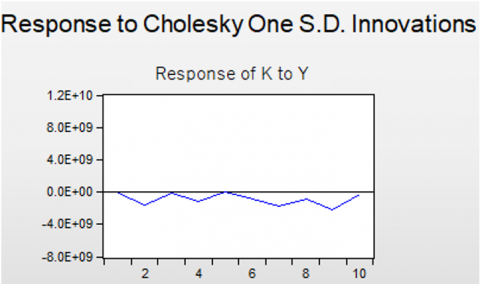
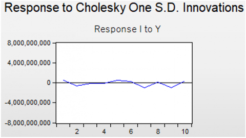
Figure 4 shows the investment response as a result of an economic growth shock. The shock from economic growth was responded to by investment which initially tended to decline in the 2nd period and towards the balance line in the 3rd to 4th period. Meanwhile, the 6th period tended to decline until the 7th period before reaching a balance point in the 8th period. This shows that the investment response resulting from a shock to economic growth is not permanent because the investment response line moves toward the balance line.
Figure 3. IRF results of consumption response due to economic growth shock
Figure 4. IRF results of investment response due to economic growth shock
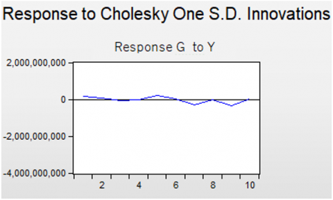
Figure 5. IRF results of government expenditure response due to shock economic growth
Figure 5 shows the response to government spending as a result of an economic growth shock. The shock from economic growth was responded to by government spending, which initially tended to decrease in the 4th period and responded with an increase in the 5th period, before decreasing in the 6th period. Meanwhile, the 8th period reached a balance point. These results indicate that the response to government spending resulting from a shock to economic growth is not permanent because the response line moves towards the balance line.
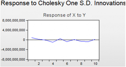
Figure 6 shows the export response as a result of an economic growth shock. The shock from economic growth was responded to by export initially tending to decline in the 4th period, and responded with an increase in the 5th period, before declining in the 6th period. In addition, the 7th period reached a balance point, and the 8th period again declined before finally reaching the balance point in the 10th period. These results indicate that the export response as a result of an economic growth shock is not permanent because the response line moves toward the balance line.
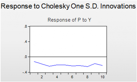
Figure 7 shows the response to the poverty rate as a result of an economic growth shock. The shock from economic growth was responded to by the poverty rate, which initially decreased not too deep in period 2 and tended to level off in periods 4, 6, and 8. These results indicate that the poverty rate response was not moving towards a balance point and was getting further away. The shock from economic growth is permanent because the response line moves away from the balance line.
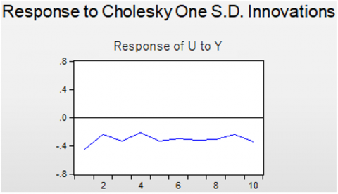
Figure 8 shows the response to the unemployment rate as a result of an economic growth shock. The shock from economic growth was responded to by the unemployment rate initially dropping deep in period 1, and tending to increase in period 2. In periods 6 and 8 it moved with a flat response before reaching a decline in period 10. These results show that the unemployment rate response is not toward the balance point and is getting further away. The shock from economic growth is permanent because the response line moves away from the balance line.
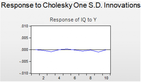
Figure 9 shows the income inequality response as a result of an economic growth shock. The shock from economic growth was responded to by income inequality, initially at a balance point in period 2, then decreased in period 3. After that, periods 4 and 5 reached a balance point, although they moved slightly towards an increase, likewise in periods 8 and 10 reached a balance point. These results indicate that the income inequality response is not permanent because the response line moves toward the equilibrium line.
Figure 6. IRF results of export response due to economic growth shock
Figure 7. IRF results of poverty-level response due to shock economic growth
Figure 8. IRF results of unemployment rate due to shock economic growth
Figure 9. IRF results of income inequality response due to economic growth shock
4.7 Forecast error variance decomposition (FEVD)
Forecast error variance decomposition (FEVD) is an analysis that provides information regarding the dynamic relationship between endogenous and endogenous variables in a dynamic VAR system. FEVD is a shock from the factors that affect certain variables' variability (fluctuation) to other variables, which are carried out orthogonally. FEVD is carried out to see what percentage of the role each shock plays in the variability of certain variables or examines the sources of fluctuations in certain variables. Thus, it can be known with certainty the factors that influence the fluctuation of a variable on other variables. Moreover, these factors are policy implications that play an important role in the stability of these variables.
Table 6 shows the results of the FEVD model of Indonesia's macroeconomic variable shock response analysis. The table shows that the variability of consumption in the short term can be explained by the shock of economic growth of 0.00% and in the long term of 11.60%. Investment variability in the short term is explained by the economic growth shock of 0.00%; in the long term, it decreases to 1.85%. The variability of government spending in the short term can be explained by the shock of economic growth of 0.00% and in the long term of 0.96%. Export variability in the short term is explained by the economic growth shock of 0.00%; in the long term, it decreases to 9.28%. The variability of the poverty rate in the short term can be explained by the shock of economic growth of 0.00% and in the long term of 2.79%. The variability of the unemployment rate in the short term is explained by the economic growth shock of 0.00%, and in the long term, it decreases to 7.64%. Finally, the variability of income inequality in the short term is explained by the economic growth shock of 0.00%, and in the long term, it decreases to 0.32%.
From the results of the FEVD, it can be concluded that economic growth has the greatest long-term impact on consumption, export, and the unemployment rate. These results prove that in the long run, economic growth can positively impact increasing consumption, export and reducing the unemployment rate. In addition, the short-term impact will be minimal, such as investment, government spending, the poverty rate, and income inequality. These results prove that economic growth can still not impact these variables significantly, so it takes time in the long term to have a more optimal impact.
Table 6. FEVD results of variable shock response analysis Indonesian macroeconomics
|
Variance Decomposition of PE: |
|||||||||
|
Period |
S.E. |
Y |
K |
I |
G |
X |
P |
U |
IQ |
|
1 |
4.378235 |
100.0000 |
0.000000 |
0.000000 |
0.000000 |
0.000000 |
0.000000 |
0.000000 |
0.000000 |
|
2 |
4.956648 |
88.53971 |
7.738778 |
0.327838 |
0.001958 |
0.022297 |
0.924494 |
1.757171 |
0.687749 |
|
3 |
5.477767 |
76.85029 |
14.08079 |
0.463487 |
0.946401 |
1.955197 |
2.809184 |
2.330250 |
0.564401 |
|
4 |
6.012726 |
74.41335 |
13.60792 |
1.198160 |
0.799188 |
1.655634 |
3.199482 |
4.631522 |
0.494741 |
|
5 |
6.533003 |
74.04293 |
11.61285 |
1.332666 |
0.777601 |
3.709387 |
3.021030 |
5.077525 |
0.426011 |
|
6 |
6.827491 |
73.13890 |
11.25438 |
1.744681 |
0.824366 |
3.425781 |
3.261646 |
5.948903 |
0.401345 |
|
7 |
7.293664 |
70.28646 |
9.863935 |
1.870372 |
0.860389 |
6.598993 |
3.436349 |
6.703633 |
0.379868 |
|
8 |
7.750947 |
69.31212 |
10.79521 |
1.688179 |
0.833447 |
6.814422 |
3.170377 |
7.049688 |
0.336561 |
|
9 |
8.097860 |
67.87282 |
10.17339 |
1.550615 |
0.929231 |
8.024421 |
3.100746 |
7.979450 |
0.369327 |
|
10 |
8.629491 |
65.52596 |
11.60178 |
1.853937 |
0.968682 |
9.285008 |
2.790878 |
7.648217 |
0.325545 |
Based on the results of the research and discussion, it can be concluded that there are several variables that have a causal relationship. Firstly, there is a causal relationship between unemployment and export, as well as between unemployment and poverty. Secondly, there is also a causal relationship between poverty and export. Thirdly, there is a bidirectional causal relationship between unemployment and poverty. Furthermore, several variables have a one-way relationship, including economic growth affecting consumption, consumption affecting government spending, government spending affecting investment, and investment affecting export.
This study provides several policy recommendations, including policies to address unemployment, in which the government needs to improve the quality and quality of the productive age workforce through guidance and counseling on work skills at vocational training centers. Furthermore, if the quality of the workforce has increased, the government also needs to increase the quantity of the employment sector through revenue from fiscal policies for various developments, which will create new job opportunities thereby reducing the unemployment rate.
Furthermore, policies to encourage export include the government being able to provide several conveniences for producers of export goods. Policies that support increasing export include ease of obtaining permits and providing facilities to producers of export goods. Facilities can be in the form of providing technology assistance, product innovation training, low interest credit assistance. This will make producers become enthusiastic about production. Relatively cheap prices for factors of production can reduce selling prices, thus increasing the competitiveness of companies.
Then, policies for poverty alleviation include improving the access of the poor to basic services. Access to education, health, clean water and sanitation, as well as food and nutrition services will help reduce costs for the poor. On the other hand, increased access to basic services encourages increased investment in human capital.
In addition, policies to increase consumption include facilitating households with stable incomes to desire consumption. This step can be carried out, for example, with the support of 0 percent installments for shopping, shopping coupons for poor and vulnerable household classes, health protocol infrastructure facilities in shopping centers, and regular festivals related to shopping.
On the other hand, policies to increase government spending include taxes, which are used to finance the budget related to development and state interests. As a source of state revenue, taxes function to finance state expenditures. Taxes are used to carry out routine state tasks and carry out development.
Finally, policies to encourage investment include establishing the Indonesia Investment Authority (INA). The establishment of INA aims to gain investors' trust by having an investment institution with good governance. In addition, to increase, prioritize and optimize long-term investments to support sustainable development. In addition, INA is also expected to improve the investment climate in Indonesia.
The limitations of this study are in the research methodology because all the variables in this study are endogenous and only analyze balance for the long term. Future research should apply the simultaneous equation approach to consider exogenous variables and can also apply an error correction model (ECM) approach that does not only analyze long-term balances but also for the short term.
The authors would like to thank Lembaga Penelitian dan Pengabdian Masyarakat Universitas Negeri Padang for funding this work with a contract number: 785/UN35.13/LT/2022.
[1] Sahnoun, M., Abdennadher, C. (2019). Causality between inflation, economic growth and unemployment in North African countries. Economic Alternatives, 29(1): 77-92.
[2] Folawewo, A.O., Adeboje, O.M. (2017). Macroeconomic determinants of unemployment: Empirical evidence from economic community of West African states. African Development Review, 29(2): 197-210. https://doi.org/10.1111/1467-8268.12250
[3] Aimon, H., Putri, K.A., Ulfa, S.S. (2022). Employment opportunities and income analysis before and during COVID-19: Indirect least square approach. Studies in Business and Economics, 17(2): 5-22. https://doi.org/10.2478/sbe-2022-0022
[4] Adeleye, B.N., Gershon, O., Ogundipe, A., Owolabi, O., Ogunrinola, I., Adediran, O. (2020). Comparative investigation of the growth-poverty-inequality trilemma in Sub-Saharan Africa and Latin American and Caribbean Countries. Heliyon, 6(12): e05631. https://doi.org/10.1016/j.heliyon.2020.e05631
[5] Benfica, R., Cunguara, B., Thurlow, J. (2019). Linking agricultural investments to growth and poverty: An economywide approach applied to Mozambique. Agricultural Systems, 172: 91-100. https://doi.org/10.1016/j.agsy.2018.01.029
[6] Statistik, B.P. (2009). Statistik Indonesia 2009 [Statistical Yearbook of Indonesia 2009]. Jakarta: BPS.
[7] Kurniadi, A.P. (2021). Determinants of biofuels production and consumption, green economic growth and environmental degradation in 6 Asia Pacific countries: A simultaneous panel model approach. International Journal of Energy Economics and Policy, 11(5): 460-471. http://dx.doi.org/10.32479/ijeep.11563
[8] Ouyang, Y., Li, P. (2018). On the nexus of financial development, economic growth, and energy consumption in China: New perspective from a GMM panel VAR approach. Energy Economics, 71: 238-252. https://doi.org/10.1016/j.eneco.2018.02.015
[9] İşleyen, Ş., Altun, Y., Görür, Ç. (2017). The causality relationship between interest rate and income with investment in USA: 1965-2016. The Journal of Academic Social Science, 5(60): 146-163.
[10] Obinna, O. (2020). Impact of interest rate deregulation on investment growth in Nigeria. International Journal of Economics and Financial Issues, 10(2): 170-180.
[11] Hicham, A. (2020). Money supply, inflation, and economic growth: Co-integration and causality analysis. Studia Universitatis Babes Bolyai-Oeconomica, 65(2): 29-45. http://dx.doi.org/10.2478/subboec-2020-0008
[12] Aimon, H., Kurniadi, A.P., Triani, M. (2022). Determination of natural gas consumption and carbon emission in natural gas supplying countries in asia pacific. International Journal of Energy Economics and Policy, 12(6): 96. https://doi.org/10.32479/ijeep.13536
[13] Afzal, M., Malik, M.E., Begum, I., Sarwar, K., Fatima, H. (2012). Relationship among education, poverty, and economic growth in pakistan: an econometric analysis. Journal of Elementary Education, 22(1): 23-45.
[14] Aimon, H., Kurniadi, A.P., Amar, S. (2021). Analysis of fuel oil consumption, green economic growth and environmental degradation in 6 Asia Pacific countries. International Journal of Sustainable Development and Planning, 16(5): 925-933. http://dx.doi.org/10.18280/ijsdp.160513
[15] Agénor, P.R., Lim, K.Y. (2018). Unemployment, growth and welfare effects of labor market reforms. Journal of Macroeconomics, 58: 19-38. https://doi.org/10.1016/j.jmacro.2018.08.009
[16] Dinh, D.V. (2020). Impulse response of inflation to economic growth dynamics: VAR model analysis. The Journal of Asian Finance, Economics, and Business, 7(9): 219-228. https://doi.org/10.13106/jafeb.2020.vol7.no9.219
[17] Bala, U., Ibrahim, A., Hadith, N.B. (2020). Impact of population growth, poverty and unemployment on economic growth. Asian Business Research Journal, 5: 48-54. https://doi.org/10.20448/journal.518.2020.5.48.54
[18] Wan, G., Hu, X., Liu, W. (2021). China's poverty reduction miracle and relative poverty: Focusing on the roles of growth and inequality. China Economic Review, 68: 101643. https://doi.org/10.1016/j.chieco.2021.101643
[19] Nwosa, P.I. (2014). Government expenditure, unemployment and poverty rates in Nigeria. Journal of Research in National Development, 12(1): 77-84.
[20] Asif, K. (2013). Factors effecting unemployment: A cross country analysis. International Journal of Academic Research in Business and Social Sciences, 3(1): 219-230.
[21] Ratnawati, K. (2020). The impact of financial inclusion on economic growth, poverty, income inequality, and financial stability in Asia. The Journal of Asian Finance, Economics, and Business, 7(10): 73-85. https://doi.org/10.13106/jafeb.2020.vol7.no10.073
[22] Dornbusch, R., S.F. (2015). Macroeconomics. India: McGraw-Hill Education.
[23] Chu, A.C.H. (2020). Advanced Macroeconomics: An Introduction for Undergraduates. World Scientific.
[24] Romer, D. (2018). Macroeconomic Theory. University of California, Berkeley.
[25] https://www.bps.go.id/, accessed on Dec. 28, 2022.
[26] Husin, H. (2022). The effect of household consumption, government spending and international trade on economic growth. Jurnal Cafetaria, 3(2): 101-110.
[27] Güngör, H., Ringim, S.H. (2017). Linkage between foreign direct investment, domestic investment, and economic growth: evidence from Nigeria. International Journal of Economics and Financial Issues, 7(3): 97-104.
[28] Satrianto, A., Juniardi, E. (2023). Inclusive human development and inclusive green growth: A simultaneous approach. International Journal of Sustainable Development and Planning, 18(2): 523-530. https://doi.org/10.18280/ijsdp.180221
[29] Bakari, S., Mabrouki, M. (2017). Impact of exports and imports on economic growth: new evidence from Panama. Journal of Smart Economic Growth, 2(1): 67-79. https://jseg.ro/index.php/jseg/article/view/70/60.
[30] Amar, S., Satrianto, A., Ariusni, Kurniadi, A.P. (2022). Determination of poverty, unemployment, economic growth, and investment in West Sumatra province. International Journal of Sustainable Development and Planning, 17(4): 1237-1246. https://doi.org/10.18280/ijsdp.170422
[31] Soylu, Ö.B., Çakmak, İ., Okur, F. (2018). Economic growth and unemployment issue: Panel data analysis in Eastern European Countries. Journal of International Studies, 11(1): 93-107. http://dx.doi.org/10.14254/2071-8330.2017/11-1
[32] Yang, Y., Greaney, T.M. (2017). Economic growth and income inequality in the Asia- Pacific region: A comparative study of China, Japan, South Korea, and the United States. Journal of Asian Economics, 48: 6-22. https://doi.org/10.1016/j.asieco.2016.10.008
[33] Karim, Z.A., Karim, B. A., Ahmad, R. (2010). Fixed investment, household consumption, and economic growth: A structural vector error correction model (SVECM) study of Malaysia. https://mpra.ub.uni-muenchen.de/id/eprint/27146.
[34] Herrendorf, B., Rogerson, R., Valentinyi, A. (2021). Structural change in investment and consumption—A unified analysis. The Review of Economic Studies, 88(3): 1311-1346. https://doi.org/10.1093/restud/rdaa013
[35] Baker, S.R., Yannelis, C. (2017). Income changes and consumption: Evidence from the 2013 federal government shutdown. Review of Economic Dynamics, 23: 99-124. https://doi.org/10.1016/j.red.2016.09.005
[36] Tampubolon, J., Loh, A. (2020). The effects of domestic demand and export on economic growth of North Sumatra. Jurnal Ekonomi dan Studi Pembangunan, 12(2): 108- 126. http://dx.doi.org/10.17977/um002v12i22020p108
[37] Nelson, T., McCracken-Hewson, E., Sundstrom, G., Hawthorne, M. (2019). The drivers of energy-related financial hardship in Australia–understanding the role of income, consumption and housing. Energy Policy, 124: 262-271. https://doi.org/10.1016/j.enpol.2018.10.003
[38] Anghel, B., Basso, H., Bover, O., Casado, J.M., Hospido, L., Izquierdo, M., Kataryniuk, I.A., Lacuesta, A., Montero, J.M., Vozmediano, E. (2018). Income, consumption and wealth inequality in Spain. SERIEs, 9: 351-387. https://doi.org/10.1007/s13209-018-0185-1
[39] Kaplanoglou, G., Rapanos, V.T. (2018). Evolutions in consumption inequality and poverty in Greece: The impact of the crisis and austerity policies. Review of Income and Wealth, 64(1): 105-126. https://doi.org/10.1111/roiw.12287
[40] Sims, E., Wolff, J. (2018). The output and welfare effects of government spending shocks over the business cycle. International Economic Review, 59(3): 1403-1435. https://doi.org/10.1111/iere.12308
[41] Blanchard, E.J., Olney, W.W. (2017). Globalization and human capital investment: Export composition drives educational attainment. Journal of International Economics, 106: 165-183. https://doi.org/10.1016/j.jinteco.2017.03.004
[42] Aimon, H., Putri, K.A., Ulfa, S.S. (2022). Employment opportunities and income analysis before and during COVID-19: indirect least square approach. Studies in Business and Economics, 17(2): 5-22. https://doi.org/10.2478/sbe-2022-0022
[43] Steinert, J.I., Zenker, J., Filipiak, U., Movsisyan, A., Cluver, L.D., Shenderovich, Y. (2018). Do saving promotion interventions increase household savings, consumption, and investments in Sub-Saharan Africa? A systematic review and meta-analysis. World Development, 104: 238-256. https://doi.org/10.1016/j.worlddev.2017.11.018
[44] Ganchev, G., Todorov, I. (2021). Taxation, government spending, and economic growth: The case of Bulgaria. Journal of Tax Reform, 7(3), 255-266. https://doi.org/10.15826/jtr.2021.7.3.102
[45] Vasilev, A. (2018). Optimal fiscal policy with utility-enhancing government spending, consumption taxation and a common income tax rate: The case of Bulgaria. Review of Economics, 69(1): 43-58. https://doi.org/10.1515/roe-2017-0022
[46] Boehm, C.E. (2020). Government consumption and investment: Does the composition of purchases affect the multiplier?. Journal of Monetary Economics, 115: 80-93. https://doi.org/10.1016/j.jmoneco.2019.05.003
[47] Antonelli, M.A., De Bonis, V. (2019). The efficiency of social public expenditure in European countries: A two-stage analysis. Applied Economics, 51(1): 47-60. https://doi.org/10.1080/00036846.2018.1489522
[48] Sunde, T. (2017). Foreign direct investment, exports, and economic growth: ADRL and causality analysis for South Africa. Research in International Business and Finance, 41: 434-444. https://doi.org/10.1016/j.ribaf.2017.04.035
[49] Wang, H., Yang, M., He, R., Zheng, P. (2022). Environmental regulation, foreign direct investment, and export sophistication of China: an empirical study based on dynamic system GMM and threshold model. Environmental Science and Pollution Research, 29(48): 72090-72100. https://doi.org/10.1007/s11356-021-14833-2
[50] Hok, L., Bartha, Z. (2022). The optimal magnitude of government spending: evidence from Cambodia. South Asian Journal of Macroeconomics and Public Finance, 22779787221093116. https://doi.org/10.1177/22779787221093116
[51] Lwesya, F. (2018). Export diversification and poverty reduction in Tanzania. Romanian Economic Journal, 20(68): 93-110.
[52] Dritsakis, N., Stamatiou, P. (2018). Causal nexus between FDI, exports, unemployment, and economic growth for the old European union members. evidence from panel data. International Journal of Economic Sciences, 7(2): 35-56. http://dx.doi.org/10.20472/ES.2018.7.2.002
[53] Cruz, M., Ahmed, S.A. (2018). On the impact of demographic change on economic growth and poverty. World Development, 105: 95-106. https://doi.org/10.1016/j.worlddev.2017.12.018
[54] Martin, A., Markhvida, M., Hallegatte, S., Walsh, B. (2020). Socio-economic impacts of COVID-19 on household consumption and poverty. Economics of Disasters and Climate Change, 4(3): 453-479. https://doi.org/10.1007/s41885-020-00070-3
[55] Lenz, L., Munyehirwe, A., Peters, J., Sievert, M. (2017). Does large-scale infrastructure investment alleviate poverty? Impacts of Rwanda’s electricity access roll-out program. World Development, 89: 88-110. https://doi.org/10.1016/j.worlddev.2016.08.003
[56] Rodríguez-Castelán, C., Vazquez, E., Winkler, H. (2020). Tracing the local impacts of exports on poverty and inequality in Mexico. IZA Discussion Paper, No. 13610. http://dx.doi.org/10.2139/ssrn.3679016
[57] Evans, O., Kelikume, I. (2019). The impact of poverty, unemployment, inequality, corruption, and poor governance on Niger Delta militancy, Boko Haram terrorism, and Fulani herdsmen attacks in Nigeria. International Journal of Management, Economics and Social Sciences (IJMESS), 8(2): 58-80. https://doi.org/10.32327/IJMESS/8.2.2019.5
[58] Leasiwal, T.C. (2021). A longitudinal analysis of the effect of wages, inflation, economic growth on unemployment rate in Maluku Province, Indonesia. International Journal of Entrepreneurship, 25: 1-11.
[59] Alper, A. (2018). The relationship of economic growth with consumption, investment, unemployment rates, saving rates, and portfolio investments in the developing countries. Gaziantep University Journal of Social Sciences, 17(3): 980-987. https://doi.org/10.21547/jss.342917
[60] Omran, E.A.M., Bilan, Y. (2020). The impact of fiscal policy on the unemployment rate in Egypt. Montenegrin Journal of Economics, 16(4): 199-209. https://doi.org/10.14254/1800-5845/2020.16-4.16
[61] Mohammad, U.F., David, J. (2019). The relationship between poverty and unemployment in Niger state. Signifikan, 8(1): 71-78. https://doi.org/10.15408/sjie.v8i1.6725
[62] Amri, K. (2018). Is there causality relationship between economic growth and income inequality?: Panel data evidence from Indonesia. Eurasian Journal of Economics and Finance, 6(2): 8-20.