

Abstract
The first application of time-dependent probability density function (PDF) analysis to the L-H transition in fusion plasmas is presented. PDFs are constructed using Doppler Backscattering data of perpendicular fluctuation velocity,  , and turbulence from the edge region of the DIII-D tokamak. These raw time-series data are sliced into millisecond-long sliding time-windows to create PDFs. During the transition, the
  PDFs develop strong right tails, indicative of turbulence-suppressing localised flows in the plasma edge; such features and other subtle behaviours are explored using novel information geometry techniques. This letter examines the applicability of these techniques to predict L-H transitions and investigate predator-prey self-regulation theories between turbulence and perpendicular velocity.
Export citation and abstract BibTeX RIS

Published by the EPLA under the terms of the Creative Commons Attribution 4.0 International License (CC-BY). Further distribution of this work must maintain attribution to the author(s) and the published article's title, journal citation, and DOI.
Introduction
Nuclear fusion has been studied as a potential energy source since the 1940s [1], but scientific and engineering progress has accelerated in the last few decades as the clear need for sustainable power has grown [2]. Crucial to achieving sustained magnetically confined fusion is the controlled access to a steady state high-confinement regime of operation known as H-mode [3,4]. This, in turn, requires an in-depth understanding and physics-based model of the low-confinement to high-confinement (L-H) and reverse high-confinement to low-confinement (H-L) transitions [5–7].
The current paradigm for sustained H-mode has been experimentally verified to be due to the suppression of edge plasma turbulence by sheared zonal and mean flows, leading to enhanced confinement [8,9]. The question of the trigger mechanism or spatio-temporal causality of the sheared flow, and correlation with turbulence flow energy transfer, remains an area of ongoing research; it has been suggested [6,10], and demonstrated experimentally [11], that turbulence itself is capable of driving these zonal flows in the first place.
In addition, it is not understood why some transitions rapidly reach H-mode through a sharp bifurcation of state and corresponding reduction in turbulence, while other transitions dither between H- and L-mode-like phases through so-called limit-cycle oscillations (LCO) [9,12,13] before the H-mode is reached.
Since H-mode transitions (L-H, H-L, L-LCO) are abrupt events that cause sudden changes in the plasma transport, the system is characterised by time-variability and large fluctuations in the causal variables. Conventional analysis approaches, which use assumed Gaussian distributions and associated mean and standard deviation values, result in the loss of valuable information over the very short L-H/H-L transition timescales. An alternative approach to studying very fast phenomena is the use of non-stationary, statistical methods such as time-dependent probability density functions (PDFs).
By analysing the PDFs of the measured experimental parameters thought to contribute to the H-mode transitions, information geometry can be used to quantify how the information and statistical states unfold over time [14]. This also enables key variables with different physical units to be compared in terms of dimensionless numbers (changes in statistical states), measuring to what degree they might be correlated. Furthermore, subtle changes in PDFs can be detected on time-scales relevant to the L-H and L-dithering-H transitions, allowing the dynamics of key linked variables to be explored.
The main aim of this letter is to report the first calculation of time-dependent PDFs from time-series edge plasma experimental data across H-mode transitions and the application of information geometry analysis. Our novel analysis technique is applied to a sharp and a dithering transition separately to improve our understanding of the evolution of edge plasma turbulence and flow velocities in the L-H transition under different experimental scenarios. This new method is shown to provide tools for capturing the complex evolution of the L-H transition, with promising potential for predicting the onset of the transitions.
Density fluctuation and velocity measurements
The DIII-D Doppler Backscattering (DBS) diagnostic [15] is used to provide high temporal and spatial resolution measurements of the plasma turbulence in terms of relative electron density fluctuation,  , and perpendicular fluctuation velocity,
  [16]. This velocity is calculated from the backscattered signal, which has a doppler shift
  , where
  is the perpendicular wave number of the turbulence;
  ranges from
  to
to  . The fluctuation velocity,
  , is the sum of the plasma mean
  velocity,
  , and the turbulence phase velocity, vph
, meaning that the
, and the turbulence phase velocity, vph
, meaning that the  measurements are sensitive to changes in
  and zonal flows. The study presented in this letter focuses on these two measured variables,
  and
and  , which are understood to have important roles in the triggering and evolution of the L-H and H-L transitions.
Constructing time-dependent PDFs from time traces of experimental data requires good statistical samples, and thus data with high sampling frequency. This was achieved by using sliding time-windows of fixed duration to sample the DBS data and make a histogram, resulting in good-quality time-dependent PDFs. A full analysis of the uncertainties has been carried out and errors are provided for the PDF animations in the Supplementary Material Supplementarymaterial.pptx (SM).
The DBS diagnostic uses eight channels at different frequencies to probe the eight radial edge plasma locations shown in fig. 1 as a function of ρ, the normalized radius between the centre of the plasma and the last closed flux surface. In this study, results are presented for the single outermost channel (channel 1). The radial probing location of channel 1 remains within the narrow (few cm) confined plasma close to the separatrix and inside the pedestal electric field gradient layer where the LCO and L-H transition dynamics occur. The same analysis was performed on channel 2, which gives an independent measurement at a slightly lower radius, and provided very similar results for the PDF analysis.
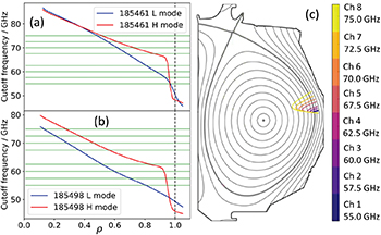
Fig. 1: X-mode cut-off frequencies in L-mode (blue) and H-mode (red) for shots (a) 185461 and (b) 185498 along with channel frequencies (green) plotted as a function of ρ. (c) DIII-D poloidal cross-section with the eight channel beam trajectories obtained by ray tracing. The innermost point reached for each beam is taken as the probed radius.
Download figure:
Standard imageThe DBS diagnostic has a temporal resolution of  and a typical spatial resolution ranging from 0.5 to 2 cm. The level of turbulence is proportional to the signal intensity. Values of
  have been determined from a 128-point Fourier transformation of the raw signal to evaluate the Doppler shift, meaning that the time resolution and available number of
  data points in a given time-window is 128 times smaller than for the
  measurements.
Statistical analysis
Sharp L-H and H-L transitions occur in under 1 ms, while dithering LCOs can have time periods of 0.3–10 ms; therefore, short time-windows of a few ms are essential for analysing and observing H-mode transition dynamics. However, generating PDFs from data using very short time-windows reduces the number of data points sampled, which can degrade the quality of the PDFs and the amount of information derived from them. The choice of time-window for the PDFs will depend on the temporal resolution of the diagnostic and the types of transitions being analysed; for this analysis a minimum of 50 data points per time-window was required for meaningful interpretation of the PDFs. For these data, time-windows of  for turbulence and
  for
for  were found to be optimal.
The time-dependent PDFs, p(x, t), of a stochastic variable x can be analysed by the time evolution of their moments, such as standard deviation, σ, and kurtosis, K. However, these low-order moments have limitations in understanding non-Gaussian statistical properties, particularly under non-equilibrium conditions involving large fluctuations. In this letter, a non-perturbative method is used to capture the evolution of the entire PDFs, from the perspective of geometry, by quantifying their temporal change in terms of a dimensionless distance (metric). This enables the interpretation of the evolution of different variables  in terms of the same dimensionless numbers and provides a novel and promising methodology to study and compare different stochastic processes, such as phase transitions (for example, see [14,17]) with the variables, information length and rate.
Specifically, based on the relative change between two temporally adjacent PDFs, the square of information rate,  , and information length,
  [14,17], are calculated as follows:


where  . To avoid numerical problems when calculating
  for very small values of p(x, t) in eq. (1), the second expression is used in these calculations.
Note that  in eq. (2) gives a dimensionless measure of the total number of statistically different states that p(x, t) evolves through in the time interval (0, t). Information length,
  , can be envisioned as a measure of the statistical distance between two time-dependent PDFs, which represents the system's trajectory in probability space [14,18,19], whereas
  measures the instantaneous change in statistical states. For a Gaussian PDF, a statistically different state can be defined as a change in the mean value, or due to a change in width, σ. Information length,
  , is proportional to the time integral of the square root of the information rate,
  , defined in eq. (1). To understand the L-H transition with and without dithering,
  and
and  are calculated from the time-dependent PDF
  , and similarly
  and
and  are calculated from the PDF
  .
.
Since information geometry tools were developed for continuous PDFs, care must be taken when applying these equations to discrete data. To minimize artificial spikes caused by the discrete derivative in eq. (1),  is computed between PDFs 1 ms apart. These small increments of
  provide sufficient precision in the values of
  and
and  to observe important L-H transition effects, whilst avoiding large discontinuities from discrete data.
L-H transition data
The general parameters for the shots used in this study, one sharp transition and one dithering transition, are shown in fig. 2. These plasmas were part of a dedicated L-H transition investigation on DIII-D at plasma current,  and toroidal magnetic field,
  . Both transitions took place in the initial NBI-only auxiliary heating phase, with shot 185461 operating with the small angle slot (SAS) divertor configuration [20], and 185498 with the conventional "partially open" divertor configuration.
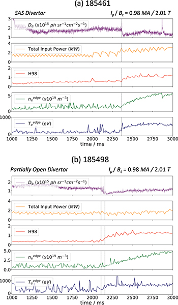
Fig. 2: General parameters and variables for (a) shot 185461 (sharp transition) and (b) shot 185498 (dithering transition), showing  intensity, total input power, H98, edge ne
and edge Te
. The dashed line in (a) marks the L-H transition, and the dashed lines in (b) mark the start and end of the dithering phase.
intensity, total input power, H98, edge ne
and edge Te
. The dashed line in (a) marks the L-H transition, and the dashed lines in (b) mark the start and end of the dithering phase.
Download figure:
Standard imageThe L-H transition for shot 185461 occurred at  at a line-averaged electron density
  and a power threshold
  . The power threshold is defined by the equation
  , where PNBI
is the NBI heating power, POH
is the Ohmic power and
, where PNBI
is the NBI heating power, POH
is the Ohmic power and  is the rate of change of the stored plasma energy. The plasma transitioned directly to an ELM-free H-mode phase with an accompanying sharp drop in the divertor
  emission and a rise in the edge electron density, ne
edge
, and plasma confinement, H98, shown by the time traces in fig. 2(a).
emission and a rise in the edge electron density, ne
edge
, and plasma confinement, H98, shown by the time traces in fig. 2(a).
The second plasma, 185498, transitioned to a dithering H-mode or LCO phase at  , with
  and
and  . The dithering phase oscillations lasted for 50 ms before the shot entered an ELM-free H-mode, shown along with the other plasma parameters in fig. 2(b).
The radial profiles of ne
, electric field, Er
, and  in fig. 3 at times before and after the L-H transitions, show the formation of the ne
pedestal and Er
well for both plasmas, as well as the clear correlation between
in fig. 3 at times before and after the L-H transitions, show the formation of the ne
pedestal and Er
well for both plasmas, as well as the clear correlation between  and Er
. For shot 185461, channel 1's probed radius (pink shading) remained in the steep pedestal gradient and Er
well region (ρ = 0.97–0.98). In shot 185498, channel 1 covered a wider range (ρ = 0.85–0.95), corresponding to the top and steep gradient regions of the pedestal, and the inner part of the Er
well.
and Er
. For shot 185461, channel 1's probed radius (pink shading) remained in the steep pedestal gradient and Er
well region (ρ = 0.97–0.98). In shot 185498, channel 1 covered a wider range (ρ = 0.85–0.95), corresponding to the top and steep gradient regions of the pedestal, and the inner part of the Er
well.
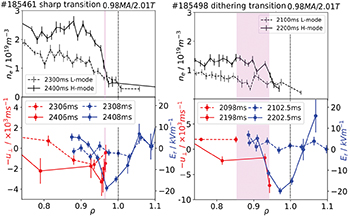
Fig. 3: Edge radial profiles for shot 185461 and 185498 showing ne
from Thomson Scattering (black),  from DBS (red) and radial electric field from Charge Exchange Recombination Spectroscopy (blue). The L- and H-modes are represented by the dashed and solid lines respectively. The pink shaded regions show the radial range probed by the DBS channel 1.
Download figure:
Standard imageExamples of the PDFs  and
and  around the L-H transitions are shown in fig. 4(a) and fig. 5(a) for
  and fig. 4(b) and fig. 5(b) for
  , along with animations of the time-dependent PDF evolution at every millisecond in the SM. The number of bins used to construct the PDFs for the two measurements was determined using the Rice rule [21], resulting in 11 and 34 bins for
  and
and  , respectively. A kernel density estimation method [22] for smoothing the PDFs was tested and found only to slow down the calculations without meaningfully altering the results; therefore, no filtering was applied. When comparing,
  appears smoother than
  because
  contains 128 times more data points.
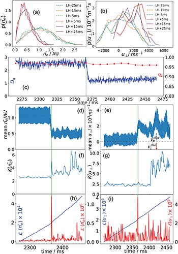
Fig. 4: Statistical properties of shot 185461, which undergoes a sharp L-H transition at  : (a) time-dependent PDFs of
  (arbitrary units AU) and (b)
  for different times before and after the L-H transition. (c) The
  intensity (blue) and ρ (red) probed by the DBS diagnostic as a function of time. Mean values and standard deviations, σ (denoted by error bars), for (d)
  and (e)
  against time. Vertical arrows show the direction of electron (blue) and ion (red) diamagnetic drift velocities,
  and
and  . Kurtosis, K, for (f)
  and (g)
  against time. Information length,
  (blue), and information rate,
  (red), for (h)
  and (i)
  against time. In (c)–(f), the L-H transition is marked by the green vertical line.
Download figure:
Standard image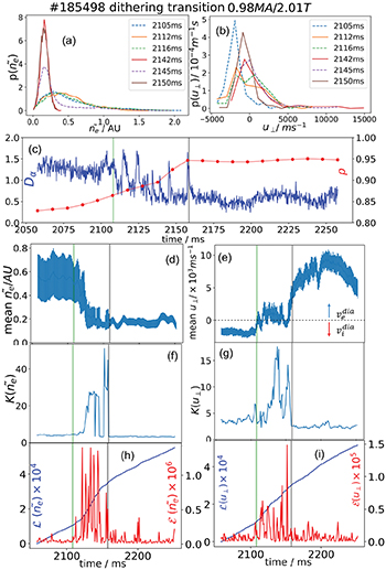
Fig. 5: The same as fig. 4, but for a shot 185498 undergoing a dithering L-H transition at  ; in (c)–(f) the green and grey vertical lines mark the L mode-to-dithering and dithering-to-H mode transitions, respectively.
Download figure:
Standard imageThe experimental parameters, such as the divertor magnetic configuration, L-mode  and Pth
, are different for these two shots. A direct comparison of the stochastic model analysis of the transition dynamics would therefore provide limited insight and is not made here.
and Pth
, are different for these two shots. A direct comparison of the stochastic model analysis of the transition dynamics would therefore provide limited insight and is not made here.
In the following sections, results are presented from the statistical analysis applied to two separate shots with distinct L-H transitions, sharp and dithering. These two shots provide a robust representation of the results from a comprehensive application of the time-dependent PDF analysis to all eight DBS channel data for all plasmas in the L-H transition investigation.
Sharp L-H transition
PDF analysis
For shot 185461 with a sudden transition to an ELM-free H-mode at  (fig. 4(a)),
  shows a sharp change from a relatively wide distribution in the L-mode phase (dotted lines) with standard deviation
  (green PDF), to a narrow and asymmetric distribution in the H-mode (solid lines) with
  (red PDF).
While detailed analysis of the changes in PDF structure for this rapid transition is challenging, important behaviour is observed. Specifically, going from the orange to the green PDF curve involves the shortening of the right tail in  , beyond the PDF uncertainties, with hardly any accompanying change in the left tail. This suggests only high-amplitude turbulence, with higher values of
  , is suppressed before the L-H transition. In addition, the orange and green curves appear to develop a secondary peak around
  , near the H-mode peaks, reminiscent of bimodal PDF behaviour [14,17]. In comparison, going from the green to the red curve (at the L-H transition) involves the leftward shift and narrowing of the entire
  , indicating general suppression of turbulence after the transition. Interestingly, all three
  in H-mode (red, purple, violet) exhibit a heavier right tail, extending over a wider range
  than the left tail
  , despite their narrower distribution.
When compared with  ,
,  (in fig. 4(b)) exhibits more changes across the transition. For instance,
  becomes more positive and skewed as the L-H transition is approached, and
  changes from
  to
to  around the transition. In addition, the orange and green curves appear to develop a bimodal structure. After the transition, the
  PDFs are narrower with their peaks appearing at a larger value of
  .
.
The expected decrease in the edge plasma region turbulence level at the L-H transition is clearly observed in fig. 4(d) with a sharp drop in mean  , which coincides with the sudden increase in mean
  in fig. 4(e). In H-mode, the mean values of
  and
and  vary over time, involving some quasi-oscillations with a long period
  . The physical origin of these oscillations is not entirely clear, but it is not central to the purpose of this letter and will be addressed in a future publication. It is, however, interesting to note that the local maxima of the
  oscillations tend to occur near the local minima of the
  oscillations, indicating self-regulation between the two variables.
The kurtosis,  and
and  , in fig. 4(f) and (g) is smaller than the Gaussian value of 3 in L-mode. However,
  shows a sharp peak at the transition and then a non-monotonic increase over time. Since a large kurtosis above the Gaussian value signifies heavy tails and intermittency, the
  peak at the transition indicates high-amplitude intermittency, possibly linked to the stronger suppression of high-amplitude turbulence noted above.
Interestingly, the large spikes in  around
  seem to be associated with the peaks in mean value
  in fig. 4(e), and are followed by the spikes in
  in fig. 4(g). Increased values of
  indicate the development of tails in the
  due to the growth of strong localised flows [17]. It is should be noted that for both shots, skewness was found to provide very similar results to kurtosis.
Information geometry
The temporal evolution of  and
and  in fig. 4(h) and (i) characterises the rate and accumulated temporal change of the PDFs. Sharp spikes in
  and
and  at the L-H transition reflect sudden changes in the PDF shapes at this time, thus providing clear markers for the L-H transition. A notable increase in the
  and
and  oscillations in H-mode signifies an increased number of statistical state for both variables compared with L-mode due to the quasi-oscillatory evolution of both
  and
and  in H mode. Consequently, the cumulative change in the statistical states,
  in fig. 4(h) and
  in fig. 4(i), shows shallower slopes
  in L-mode, with sudden changes in gradient at the transition;
  and
and  .
.
Dithering transition
PDF analysis
For shot 185498, the start of the dithering H-mode occurs at  and is followed by a period of LCOs. These LCOs are useful because they prolong the L-H transition dynamics, allowing the behaviour (e.g., oscillations) of key variables to be observed more clearly over a longer time period [23]. As the dithering can result from self-regulation between turbulence and zonal flows,
  is referred to as a zonal flow for the dithering transitions [10].
Statistical analysis of the dithering H-mode phase for shot 185498 is shown in fig. 5, and an expanded trace is shown in fig. 6 with detailed features of the LCOs. Overall, the L-mode  PDF (in dotted blue) in fig. 5(a) changes from a wide, even distribution to a more skewed, narrow distribution over the transition, with
  at
at  in L-mode and
  at
at  well into the dithering phase. Correspondingly,
  becomes more positive and widths grow from
  to
to  for the same times.
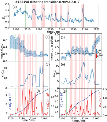
Fig. 6: An expanded view of dithering phase in fig. 5(c)–(i).
Download figure:
Standard imageSpecifically, the transition to the dithering phase (blue to orange of  ) involves the shortening of the right tail and a hint of dual peak formation around
  , which then returns to a single peak in the green curve. The shortened right tail suggests that higher-amplitude turbulence
  is suppressed by changes in the velocity prior to the transition, similar to what was observed in fig. 4 for the sharp transition. The narrowing of the
  PDF that was seen in fig. 4(a) is also observed here (from the green to the red line), indicating the perpendicular velocity suppression of both low
  and high-amplitude turbulence
  , with a PDF peaking at a much lower
  , after the transition to the dithering phase.
Further time evolution of the PDFs in solid red, dotted purple, and solid brown lines reveal the oscillation of PDF itself, as observed in [14,17]; a wider and more skewed PDF (purple) with a right tail  extended to
  , is sandwiched between two narrow, low-amplitude
  range PDFs (red and brown).
Remarkably, similar PDF oscillations are also observed for  in the red, purple and brown curves in fig. 5(b), but in such a way that the narrow PDFs of
  with a shorter right tail (red and brown) correspond to the PDFs of
  peaking around
  while the wider PDF with a heavy right tail of
  (purple) corresponds to the
  peak at
  . This is a clear demonstration of self-regulation between turbulence and zonal flows. Furthermore,
  in the H-mode–like dithering phase shows a stretched PDF right tail in comparison with the L-mode and L-mode–like phase PDFs, suggesting that strong zonal flows play a crucial role in regulating turbulence [17].
The time-trace of mean  in fig. 5(d), (e) shows no significant change until just before the transition, while the mean
  in fig. 5(e) undergoes a sudden increase in value 4 ms prior to the L-dithering phase transition (green vertical line). This increase, which is more clearly seen in the expanded trace of fig. 6(c), suggests that zonal flows trigger the initial transition from L-mode to the dithering phase. The PDF intermittency discussed above can also be seen in the time traces in fig. 5(f) and fig. 6(d);
  remains almost constant at
  over the transition to dithering, while
  in fig. 5(g) and fig. 6(e) increases sharply from 3 to 7 in the 7 ms prior to the L-dithering phase transition (green vertical line), again reflecting intermittency and the role of zonal flows in triggering the transition.
On the other hand, the mean  rises to around
  at
at  following the first transition and oscillates around that value for the remainder of the dithering phase. In comparison, the value of
  rises significantly after the first transition, peaking at 17.8 at
  , again, reflecting a strong intermittency.
Information geometry
Another important measure of zonal flows and their effect on the transition is provided by the information diagnostics in fig. 5(h), (i) and fig. 6(f), (g). Specifically, the first spike in  and the sudden change in the gradient of
  appear prior to the first phase transition indicated by the green vertical line, while the first spike in
  and the sudden change in the gradient of
  appear after the transition. This information is consistent with zonal flows triggering the dithering transition. It is quite interesting that despite the different evolution of
  and
and  during dithering, the information lengths at
  are
are  and
and  , indicating that
  and
and  undergo similar total changes in their statistical states due to their strong correlation through self-regulation. Sudden changes in gradient are observed for the L-, dithering and H-mode phases, with corresponding values of
  and
and  .
.
The seven dithering phase oscillations are more closely examined in fig. 6 to highlight the correlation between the different measured variables. The pink regions mark the time periods of high  intensity and therefore indicate the low confinement dithering phases. For four of these oscillation cycles, an increase in
  ,
,  and
and  is observed before the transition to the H-mode–like phase. The 1 ms time-windows for PDFs used to calculate
  are narrow enough to capture the detailed dynamics, but the 5 ms windows used in
  result in artificially wider peaks and some rapid changes may not be captured, although the important oscillations are still observed. For example, around half the peaks in
  appear to oscillate out of phase with peaks in
  , indicating predator-prey behaviour. In addition, the largest peak in
  occurs 6.5 ms before the final transition to the H-mode (grey), and is followed by a spike in
  1.5 ms before the transition; this suggests that the time-dependent PDF analysis of these variables has the potential to provide predictive capability for the onset of H-mode.
Conclusions
This letter presents the first application of a time-dependent PDF analysis to the sharp and dithering L-H transitions from DIII-D experimental data, using DBS measurements of edge plasma  and turbulence
  . Overall, the sharp and dithering L-H transitions exhibit complex temporal evolution involving non-Gaussian PDFs, long stretched tails and possible bi-modality, and PDF oscillations. In particular, the heavy right tails of
  suggest the presence of strong localised perpendicular (zonal) flows and their important role in turbulence regulation, as predicted theoretically [14,17]. Furthermore, evidence of two-step turbulence suppression near the transition to the H-mode and in the dithering phase has been demonstrated within the temporal resolution limits, with several cases of the localised perpendicular velocity followed by the reduction of larger amplitude turbulent structures prior to the transition, succeeded by a general suppression of turbulence. The novel information geometry diagnostics
  and
and  provide a clear marker for the sharp and dithering L-H transitions. In addition, they have potential for predictive capability, with a sharp peak in
  appearing to forecast the L-to-dithering and dithering-to-H transitions. Furthermore, the correlation between
  and
and  through self-regulation is well captured by their similar
  values, particularly in the dithering phase, providing valuable experimental evidence of the predator-prey model assumptions.
In conclusion, the time-dependent PDF analysis has been shown to be a sensitive tool for understanding the dynamic changes in the plasma across the L-H transition. This stochastic analysis approach has potential for predicting and controlling phase changes in magnetically confined plasma systems. It will be developed further, with plans for application to more L-H transition shots, higher-resolution data and other variables of interest. For example, the role of electromagnetic turbulence in H-mode transitions will be investigated along with an exploration of the cause of the H-mode quasi-oscillations observed in fig. 4.
Acknowledgments
The authors would like to acknowledge the DIII-D team, and give special thanks to Quinn Pratt and Kathreen Thome, for their assistance, support and illuminating discussions. This material is based upon work supported by the U.S. Department of Energy, Office of Science, Office of Fusion Energy Sciences, using the DIII-D National Fusion Facility, a DOE Office of Science user facility, under Award(s) DE-FC02-04ER54698, DE-SC0019352, DE-SC-0020287, and DE-FG02-08ER54999. This report was prepared as an account of work sponsored by an agency of the United States Government. Neither the United States Government nor any agency thereof, nor any of their employees, makes any warranty, express or implied, or assumes any legal liability or responsibility for the accuracy, completeness, or usefulness of any information, apparatus, product, or process disclose or represents that its use would not infringe privately owned rights. Reference herein to any specific commercial product, process, or service by trade name, trademark, manufacturer, or otherwise does not necessarily state of reflect those of the United States Government or any agency thereof.
Data availability statement: The data generated and/or analysed during the current study are not publicly available for legal/ethical reasons but are available from the corresponding author on reasonable request.