


Abstract
X-ray Compton scattering measurements have been carried out for fluid rubidium (Rb) from near the melting point up to the critical regions. The electron kinetic energy (KE) was derived from the valence Compton profiles and its relative variation as a function of the fluid density was compared with that of the electron gas model. Reduction in the KE occurs more slowly than that predicted by the model as the fluid density decreases and an apparent deviation in the KE from the model is observed at the densities where the fluid is still metallic. These findings suggest that a fluctuation intrinsic to the low-density electron gas causes charge inhomogeneity in valence electrons in real fluid rubidium, being coupled with ionic density fluctuations.
Export citation and abstract BibTeX RIS
Introduction
The fluid state of matter offers a unique opportunity where various physical properties are evaluated as a function of density, which varies greatly from the liquid phase to the vapor phase. Fluid metals are inherently characterized by the existence of conduction electrons, and significant changes in electronic behavior occur as a function of thermodynamic variables. Expansion along the coexistence curve causes a gradual loss of metallic nature, leading eventually to a metal-insulator transition [1]. The correspondence between the liquid-vapor and the metal-insulator transitions is no longer obvious in this situation, which provides a unique opportunity to investigate the nature of the metal-insulator transition in fluid metals and its relation to the liquid-vapor transition [1–4]. Among the elemental metals, alkali metals are an ideal system for such investigation because their valence electrons are well described by the electron gas model. Referring to a basic model helps to gain insight into the underlying physics of expanded fluid metals.
Electrical conductivity measurements indicated that expanded fluid Rb and Cs undergo a metal-insulator transition near the critical density  (Rb:
(Rb:  ; Cs:
; Cs:  [1]) [5]. Until the density of the fluids reaches
  , the electrical conductivity is about 103–104 (Ω cm)−1 and comparable to the nearly free electron (NFE) prediction [6,7], thus, the fluids preserve metallic characters in this density region [1]. With further density reduction, the conductivity exhibits a significant departure from the NFE behavior [6,7]. Moreover, the enhancement of the magnetic susceptibility is also observed at approximately below
  [8,9].
Since an indication was given that there is an appreciable number of diatomic molecules in fluid Cs near the liquid-vapor critical point [8], the great concern has been whether such molecular structural units persist even in the metallic liquid. Quantum-statistical calculations [10] indicated that the presence of ionized molecular species such as  or
or  can explain the enhancement in magnetic susceptibility [8,9] in the density range of about 2–3ρc. Inelastic neutron scattering measurements for fluid Rb [11,12] have revealed a vibration mode in the dynamic structure factor at approximately
  , suggesting the existence of such structural units in the fluid. X-ray diffraction measurements using synchrotron radiation for the static structure factor of fluid Rb have shown that a structural change appears in a relatively earlier stage of volume expansion (
 , 1.0–1.1 g cm−3) [13]; the nearest-neighbor distance R1 decreases in spite of volume expansion. A theoretical explanation was given that the contraction of R1 is essentially caused by the enhanced attraction between valence electrons in the low-density electron gas, combined with the exclusion effect of the electrons from the ionic cores [14]. Moreover, it was proposed that a structural modification from a dense to loose liquid already occurs in fluid Rb within a higher-density region (below 1.32 g cm−3) by the analysis based on the reverse Monte-Carlo method [15].
Toward a unified understanding of these features, direct observation of the electronic state of valence electrons is of great significance. Synchrotron-based Compton scattering has been regarded as quite an effective technique for probing the momentum density of electrons in materials [16]. Its high applicability to a wide variety of experimental conditions has also been demonstrated [17–19].
In this paper, we report the results of X-ray Compton scattering experiments for fluid Rb. Thermodynamic state dependence of the Compton profile (CP) was observed and the evolution of the CP indicates that valence electrons in the fluid exhibit a significant departure from the electron gas model in the density region where the fluid is still metallic, suggesting the occurrence of charge inhomogeneity in a dilute metallic fluid.
Experimental
The scattering experiments were performed with a high-energy inelastic scattering spectrometer at SPring-8 under the standard setup installed at the beamline for Compton scattering experiments (BL08W) [20]. The energy of the incident X-rays is 115.6 keV and the energy of the scattered X-rays is in the range from 70 keV to 90 keV at the fixed scattering angle of 165°. An X-ray image intensifier camera was used as a position sensitive detector [20]. The experimental momentum resolution was 0.13 a.u. (atomic units) in this experiment. The condition of high temperatures and pressures was achieved with a high-pressure vessel and the fluid sample was contained in a metal cell made of molybdenum [21]. We also used a cell made of stainless steel at relatively moderate temperatures (333 K and 773 K).
The measurements were carried out over several experimental runs. Thermodynamic conditions range from 333 K and 0.1 MPa near the melting point up to 1973 K and 13.6 MPa close to the critical point of Rb ( ,
,  [1]). Total counts at the peak position for each spectrum reached ≈6 × 10⁵ for approximately 24 h measurement for the stainless-steel cell, whereas they reached ≈9 × 10⁴ for 9 to 10 h measurement for the molybdenum cell. For both the cases, we separately carried out measurements of the cell in which the sample was not present (empty cell) in order to estimate the background scattered X-rays from the cell.
Compton profiles
Compton profiles were derived from the raw energy spectra of the scattered X-rays with the following procedures. First, the energy calibration was carried out and the spectrum was corrected by the efficiency of the detector [20]. Next, the contribution of the scattered X-rays from the cell was estimated from the empty cell spectrum, and it was subtracted from the total (sample and cell) spectrum with absorption correction. The absorption by the sample itself was then corrected. For further correction, the double scattering contribution for subtraction was estimated with the Monte Carlo simulation developed by Sakai [22]. The correction of the energy-dependent Compton scattering cross-section was carried out, and the energy spectrum was converted to the momentum spectrum.
A CP mainly consists of the valence-electron and the core-electron profiles. We assume here that the core-electron profile  is well represented by the theoretical CP by the Hartree-Fock calculation [23]. The core profile was convolved with a Gaussian, the full width at half-maximum of which was set to the experimental resolution. The valence-electron profile
  was derived by subtracting the theoretical core profile from the total CP.
We consulted the core-subtraction procedure described in refs. [16,24], in which the normalization constant and a nonlinear background approximated with a polynomial (as a function of the momentum) are determined iteratively assuming that the valence contribution to the total CP is negligible beyond the cutoff pc. Under this assumption, the valence CP was normalized to 1, and the nonlinear background in the region  was estimated by the extrapolation of the polynomial that is determined by the least square fit of the background data points in the region
  and
and  [24]. We employed the second-order polynomial to approximate the background. In this analysis, pc was set to 0.55 a.u. (We also set 0.60 a.u. and 0.65 a.u. in the evaluation of the electron KE (see Supplementary Material Supplementarymaterial.pdf (SM)).) The
  and
and  were each set to 1.5 a.u. With this setting of
  and
and  , the magnitude of
  at the momentum nearest pc became less than
  in this procedure. Setting higher values of
  and
and  increased the residual for the polynomial fitting, and the magnitude of
  was not reasonably reduced near pc. Therefore, we used the aforementioned values of
  and
and  in this procedure. Averaging the negative and positive sides of the momentum spectrum was also carried out in this core-subtraction procedure.
Figure 1(a) shows the CP of liquid Rb at 333 K derived from these procedures. The valence-core crossing is clearly observed at approximately 0.3–0.4 a.u., which is reasonable, if one considers the fact that the Fermi momentum  of liquid Rb becomes 0.36 a.u., calculated on the basis of the electron gas model with the formula
  . Here, n denotes the electron density [25]1
. In fig. 1(b), the valence CPs of fluid Rb under several thermodynamic conditions are shown. The width of the CP becomes narrower as the temperature increases (as the density decreases); however, this tendency seems to become saturated at higher temperatures.
. Here, n denotes the electron density [25]1
. In fig. 1(b), the valence CPs of fluid Rb under several thermodynamic conditions are shown. The width of the CP becomes narrower as the temperature increases (as the density decreases); however, this tendency seems to become saturated at higher temperatures.
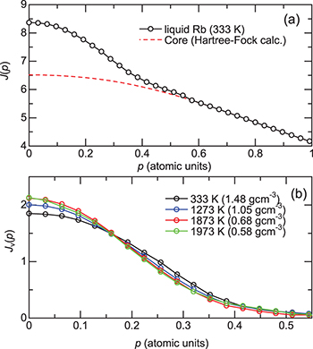
Fig. 1: (Colour online) (a) Total Compton profile of liquid Rb at 333 K and 0.1 MPa. Also shown is the profile of the core electrons in atomic Rb obtained by Hartree-Fock calculation [23]. (b) Valence Compton profiles of fluid Rb at several thermodynamic conditions. Fluid density denoted in each condition is estimated from refs. [1,30].
Download figure:
Standard imageBecause valence electrons in alkali metals are well described by the electron gas model, it is meaningful to compare the experimental valence CPs,  , with those of the electron gas model. In fig. 2(a), we compared
  with the CP of the free (non-interacting) electron gas (FEG) model,
  , and the CP of the interacting electron gas (IEG) model,
  .
.  was derived from the Fermi-Dirac distribution, where the effect of thermal broadening was included.
  was constructed from the momentum distribution n(q) given in the interpolation formulas for the numerical results of the quantum Monte Carlo method [26], where the parameters of the formula are given for several values of rs (rs is the Wigner-Seitz radius in units of the Bohr radius). The n(q) that corresponds to each experimental fluid density was derived by the linear interpolation with respect to rs from that at
  and 8 because the rs that corresponds to the experimental condition ranges from 5.4 to 7.4. Both
  and
and  at each condition were derived by the formula
  [16] and broadened by the experimental resolution. For
  , no thermal effects were included. Both CPs were then normalized to 1.
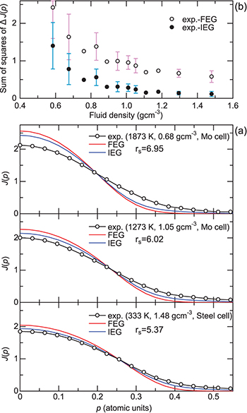
Fig. 2: (Colour online) (a) Experimental CPs at several conditions in comparison with those of the electron gas model. (b) The sums of squares of the CP difference between the experimental CP and the electron gas CPs ( and
and  ). Data points at each density are averaged over several experimental runs. The error bars indicate the sample standard deviation, which are displayed except for the densities at which only one time measurement was carried out.
Download figure:
Standard imageAn important feature exhibited in fig. 2(a) is that, irrespectively of the models of FEG and IEG, the difference between the experimental  and the theoretical ones actually increases as the fluid density decreases. Namely, the width of
  decreases more slowly than the width of
  and
and  with volume expansion. We evaluated the sum of squares of the CP difference to quantify the observed difference. Figure 2(b) shows the sum of squares plotted as a function of the fluid density. Note that the sum of squares gradually increases at approximately 1.1–1.0 g cm−3 and then increases more sharply below ≈0.8 g cm−3. These are commonly observed features in both the CP differences, although the thermal broadening effect is only considered for
  . This suggests that the effect of temperature on electrons seems to play a minor role in these tendencies of the sum of squares.
For several crystalline systems (Al, Li), it has been regarded that the effect of lattice expansion is dominant in the temperature variation of valence CPs [27]. Results consistent with this interpretation were also reported for the temperature dependence of valence CPs of Be [28]. When the experimental results are compared with those of the electron gas model for Al and Li, the inclusion of lattice expansion effects in the model reasonably explains the observed narrowing of experimental valence CPs [27]. Recent ab initio calculations examine thermal effects on CPs of disordered systems using the real-space multiple scattering Green's function formalism coupled with density functional theory molecular dynamics [29]. The results reproduce the temperature dependence of CPs experimentally observed in thermally disordered Be, Li, and Si. In our calculations based on the electron gas model, however, the atomic configurations are not taken into account and the effect of expansion is included only by the electron density derived from the (macroscopic) fluid density in the expanded state [1,30]. Hence, the enhanced discrepancy between experimental and theoretical results with volume expansion suggests that the assumption of spatially uniform expansion in the model is invalid.
As is evident in fig. 2(a),  is closer to
  than
than  at all thermodynamic conditions, which indicates that the inclusion of the interaction between electrons is necessary. Therefore, in the next section, we adopt the IEG model as the electron gas model for comparison with the experiment.
Electron kinetic energies and CP differences
An important advantage of CPs is that they can provide information on the energetics of electrons. The second moment of a CP is formally connected with the expectation value of the electron KE,  [16,31],

(This quantity gives 3/5 of the Fermi energy for the case of  normalized to 1 without the resolution broadening.) The analysis using the scaled CP difference is reported to be quite effective for discussing the energetics of electrons in ice Ih by
  [32], where relative variations from a reference thermodynamic condition provide meaningful information on the energetics of electrons, such as the configurational enthalpy [32]. The evaluation of the electron kinetic-energy difference is also quite effective as seen in recent investigations for supercooled water [33] and cathode materials of Li batteries [34]. In our analysis, the determination of the absolute values of
  was found to be difficult, after making careful examinations to clarify the effects of the core subtraction analysis (see SM). Here, we derived
  from the valence CPs of fluid Rb and evaluated its relative variation as a function of the density from the reference condition. In fact, we evaluated the KE difference defined as
  .
.
 derived from the experimental CPs is shown in fig. 3. We set the value of
  to that at 333 K (1.48 g cm−3). The density dependence of
  was found to exhibit a systematic trend as shown in the figure, even if the order of the polynomials and the pc values are varied in the core-subtraction analysis. Also shown in the figure is
  . The value of
  is that at the electron density corresponding to a fluid density of 1.48 g cm−3. As can be seen in the figure,
  appears to follow
  in the higher-density region, and the reduction of ≈0.007 hartree from 1.48 to 1.1 g cm−3 is certainly consistent with the prediction of the electron gas model; however, an appreciable upward deviation appears from
  in the lower-density region. A notable feature is that the deviation from the electron gas model already occurs in the higher-density region at approximately 1.05–1.0 g cm−3.
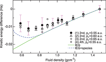
Fig. 3: (Colour online) Fluid density dependence of the experimental electron kinetic-energy difference in comparison with theoretical calculations. The energy is evaluated per electron. The energy unit is the hartree. The order (2nd or 4th) of the polynomial used to approximate the background and the cutoff momentum pc are indicated for each condition of (1)–(4). The error bars (sample standard deviation) for condition (1) are only displayed for clarity (except for the densities at which only one time measurement was carried out). The kinetic-energy difference of IEG is denoted as IEG, and that of the mixture model is denoted as IEG + species (see the text).
Download figure:
Standard image shows the large deviation from the electron gas model at lower density, where an appreciable increase in the fraction of the molecular units has been suggested [10–12]. We also calculated the
  by employing a model CP that combines the CP of the electron gas with that of the atomic or molecular species. The assumption was made that the CP can be constructed by a linear combination of the constituent CPs. For the calculation of the CP of atomic or molecular species, we used ERKALE [35], which enables the Hartree-Fock calculation of CPs using the Gaussian basis sets2
. We consulted the species indicated in ref. [10] and calculated the CPs of Rb, Rb2, and
by employing a model CP that combines the CP of the electron gas with that of the atomic or molecular species. The assumption was made that the CP can be constructed by a linear combination of the constituent CPs. For the calculation of the CP of atomic or molecular species, we used ERKALE [35], which enables the Hartree-Fock calculation of CPs using the Gaussian basis sets2
. We consulted the species indicated in ref. [10] and calculated the CPs of Rb, Rb2, and  . They were then merged with the
  by the linear combination as follows:
  . Here
  , Rb2,
  , and xi is the fraction of electrons belonging to each species given in ref. [10]. The electron density (or rs) characterizing the electron gas part,
  , was set to the value estimated from the (macroscopic) fluid density.
  and
and  were normalized to 1. The calculated CP was broadened by the experimental resolution. Then, we calculated
  from
from  . Here,
  is set to
  . In the calculation, the upper bound of the integration was set to 1.5 a.u., because almost the same dependence was reproduced above this value, indicating that the effects of the cutoff were almost excluded.
 is also shown in fig. 3. The results of the model indicate that the increase in the molecular units contributes to the enhancement of the KE. The occurrence of this upward deviation seems to qualitatively reproduce the experimental trend of
  below ≈0.8 g cm−3. In the higher-density region above ≈0.8 g cm−3,
  agrees with
  because the fraction of the molecular species is almost zero. As a result,
  also exhibits small upward deviation from the model curve below approximately 1.1 g cm−3. The result can be attributed to the fact that the width of
  is reduced more slowly with volume expansion than that of
  , as seen in fig. 2.
Figure 4(a) shows CP differences derived for experimental CPs and theoretical (IEG) CPs. A broad dip with negative value was observed around 0.2–0.3 a.u. for both  and
and  .
.  agrees well with
  at 1.30 g cm−3. However, the depth of the dip becomes more pronounced for
  than for
  as the fluid density decreases, which arises from the increasing discrepancy between the experimental CPs and the theoretical ones with volume expansion, as seen in fig. 2.
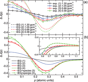
Fig. 4: (Colour online) (a) Experimental CP differences in comparison with theoretical (IEG) CP differences at several fluid densities. (b) CP differences of IEG and those of the model (IEG+species). The numbers (1)–(4) represent the conditions of the fluid density as indicated in (a). The inset shows an enlargement of CP differences in higher momentum range. The CP difference  is defined as
  .
.  denotes the CP at the reference condition. For experimental CP differences,
  is the experimental CP at 333 K (1.48 g cm−3). For the CP differences of IEG and the model,
  is the CP of IEG at the electron density evaluated for the fluid density of 1.48 g cm−3.
Download figure:
Standard imageFigure 4(b) shows a comparison between  and
and  (IEG+species).
  was calculated at densities of 0.68 g cm−3 and 0.58 g cm−3, where
  is dominant in the constituents of molecular species. The fractions of
  are approximately 0.07 and 0.21 at higher and lower densities, respectively. Although difference between
  and
and  at the same density seems quite small,
  becomes piled-up at
  and has an enhanced tail at approximately
  as indicated by the inset in fig. 4(b). As mentioned in the KE evaluation using the model, the integration range was set to 1.5 a.u. The range includes a long tail due to the species and the inclusion of the tail in the integral is found to be responsible for the enhancement of the KE given by the model.
Although the accessible momentum range is limited to about 0.6 a.u. in the experiment (see SM), it should be noted that changes in the  profile can also be seen in the
  profile in fig. 4(a), that is,
  becomes piled-up at
  and enhancement of the tail at
  , which is slightly lower than
  in
in  , is clearly observed at 1973 K (0.58 g cm−3) compared to
  at the adjacent condition of 1873 K (0.68 g cm−3). The observed changes in the
  profile are not necessarily attributed to the features of
  , but they imply the emergence of some factors that cause the electron localization similar to the molecular formation in the fluid and contribute to the enhancement of KE.
As can be understood from fig. 3, the deviation of  from that of the mixture model indicates that the experimental trend cannot be captured by a physical picture in which molecular units appear in the fluid with a finite amount of fractions. In fact, it was indicated that the extended cluster model considering the formation of a larger and fluctuating cluster would be more suitable within the density range 2–3ρc [10].
Several ab initio simulations for fluid Rb have been carried out [37–40] and transient dimer- or trimer-like atomic correlations were observed near  [37–39]. It is noteworthy that, even at a higher density of 0.97 g cm−3, an inhomogeneous electronic charge density was actually observed accompanying the spatial fluctuation of the atomic arrangement [40]. A close correlation can be envisaged between such inhomogeneity in the simulation and the observed
  deviation at the early stage of expansion (below ≈1.1 g cm−3), because the occurrence of the inhomogeneity means that the electron density is locally kept at higher values than in the case of uniform distribution.
Our results are consistent with inhomogeneous charge distributions of valence electrons found in the simulations and also support the indication that a large and fluctuating cluster is more appropriate [10] to explain the magnetic susceptibility enhancement [8,9] for densities between 2 and 3 times the critical density.
A remarkable feature is that the density range where this deviation in KE is observed shows good agreement with the region where structural changes in expanded fluid Rb start to appear (≈ 1.1 g cm−3) [13], where the nearest-neighbor distance decreases in spite of volume expansion. The observed structural features were interpreted to be due to the instability of the low-density electron gas [13]. For such structural features, a theoretical analysis was given that the interionic attractive force develops with an enhanced attraction between quasiparticles of valence electrons in low-density electron gas [14]. The observed  behavior in the relatively higher-density region below ≈1.1 g cm−3 suggests that charge inhomogeneity of valence electrons, coupled with ionic dynamics, has occurred in the fluid and a fluctuation intrinsic to the low-density electron gas causes the occurrence of such charge inhomogeneity in real fluid Rb. A recent inelastic neutron scattering investigation for fluid Rb [41] reported that the density dependence of the dynamic structure factor can be reasonably explained by the existence of metallic and non-metallic (microscopic) domains in the fluid at densities between 3 and 4 times the critical density, where the volume fraction of a metallic domain decreases and that of a non-metallic domain increases with overall density reduction. Our observation at the corresponding densities is consistent with this physical picture which suggests charge inhomogeneity in the fluid.
In summary, X-ray Compton scattering enables us to directly access the information on the electronic state in expanded fluid Rb. The results reveal intriguing features of the electronic state in the fluid, which suggests the appearance of inhomogeneous charge distribution of the valence electrons in the density range where the fluid is still metallic. The results bridge the gap between the molecular domain and the condensed-matter domain in expanded fluid Rb, and shed light on the problem of the phase separation behaviors of the low-density electron gas [42,43], metallic nature and its stability in matter under various thermodynamic conditions, such as the dilute metallic system with solvated electrons [44], or the Fermi-degenerated plasma created under extreme conditions [45].
Acknowledgments
The authors thank the late T. Fukumaru for his great contributions, and also thank the late M. Yao and Prof. K. Nagaya for valuable discussions. The authors would like to acknowledge Kobe Steel Co., Ltd., Mitsubishi Elec. Co., Ltd., and Koyo Assetsu Co., Ltd. for technical support. This work was supported by JSPS KAKENHI (Research Nos. 19204040, 24540401, and 15K05209), and the Toray Science Foundation. The synchrotron radiation experiments were performed at the BL08W of SPring-8 with the approval of JASRI (Prop. 2011A1138, 2011B1195, 2012A1195, 2012B1522, 2013B1070 and 2014A1101, and 2014B1111).

