


Abstract
We examine the local density of states (DOS) at low energies numerically and analytically for the Hubbard model in one dimension. The eigenstates represent separate spin and charge excitations with a remarkably rich structure of the local DOS in space and energy. The results predict signatures of strongly correlated excitations in the tunneling probability along finite quantum wires, such as carbon nanotubes, atomic chains or semiconductor wires in scanning tunneling spectroscopy (STS) experiments. However, the detailed signatures can only be partly explained by standard Luttinger liquid theory. In particular, we find that the effective boundary exponent can be negative in finite wires, which leads to an increase of the local DOS near the edges in contrast to the established behavior in the thermodynamic limit.
Export citation and abstract BibTeX RIS
Introduction
Interacting one-dimensional quantum wires are well-studied examples of systems in which the Fermi liquid paradigm of electron-like quasi-particles is known to break down. Luttinger liquid theory predicts that strong correlations lead to the remarkable phenomenon of separate spin- and charge-density waves as the fundamental collective excitations in one dimension at low energies [1]. Experimental confirmation for this picture has long been controversial, but now there is some evidence for separately dispersing spin and charge resonances for quantum wires on semiconductor hetero-structures [2, 3], quasi–one-dimensional crystals [4] and self-organized atomic chains [5] as a function of momentum. The density of states (DOS) has also been analyzed by scanning tunneling spectroscopy (STS) in carbon nanotubes [6–8] and self-organized atomic chains [9]. This immediately invites the question as to whether there are characteristic signatures from standing waves of separate spin and charge densities, that can potentially be detected in locally resolved STS experiments in finite wires. Detailed Luttinger liquid calculations near boundaries exist, which predict corresponding wave-like modulations in the local DOS and a sharp reduction of the DOS near boundaries [10–16]. However, it is far from clear whether these signatures are robust in realistic lattice systems, since even minimalistic models like the Hubbard chain are not perfect Luttinger liquids. There are two main reasons for possible discrepancies: First, the assumed degeneracy of spin and charge modes in the low-energy spectrum can never be exact and will be lifted by band curvature and other effects. Second, it is known that strong logarithmic corrections will arise from a spin umklapp operator which is generically present in 1D electron systems with SU(2) invariant interactions [17–19].
The most relevant minimalistic lattice model for quantum wires is the Hubbard chain,

which captures the main aspects of interacting one-dimensional electron systems. This model shows signatures of spin-charge separation in numerical simulations of the momentum resolved DOS [20], which is the central quantity relevant for photoemission experiments. In this paper we will now analyze the local DOS as a function of position and energy which in turn is relevant for STS experiments.
Recently, several numerical density matrix renormalization group (DMRG) studies considered the local DOS for spinless lattice fermion models in one dimension [21–23], where there is no spin and charge separation. Therefore, the complications mentioned above do not arise [24, 25] and the agreement with theory is close to perfect in that case. As we will show here, the local DOS for a spinful electron system away from half-filling is much more complex and some key features of the Luttinger liquid theory are strongly renormalized.
The observable of interest is the local DOS to tunnel an electron with spin up at a certain energy ω into the wire,


Here, the fermion operator ψ†↑,x creates a particle at position x on top of the ground state  and the sum runs over all states
  with one additional electron.
In the following we will compare analytic calculations for the local DOS from Luttinger liquid theory with simulations using the numerical DMRG algorithm [26, 27]. For the matrix elements in eq. (2) we use a multi-target DMRG with a large number of target states in two different particle number sectors [21] and keep track of all local fermion creation operators.
The spectrum
In order to identify the separate spin and charge excitations, we first focus on the energy spectrum Δω = ωα − ω0 for finite wires of length L as a function of interaction U as shown in fig. 1 in units of t = 1. The ground state |0〉 is assumed to be a filled Fermi sea with total magnetization Sz = 0, so that all particle excited states |ωα〉 have N↑ = N↓ + 1 particles and total spin z-component Sz = 1/2.
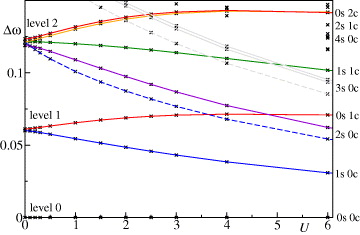
Fig. 1: (Color online) Energies Δω = ωα − ω0 as a function of U for excited states with N↑ = N↓ + 1 = 31 particles on a lattice of length L = 90. The quantum numbers on the right indicate the corresponding mode {ms,mc}. Dashed lines correspond to S = 3/2 states. For larger U, excitations from level 3 (3s 0c) and level 4 also appear in the low-energy spectrum.
Download figure:
Standard imageFor U = 0 all excitations are described by simple products of fermion operators  , where
  and |ω0〉 = c†↑,0|0〉 is the lowest-energy particle excitation. Since the spectrum is approximately linear Δω ∼ vF
(k − kF
), a state involving several fermion operators (i.e., a multi-particle excitation) is nearly degenerate with a single-particle excitation at U = 0 if the sum of excited wave numbers is the same, which results in the quantized fermion levels shown in fig. 1. For example, in level 1, the two states c†↑,1|0〉 and c†↑,0c†↓,0c
↓,−1|0〉 both have approximately the same energy ω1 − ω0 ≈ vF
k1. In general there are many multi-particle states in each level n, but only one single-particle state c†↑,n|0〉 carries all the DOS if U = 0.
and |ω0〉 = c†↑,0|0〉 is the lowest-energy particle excitation. Since the spectrum is approximately linear Δω ∼ vF
(k − kF
), a state involving several fermion operators (i.e., a multi-particle excitation) is nearly degenerate with a single-particle excitation at U = 0 if the sum of excited wave numbers is the same, which results in the quantized fermion levels shown in fig. 1. For example, in level 1, the two states c†↑,1|0〉 and c†↑,0c†↓,0c
↓,−1|0〉 both have approximately the same energy ω1 − ω0 ≈ vF
k1. In general there are many multi-particle states in each level n, but only one single-particle state c†↑,n|0〉 carries all the DOS if U = 0.
The situation changes for finite U. Now all states may potentially carry spectral weight in the DOS and the near-degeneracy of the levels is lifted. According to the Luttinger liquid picture the states are now described by integer spin and charge quantum numbers {ms,mc} with energies  in terms of the spin and charge velocities vs ⩽ vc [1, 14]. The spectrum in fig. 1 shows a regular spin and charge spacing with quantum numbers shown on the right. For each spin/charge mode {ms,mc} there can be several states with approximately the same energy. The number of states in each mode is given by the number of ways it can be created by boson creation operators b†m,ν, i.e., the product of the integer partitions of ms and mc. For example, for the mode 0s 2c in fig. 1, we have mc = 2 = 1 + 1 corresponding to the two states created by b†2,c and (b†1,c)2, respectively, which indeed have almost the same energy. On the other hand, the near-degeneracies of spin modes (e.g., 2s 0c) are significantly split in fig. 1 by well-known logarithmic corrections as will be discussed below [17–19].
Regarding the DOS, it is now interesting to explore how the total spectral weight is distributed among the excited states. The compact answer from Luttinger liquid theory is that the summed up DOS in each mode {ms,mc} should be proportional to a power law of the corresponding energy, but there are no predictions how the DOS is distributed among the states within each mode. For the lowest-energy modes the situation is still simple, since the first level corresponds to one spin and one charge state, which should have roughly the same DOS of 1/2 each for small U according to theory. However, the numerical results in fig. 2 already demonstrate obvious deviations from this prediction, since the charge mode has a much larger DOS for small U. The reason for this discrepancy comes from the non-linear band curvature, which lifts the degeneracy for finite L even at U = 0, so that the interaction has to overcome this energy splitting. Indeed for cases in which the two states are exactly degenerate at U = 0 (e.g., in the thermodynamic limit) the spin and charge states have comparable DOS even for infinitesimally small U. As can be seen in fig. 2 for L = 90 the charge state dominates for U ≲ 0.5, which would imply that for  the band curvature is dominant over the interaction effects. The next five states from the second fermion level in fig. 2 show a similar crossover behavior with U. Nonetheless, features in the local DOS will clearly show the interaction effects even in the crossover region as we will see below.
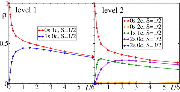
Fig. 2: (Color online) Total DOS for the excitations of the first two levels from fig. 1.
Download figure:
Standard imageIn the 0s 2c and the 2s 0c modes there are two states each as expected. However, only one of the states in each mode contributes most of the corresponding DOS, while the other state would be practically invisible in an STS experiment. The reason why some states in a given mode have zero DOS can sometimes be linked to exact symmetries, such as the SU(2) symmetry of generic Coulomb interactions. In particular, all particle excitations |ωα〉 in the Sz = 1/2 sector are representatives of SU(2) multiplets. The lowest-energy state |ω0〉 always belongs to a doublet with S = 1/2. Excitations with charge bosons b†ℓ,c never change the total spin, but excitations with spin bosons b†ℓ,s may generate higher spin values, which can be calculated using the commutation rules of the non-Abelian SU(2)-Kac-Moody algebra [17], since the spin bosons correspond to the modes of the SU(2) current along the z-direction as discussed in the appendix. For example the lowest-energy S = 3/2 state is given by the spin boson excitation ![$\frac {1}{\sqrt {3}}[(b^\dagger _{1,s})^2 - b^\dagger _{2,s}] |\omega _0\rangle $](https://content.cld.iop.org/journals/0295-5075/101/5/56006/revision1/epl15277ieqn7.gif) with ms = 2 which is plotted as a dashed line in fig. 1. The total spin analysis is discussed in more detail in the appendix. It is useful since states with S > 1/2 must have zero DOS due to angular momentum addition rules. For example in the fifth spin mode 5s 0c, there are 7 states, three of which have total spin S = 3/2 and exactly zero DOS. Interestingly, three more states carry only very small spectral weight, so that only one state dominates for this mode. This indicates that the eigenstates remain the same in terms of their bosonic expressions even for U ≠ 0. For charge modes there is also exactly one state which carries the overwhelming weight in each mode, but the DOS of the other states is finite and generally increases with U.
with ms = 2 which is plotted as a dashed line in fig. 1. The total spin analysis is discussed in more detail in the appendix. It is useful since states with S > 1/2 must have zero DOS due to angular momentum addition rules. For example in the fifth spin mode 5s 0c, there are 7 states, three of which have total spin S = 3/2 and exactly zero DOS. Interestingly, three more states carry only very small spectral weight, so that only one state dominates for this mode. This indicates that the eigenstates remain the same in terms of their bosonic expressions even for U ≠ 0. For charge modes there is also exactly one state which carries the overwhelming weight in each mode, but the DOS of the other states is finite and generally increases with U.
Local density of states
For a complete analysis it is now useful to turn to the local DOS ρms,mc(x) for each mode {ms,mc}. For a non-interacting system, the local DOS is given by the square of a quickly oscillating standing wave, corresponding to the eigenstate at the corresponding wave vector near kF . However, with interactions we also expect long-wavelength modulations and a characteristic behavior near the boundary. It is therefore useful to decompose the local DOS into a quickly oscillating part (o) and a uniform part (u). In order to analyze the long-wavelength modulations we will concentrate on the uniform part of the local DOS in the following, which according to bosonization is given by a product of spin and charge contributions [14]

for a given mode {ms,mc}. The slowly varying amplitudes ρuν,m(x) can be determined by a simple recursive formula for spin and charge (ν = c,s) separately [14],
where

Here we have defined spin and charge exponents aν = (1/Kν + Kν)/4 and bν = (1/Kν − Kν)/4 in terms of the respective Luttinger parameters Kν for ν = c,s. The overall prefactor  in eq. (4) does not depend on energy and serves as normalization so that ρuν,m=0 = 1. It is straightforward to see that the recursive formula results in power laws for the DOS in the bulk ρ∝ωac+as−1 for L → ∞ [14, 28]. In addition, the formula predicts slow wave-like modulations in the local DOS due to the second term in eq. (6), which also survive in the thermodynamic limit near the edge [10].
The local DOS from the DMRG data is shown in fig. 3 for the first few modes at 1/3-filling. For the lowest excitation |ω0〉 the oscillating and uniform parts are the same and given by the prefactor |c(x)|2. Already at first sight it is surprising to see that the local DOS for all modes increases slightly near the boundary, while all previous analytic calculations have predicted it to decrease according to the boundary exponent [10, 28, 29]. Indeed it must be emphasized that the local DOS does not fit the theoretical prediction. All curves should in principle be fit free, up to one overall normalization, since the local DOS of all levels follows from eqs. (4)–(6), where the Luttinger parameters Kc(U) and Ks = 1 are known from the thermodynamic Bethe ansatz. However, in fig. 3 two important adjustments have been made: First the theoretical curves were shifted down for the charge modes and up for the spin modes in order to fit the numerical data (indicated by arrows). This adjustment was already observed in the crossover of the total DOS in fig. 2 due to the competition of energy scales (band curvature vs. interaction) as argued above. We could not find any explanation of the shifts in the framework of a renormalized Luttinger liquid. Secondly, we find that the spin Luttinger liquid parameter must be chosen considerably larger than unity Ks ≈ 1.16 for all spin modes in order to fit the numerical data corresponding to attractive behavior in the spin modes. This is especially surprising since the charge Luttinger parameter from the Bethe ansatz Kc = 0.9081 agrees perfectly with the data without any finite-size adjustments. There are no other adjustable parameters in the fits of fig. 3, except for one overall normalization constant. The oscillating parts ρoν can be analyzed analogously and give the same results (not shown). The local DOS can also be calculated by Fourier transforming the real-space Green's function [10–13, 28], but for an analytic analysis of individual states the recursive formulas in eqs. (4)–(6) are a great advantage, since they give a closed form without divergences and in return allow the quick and accurate determination of the effective parameters Ks and Kc by fitting the data from (numerical) experiments for the first spin and charge excited states.
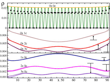
Fig. 3: (Color online) The local DOS of the first few modes for L = 92 and U = 1. Points are DMRG data and lines are theoretical predictions for Kc = 0.9081 and Ks = 1.16 adjusted by a shift as indicated by arrows (see text). Top: local DOS for |ω0〉. The thick line corresponds to 2|cx|2. Lower plots: uniform part of the local DOS for the first few charge and spin modes.
Download figure:
Standard imageIn fig. 4 the behavior of the Luttinger parameters from the corresponding fits to the uniform local DOS is shown as a function of interaction and length at 1/3-filling. The charge parameter from the Bethe ansatz Kc always agrees very well with the data without any additional adjustments. However, the observed spin parameter Ks is considerably larger than Ks = 1. Non-Abelian bosonization predicts Ks = 1 for any SU(2) invariant model, but at the same time it is known that a marginal irrelevant operator causes corrections to the anomalous dimension which only vanish logarithmically slowly with 1/ln L in the thermodynamic limit [17, 18]. In Abelian bosonization such a correction can indeed effectively be modeled by a renormalizing spin Luttinger parameter [17–19, 30, 31]

where L0 is non-universal and depends on the model and the quantity of interest. As shown in fig. 4 such a renormalization description is indeed consistent with our data for Ks. The parameter Ks increases with U at a given length L, but decreases slowly as the length is increased. The parameter Ks appears to be the same for all spin modes at a given U and L, i.e., independent of energy ω. The renormalization of Ks is very slow, so that exponentially large systems are required to observe the thermodynamic limit Ks → 1. The fit parameters for Ks ≈ 1 + 1.98g with ln L0 ≈ −6 are outside the range, which would normally be expected for a spin chain model [19]. Therefore, the particular form of the observed corrections remains a puzzle.
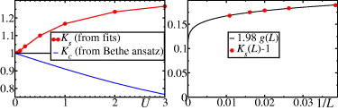
Fig. 4: (Color online) Left: Luttinger parameters Kc (line) from the Bethe ansatz and Ks (points) from the fits to ρus,m=1(x) as a function of U for L = 92. Right: renormalization of Ks (points) at U = 1 with the system size L compared to eq. (7).
Download figure:
Standard imageNonetheless, the results of the logarithmic corrections have interesting consequences. In particular, the corrections are so large, that the boundary exponent αB = (1/Ks + 1/Kc)/2 − 1 may become negative if Ks + Kc < 2KsKc, i.e., Ks − 1 ≳ 1 − Kc to lowest order in the correction, which is indeed the case for small U ≲ 2t at L = 92. This results in an increase of the local DOS for small energies ω and small distances x near the boundary, which is described by a weak power law divergence ρ∝xbs+bcωαB. Such a negative boundary exponent would also explain the recently reported boundary anomalies for small interactions in functional renormalization group studies [32, 33]. It is known that logarithmic corrections also exist as a function of energy near the boundary, which lead to a very small energy region where an uncorrected boundary exponent can be observed [24, 25].
Conclusions
In conclusion, we have analyzed the local DOS of the Hubbard model in the low-energy regime. Individual states can be classified by separate spin and charge quantum numbers. We observe that typically only one eigenstate has a relatively large local DOS in each spin/charge mode, while all other states in that mode are negligible. The spin and charge Luttinger parameters Ks and Kc can be extracted from the modulations in the local DOS of individual excited states. While the charge parameter Kc agrees well with the Bethe ansatz, the spin Luttinger liquid parameter is attractive Ks > 1 due to large finite-size corrections, which can only be neglected for exponentially large chain lengths. In fact, the corrections to Ks are unexpectedly strong and may even lead to negative boundary exponents for moderate interactions U ≲ 2t. The common assumption that it is possible to generically use Ks = 1 due to SU(2) invariance is certainly not justified for the local DOS. In particular, for finite wires on conducting substrates the interactions may be reduced by screening, so that the charge Luttinger liquid parameter Kc may be close to unity, while the spin Luttinger liquid parameters Ks can already be significantly increased, which leads to a negative boundary exponent. This would have quite dramatic consequences, since the DOS near the boundary determines the tunneling between connected wires and the renormalization of the conductivity through impurities [29], which will show an increase at low temperatures in this scenario.
Acknowledgments
We are thankful for useful discussions with A. Struck and M. Bortz. This work was supported by the DFG and the State of Rheinland-Pfalz via the SFB/Transregio 49 and the MAINZ graduate school of excellence.
Appendix:: quantum numbers from non-Abelian bosonization
In order to determine the total spin eigenstates as shown in tables 1 and 2, it is useful to use non-Abelian bosonization in the spin channel [17]. In this case the excitations are created by the modes of SU(2) currents Jam with a = x,y,z obeying the Kac-Moody algebra,

The ground state is characterized by Jam|ω0〉 = 0, ∀ m < 0. The total spin operator is given in terms of the m = 0 currents,

where
J± = Jx ± iJy. The current modes in the z-direction are related to the Abelian spin bosons above by  and
and  for m > 0. It is therefore straightforward to consider the total spin of any bosonic spin and charge excitation by using the Kac-Moody commutation relations. The charge bosons commute with the total spin operator S2. Spin excitations are created by products of spin creation operators b†m,s acting on |ω0〉. The corresponding normalized states can be labelled by the set of which bosons were created |{m1,m2,m3,...}〉, e.g.,
  . Therefore, the matrix elements of 〈{m1,m2,m3,...}|S2|{m1',m2',m3',...}〉 between any two such excitations can be evaluated uniquely by the Kac Moody algebra (A.1). The Jz0 operators commute with all excitations and the ground state is characterized by
  in our case. For the J± operators we use the Kac-Moody relation in eq. (A.1) with the help of computer algebra in order to successively commute them to the right until the action on the ground state is known. This results in a non-diagonal matrix for S2 for each spin mode separately, which can be brought into diagonal form. The resulting eigenstates and eigenvalues are given in table 1 for the case in which the state |ω0〉 has total spin of S = 0. In this paper we considered an excitation on the filled Fermi sea, which will correspond to a state |ω0〉 with S = 1/2. In this case the eigenstates are given in table 2.
Table 1:. The SU(2) eigenstates in terms of bosonic quantum numbers with integer spin.
| S=0 |  |
|---|---|
| S=1 |
 |
| S=0 |  |
| S=1 |
 |
| S=0 |
 |
| S=1 |
 |
| S=1 |
 |
| S=0 |
 |
| S=0 |
 |
| S=1 |
 |
| S=1 |
 |
| S=2 |
 |
| S=0 |
 |
| S=0 |
 |
| S=1 |
 |
| S=1 |
 |
| S=1 |
 |
| S=1 |
 |
| S=2 |
 |
Table 2:. The SU(2) eigenstates in terms of bosonic quantum numbers with half-integer spin.
| S=1/2 | 
|
|---|---|
| S=1/2 |

|
| S=1/2 |
 |
| S=3/2 |
 |
| S=1/2 |
 |
| S=1/2 |
 |
| S=3/2 |
 |
| S=1/2 |  |
| S=1/2 |
 |
| S=1/2 |
 |
| S=3/2 |
 |
| S=3/2 |
 |