

- EAER>
- Journal Archive>
- Contents>
- articleView
Contents
Citation
| No | Title |
|---|---|
| 1 | Gambling to Preserve Price (and Fiscal) Stability / 2024 / IMF Economic Review / vol.72, no.1, pp.32 / |
Article View
East Asian Economic Review Vol. 24, No. 4, 2020. pp. 417-440.
DOI https://dx.doi.org/10.11644/KIEP.EAER.2020.24.4.386
Number of citation : 1View
69
Download
60
Financing COVID-19 Deficits in Fiscally Dominant Economies: Is The Monetarist Arithmetic Unpleasant?

Abstract
The coronavirus pandemic of 2019-20 confronted fiscally dominant regimes around the world with the question of whether the large deficits caused by the health crisis should be monetized or financed by issuing debt. The unpleasant monetarist arithmetic of Sargent and Wallace (1981) states that in a fiscally dominant regime tighter money now can cause higher inflation in the future. In spite of the qualifier ‘unpleasant,’ this result is positive in nature, and, therefore, void of normative content. I analyze conditions under which it is optimal in a welfare sense for the central bank to delay inflation by issuing debt to finance part of the fiscal deficit. The analysis is conducted in the context of a model in which the aforementioned monetarist arithmetic holds, in the sense that if the government finds it optimal to delay inflation, it does so knowing that it would result in higher inflation in the future. The central result of the paper is that delaying inflation is optimal when the fiscal deficit is expected to decline over time.
JEL Classification: E52, E61, E63
Keywords
Optimal Monetary Policy, Inflation Tax, Fiscal Deficits, Public Debt
I. INTRODUCTION
In “Some Unpleasant Monetarist Arithmetic,” Sargent and Wallace (1981) warned that ‘tighter money now can mean higher inflation eventually.’ They derived this conclusion in the context of a model with a policy regime characterized by fiscal dominance. Specifically, in their formulation the fiscal authority sets an exogenous path for real primary deficits, which must be passively finance by either printing money or issuing debt. In this environment, tightening current monetary conditions requires increasing the growth of interest-bearing debt. Because the government must pay its debts eventually, at some point it has to increase the money supply to pay not only for the primary deficits but also for the increase debt and accumulated interest, entailing higher inflation than if it had not tightened monetary conditions.
The fiscally dominant regime studied by Sargent and Wallace is a realistic description of the restrictions that central banks around the world have faced at different points in history. The most recent example is the burst of fiscal deficits caused by the covid-19 pandemic of 2020. Lock downs caused a collapse in tax revenue and a burst in government transfers and health-related government spending. A case in point from the pre-pandemic era is Argentina since the beginning of the Macri administration in late 2015. The government inherited a large fiscal deficit of about 5 percent of GDP and was quite limited in its ability to either cut spending or raise taxes. As a result, the fiscal authority adopted a gradual approach to reducing the deficit, quite independently of the monetary stance. The central bank chose not to fully monetize the fiscal deficit. This approach gave rise to a burst of central bank debt, known, in the local jargon, as quasi-fiscal deficits. The rise in central bank debt was the subject of much criticism by orthodox economist, who, on precisely the grounds laid out by Sargent and Wallace, warn about its consequences for future inflation.
I address the question of under what circumstances, if any, postponing inflation by failing to fully monetize the fiscal deficit can indeed be the optimal policy choice. This question is relevant not only because, as the above examples testifies, we do observe policymakers in fiscally dominant regimes resorting to debt issuance to finance fiscal deficits, but also because the term ‘unpleasant’ in the monetarist arithmetic Sargent and Wallace refer to ought not to be necessarily understood as meaning ‘welfare reducing.’ In fact, Sargent’s and Wallace’s analysis is purely positive and therefore void of explicit normative predictions. This paper extends their contribution by placing the choices of their passive monetary authority in a welfare framework. Specifically, I ask what is the welfare maximizing monetary policy in a fiscally dominant regime.
To ensure that the present analysis is conducted in a level playing field with that of Sargent and Wallace, I build a model in which the unpleasant monetarist arithmetic holds. In particular, in the model, the fiscal authority sets an exogenous path for the primary fiscal deficit, and the central bank is limited to choosing the mix of money creation and debt issuance. In this model, failing to monetize the fiscal deficit does result in higher inflation eventually, exactly as dictated by the unpleasant monetarist arithmetic. The key departure from the analysis of Sargent and Wallace is that the central bank chooses a monetary policy that maximizes the lifetime utility of the representative household.
The central result of this paper is that whether or not in a fiscally dominant regime it is optimal to delay inflation by issuing debt depends crucially on the expected path of fiscal deficits. If fiscal deficits are expected to follow a declining path, or, more generally, are temporarily high—as is likely to be the case for those taking place during the coronavirus pandemic—then it may be optimal for the central bank to fall short of full monetization of the fiscal deficit. In this case, public debt will initially rise and long-run inflation will be higher than if the central bank had refrained from initially restricting the pace of monetary expansion. If fiscal deficits are expected to grow over time, or, more generally, if fiscal deficits are temporarily low, it may indeed be optimal for the central bank to follow a monetary policy that is looser than the full monetization of the fiscal deficit would require. In this case, the long-run rate of inflation is lower than under the policy of monetizing the deficits period by period. Full monetization of the fiscal deficit emerges as the optimal policy outcome when the fiscal deficit is expected to be stable over time.
The intuition behind this result is as follows. In virtually all existing monetary models, inflation represents a distortion. Smoothing this distortion over time can be welfare increasing. In this case, the central bank will tend to set a smooth path of inflation subject to the restriction that the associated present discounted value of seignorage revenues be large enough to cover the lifetime liabilities of the government. Thus, the optimal inflation rate is dictated by the average fiscal deficit, rather than by the current one. As a result, if the current fiscal deficit is above its average value, seignorage will fall short of the fiscal deficit, and the government will need to issue debt to close the gap. This expansion in government liabilities implies higher future inflation than the alternative of printing money today to pay for the entire current fiscal deficit—the monetarist arithmetic—but is preferable because it renders a smoother path for the inflation tax.
This paper is related to a large literature aimed at understanding the role of monetary policy in fiscally dominant regimes. The primary motivation of the paper stems from the work of Sargent and Wallace (1981). The key result of the paper that if the expected path of primary deficts is decreasing the optimal monetary-fiscal regime calls for a flat rate of inflation and debt financing in the initial transitiion is reminicent of the tax smoothing result of Barro (1979) and Lucas and Stokey (1983). The paper is also related to papers in the tradition of the fiscal theory of the price level (Woodford, 1996; Sims, 1994; and Leeper, 1991). The key difference with this body of work is that in the present paper the government is assumed to be benevolent and to be able to commit not to allow the price level to jumpt. Thus, the present paper can be interpreted as providing a fiscal theory of the inflation rate, rather than of the price level. Manuelli and Vizcaino (2017) extend the analysis in the present paper by considering a government that lacks commitment.
The remainder of the paper is organized as follows. Section 2 presents an intertemporal model in which a demand for money is motivated by assuming that real balances produce utility. Section 3 characterizes the Ramsey equilibrium. Section 4 derives conditions under which it is optimal for the central bank to increase public debt instead of fully monetizing the fiscal deficit. Section 5 analyzes an economy with long-run growth. Section 6 provides a numerical example motivated by the Argentine 2016-2019 stabilization effort. Section 7 provides concluding remarks.
II. THE MODEL
The theoretical environment is an infinite-horizon, flexible-price, endowment economy with money in the utility function. The fiscal authority runs an exogenous stream of real primary fiscal deficits and finances them by a combination of debt issuance and money creation.
1. Households
Consider an economy populated by a large number of identical households with preferences for consumption and real money balances described by the following lifetime utility function

where
Households are endowed with an exogenous and constant stream of goods denoted

where a dot over a variable denotes its time derivative. Dividing through by the price level, one can write the flow budget constraint as

where  denotes the rate of inflation. Now letting
denote real financial wealth and
denote the real interest rate, one can express the flow budget constraint as

The right-hand side of constraint (2) represents the sources of income, given by the sum of nonfinancial income,  Households are also subject to the following terminal borrowing constraint that prevents them from engaging in Ponzi schemes

where 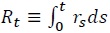 is the compounded interest rate from time 0 to time
The household chooses time paths {


and

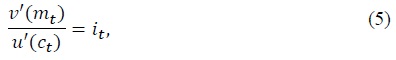
The first condition says that in the optimal plan the marginal utility of consumption must equal the shadow value of wealth. The second condition is a demand for money. It says that the desired level of real money holdings is decreasing in the nominal interest rate and increasing in consumption. Solving that optimality condition for

where
2. The Government
I assume that the primary fiscal deficit,  or issue interestbearing bonds,
  The flow budget constraint of the government is therefore given by

We can write this constraint in real terms as

This expression says that the government uses increases in its total liabilities,  and seignorage,
3. Competitive Equilibrium
Combining the flow budget constraints of the household and the central bank (equations (2) and (10), respectively) yields the resource constraint

which implies that consumption is constant over time. In turn, this result and equation (9) imply that in equilibrium the demand for money is given by
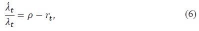
Combining (4), (6), and (11) yields
This expression says that in the present economy the equilibrium real interest rate is equal to the subjective discount factor.
Finally, the transversality condition (8) and the flow budget constraint of the government (10) are equivalent to the following intertemporal restriction

where we are using the equilibrium conditions
I am interested in economies in which the government is initially a net debtor and in which the fiscal authority runs a stream of primary deficits that is positive in present discounted value. Accordingly, we assume that


These assumptions ensure that the central bank must generate a stream of seignorage income that is positive in present discounted value to meet its lifetime financial obligations. The question is what part of its obligations should it finance with seignorage and what part by issuing debt at any point in time.
1)The present study is not concerned with dynamics in which the economy falls into liquidity traps, so I need not impose weaker assumptions on
2)Throughout this paper, I use the term seignorage revenue indistinctly to refer to
III. RAMSEY OPTIMAL CENTRAL BANK POLICY
I assume that the central bank is benevolent and has the ability to commit to its promises. This means that among all the interest rate paths and initial price levels that are consistent with a competitive equilibrium, the monetary authority picks the one that maximizes the representative household’s lifetime welfare. I refer to such equilibrium as the Ramsey optimal equilibrium. In equilibrium, welfare is given by the following indirect lifetime utility function:

Because
The optimality conditions associated with the Ramsey problem are equation (12) and

where
at all times 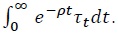 This implication is intuitive, the larger the present value of all government liabilities, the larger the amount of seignorage the central bank must generate to meet its obligations.
Because both the Ramsey optimal nominal interest rate and the equilibrium real interest rate are constant, we have that the Ramsey optimal inflation rate is also constant. Letting
for all
for all
IV. OPTIMAL PUBLIC DEBT DYNAMICS
We are now equipped with the necessary elements to characterize the optimal path of public debt,  and that

with the initial condition  and seignorage,
The optimal dynamics of public debt depend crucially on the expected future path of fiscal deficits. To see this, consider first a situation in which the primary fiscal deficit is expected to fall over time. To fix ideas, assume that the fiscal deficit evolves according to a first-order autoregressive process of the type

with

Because

Using equation (12) one can show that the expression within square brackets is zero,

which eliminates the unstable branch of the solution. It follows that the optimal equilibrium dynamics of public debt is given by

Equation (20) delivers the main result of this paper, namely, that if the fiscal deficit is expected to fall over time, it is optimal for the government to finance it partly by issuing debt, instead of by money creation alone. This result is quite intuitive. The central bank finds it optimal to smooth seignorage revenue over time. As a result, if initially the fiscal deficit exceeds seignorage revenue, the government finances the difference by issuing new debt. Over time, the primary deficits fall, but interest obligations increase. On net, however, the sum of these two sources of outlays fall, converging to zero asymptotically. In the limit, the primary fiscal deficit is nil
It is straightforward to show that if the primary fiscal deficit is temporarily low or follows an increasing path over time, as in the autoregressive form

with  and
and
For more general laws of motion of the primary fiscal deficit, one can establish that the optimal path of public debt depends on the expected trajectory of the present discounted value of future primary fiscal deficits. To see this, multiply the expression  (which is equation (17) evaluated at time

This expression says that debt will increase, decrease, or stay constant over time depending on whether the present discounted value of future primary fiscal deficits is expected to fall, increase, or stay constant over time, respectively.
3)The implementation of the Ramsey optimal plan, if unanticipated, in general gives rise to a portfolio recomposition at time 0, because households may change their desired money holdings (and therefore decrease their desired bond holdings) in a discrete fashion.
V. A GROWING ECONOMY
Thus far, I have limited the analysis to a stationary economy. It is of interest to ascertain how the conditions under which it is optimal to delay inflation change in an environment with long-run growth. To this end, here I generalize the law of motion of the endowment to allow for secular growth as follows,
where

where
Let  be the detrended version of
 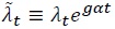 be the detrended version of

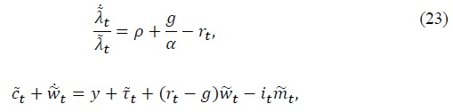

Similarly, after expressing variables in detrended form, the government flow budget constraint (10) becomes

In equilibrium, detrended consumption must equal detrended output

This result together with optimality conditions (22) and (23) implies that the real interest rate is constant and given by

According to this expression, the real interest rate is higher in the growing economy. This is intuitive, because growth makes the marginal utility of consumption fall faster over time, causing agents to demand higher compensation for sacrificing current consumption in exchange for future consumption.
By an analysis similar to that applied in the economy without growth, we can deduce that a competitive equilibrium in the economy with long-run growth is an initial price level

given the initial level of nominal government liabilities 
With long-run growth, the indirect utility function (15) takes the form

A Ramsey optimal equilibrium in the growing economy is then a path for the nominal interest rate { The first-order condition with respect to
Finally, assume, as we did in the stationary economy, that the primary fiscal deficit obeys law of motion

with  and
and

which says that if the detrended primary fiscal deficit is expected to fall over time, then it is optimal for the government not to fully monetize the fiscal deficit and instead allow the public debt to grow over time as a fraction of output. We therefore conclude that the central result of this paper is robust to allowing for secular growth.
VI. AN APPLICATION: FISCAL GRADUALISM IN ARGENTINA 2016-2019
To illustrate the implications of optimal policy for the dynamics of public debt, consider the following numerical example, motivated by developments in Argentina over the period 2016-2019. The time unit is a year. The Argentine fiscal authority inherited a large fiscal deficit of about 5 percentage points of GDP at the end of 2015. Thus, I set the initial condition
I set the initial total government liabilities equal to 38.9 percent of GDP, or4

I assume a money demand function of the form
where
Finally, I set the growth-adjusted subjective discount factor  to 4 percent, or
  and the long-run growth rate of output per capita at 2 percent, or
Under this calibration, the model predicts an optimal inflation rate of 4.8 percent per year (
Evaluating equation (20) at the parameter values given in table 0, one can trace out the path of public debt under the Ramsey optimal policy. Panel (b) of figure 0 displays the equilibrium dynamics of  is 6.5 percent of GDP, whereas seignorage revenue,
Figure 2 displays the accumulated public debt up to year 8 and the rate of inflation under the optimal monetary policy as functions of the half life of the primary fiscal deficit (top panel) and of the initial primary fiscal deficit (bottom panel). The optimal accumulation of debt is a nonmonotonic function of the half life of the fiscal deficit taking the value 0 when the half life is 0 or infinity. This is intuitive. If the fiscal deficit lasts for an infinitesimal period of time, it has no budgetary consequences, and therefore requires no financing. At the other extreme, if the deficit is infinitely lived, then the optimal policy is to generate a constant path of inflation that generates enough seignorage to finance the entire fiscal deficit. Since in this case the resulting optimal inflation rate is constant, it requires no smoothing through debt creation. In between these two extremes, positive debt accumulation is optimal. The maximum debt accumulation occurs at a half life of the deficit of 11 years, and the associated debt accumulation is 24 percent of output. The optimal inflation rate is highly sensitive to changes in the half life of the deficit, increasing from 2 percent to 25 percent as the half life increases from 0 to 30. Naturally, as shown by the bottom panels of figure 1, both optimal debt accumulation and the optimal rate of inflation are strictly increasing in the initial magnitude of the fiscal deficit,
1. Optimal Policy Versus Full Monetization
It is of interest to compare the Ramsey optimal dynamics with those implied by a monetary policy that, through money creation, keeps total government liabilities from growing over time,  I refer to this policy as full monetization of the fiscal deficit. This is the policy that results from interpreting the adjective ‘unpleasant’ attached to the monetarist arithmetic as meaning that in a fiscally dominant regime it is counterproductive to delay inflation by financing the fiscal deficit with debt. Formally, setting
  we can rewrite the central bank’s flow budget constraint (24) as

According to equation (27), under full monetization the government pays for the primary fiscal deficit and interest on its outstanding liabilities with seignorage revenue as they accrue. Using the assumed functional form for

Since
Figure 3 displays with solid lines the equilibrium dynamics of debt, inflation, and money holdings under full monetization. For comparison, the figure also displays with dashed lines the Ramsey optimal dynamics. Under full monetization, initially the central bank must generate large seignorage revenues to finance the elevated primary deficit. This results in a high initial inflation rate of 58 percent per year, more than ten times as high as the Ramsey optimal rate of inflation of 4.8 percent (panel (c) of figure 3). Because under full monetization the central bank prints money instead of issuing debt to pay for both the primary deficit and the interest on the government’s outstanding liabilities, the path of interest-bearing debt stays relatively flat at about 28 percent of GDP (panel (b) of figure 3).6 By contrast, under the Ramsey policy debt increases continuously, reaching 42 percent of output in the long run.7 As a result, in the long run, the inflation tax necessary to pay the interest on the debt is lower under full monetization than under the optimal policy. The long-run inflation rate is 2.6 percent under full monetization versus 4.8 percent under the optimal policy. This shows that the monetarist arithmetic is at work: the Ramsey policy delivers a lower rate of inflation than full monetization in the short run, but a higher one in the long run. However, in this case the monetarist arithmetic is not unpleasant. Panel (d) of figure 3 shows why. Under the Ramsey policy real money balances display a much smoother pattern than under full monetization. Because the period utility function is concave in real money balances, households prefer the smoother path of money.
4)This figure is composed of treasury liabilities with the private sector of 22.9 percent of GDP and central bank liabilities with the private sector of 16 percent of GDP at the beginning of 2016. I calculate the liabilities of the treasury with the private sector as the difference between the total debt of the treasury of 53.6 percent of GDP and the debt of the treasury with other government agencies of 30.7 percent of GDP (Informe Ministerio de Hacienda y Finanzas, first quarter 2016). I measure the liabilities of the central bank with the private sector by the sum of the monetary base and the stock of Lebac bonds outstanding. These two aggregates stood at 600 billion pesos and 360 billion pesos, respectively, at the beginning of 2016 (Informe Diario del BCRA, 2016). At the beginning of 2016, Annual GDP in Argentina was estimated to be about 400 billion dollars, and the nominal exchange fluctuated around 15 pesos per dollar. Taken together, these figures imply liabilities of the central bank of 16 percent of GDP.
5)The interest-rate semielasticity of the demand for money is defined as
6)Indeed
7)At time 0, debt is higher under full monetization than under the Ramsey policy (panel (b) of
VII. CONCLUDING REMARKS
The coronavirus pandemic of 2019-2020 has led to an unprecedented burst of fiscal deficits around the world, as tax revenue collapsed and transfers and health-related expenditures soared. In countries with monetary dominance, this situation causes the expectation of future increases in taxes and cuts in government spending, with monetary policy going about its business of maintaining price stability and full employment. By contrast, in economies in which the policy regime is fiscally dominant, policymakers are confronted with the question of how much of the fiscal imbalances they should monetize and how much they should finance with public debt. In other words, these governments must negotiate a tradeoff between current and future inflation. The resolution of this tradeoff is the central focus of the present investigation.
In a fiscally dominant economy, a central bank that commits not to let the price level jump does not control the average level of inflation. This is because under this policy regime money creation must passively finance the present discounted value of fiscal deficits plus the government’s initial liabilities. By controlling when to print money, the central bank can, however, choose the time distribution of inflation. The unpleasant monetarist arithmetic states that tight current monetary conditions imply higher inflation in the future. This paper does not quarrel with this dictum, but with the conclusion—implicit in the qualifier ’unpleasant’—that in a fiscally dominant regime tight monetary policy, understood as financing part of the fiscal deficit by issuing debt, is undesirable. Arriving at such a conclusion requires a normative analysis. In this paper I attempt to fill this gap, by characterizing the welfare maximizing path of public debt in a monetary economy characterized by fiscal dominance.
The main result derived from this analysis is that in a fiscally dominant regime tight money may not have unpleasant consequences, but, on the contrary, be optimal. This result obtains when the fiscal deficit is expected to fall over time or is temporarily high. The fiscal imbalances observed during the covid-19 pandemic clearly fit this description. The intuition is simple. Among all the inflation paths that generate enough seignorage revenue to pay for the present discounted value of the government’s liabilities, the monetary authority prefers a flat one to smooth out the distortions created by the inflation tax. In turn, a flat path of inflation induces a flat path of seignorage revenue. This means that in periods in which fiscal deficits are above average, the central bank will find it optimal to issue debt to finance part of the fiscal deficit. The central bank prefers to issue debt even though it knows that it will cause higher inflation in the future than the alternative of financing the entire current deficit by printing money. In this case, the monetarist arithmetic obtains, but is not unpleasant.
Tables & Figures
Table 1.
Calibration of the Argentine Monetary-Fiscal Regime

Note. The time unit is one year.
Figure 1.
Ramsey Optimal Debt Dynamics

Note:
Figure 2.
Sensitivity to Changes in the Half Life and Initial Level of the Primary Fiscal Deficit

Note: The optimal level of public debt,
Figure 3.
Equilibrium Dynamics Under Full Monetization

Note:
References
-
Barro, R. J. 1979. “On the Determination of the Public Debt,”
Journal of Political Economy , vol. 87, no. 5, pp. 940-971.
-
Inagaki, K. 2009. “Estimating the Interest Rate Semi-Elasticity of the Demand for Money in Low Interest Rate Environments,”
Economic Modelling , vol. 26, no. 1, pp. 147-154. -
Kiguel, M. A. and P. A. Neumeyer. 1995. “Seigniorage and Inflation: The Case of Argentina,”
Journal of Money, Credit and Banking , vol. 27, no. 3, pp. 672-682.
-
Leeper, E. M. 1991. “Equilibria under ‘Active’ and ‘Passive’ Monetary and Fiscal Policies,”
Journal of Monetary Economics , vol. 27, no. 1, pp. 129-147.
-
Lucas, R. E. and N. L. Stokey. 1983. “Optimal Fiscal and Monetary Policy in an Economy without Capital,”
Journal of Monetary Economics , vol. 12, no. 1, pp. 55-93.
-
Manuelli, R. E. and J. I. Vizcaino. 2017. “Monetary Policy with Declining Deficits: Theory and an Application to Recent Argentine Monetary Policy,”
Federal Reserve Bank of St. Louis Review , vol. 99, no. 4, pp. 351-375. -
Sargent, T. J. and N. Wallace. 1981. “Some Unpleasant Monetarist Arithmetic,”
Federal Reserve Bank of Minneapolis Quarterly Review , vol. 5, no. 3, pp. 1-17. -
Schmitt-Grohé, S. and M. Uribe. 2004. “Optimal Fiscal and Monetary Policy Under Imperfect Competition,”
Journal of Macroeconomics , vol. 26, no. 2, pp. 183-209.
-
Sims, C. A. 1994. “A Simple Model for Study of the Determination of the Price Level and the Interaction of Monetary and Fiscal Policy,”
Economic Theory , vol. 4, no.3, pp. 381-399.
- Woodford, M. 1996. “Control of the Public Debt: a Requirement for Price Stability?” NBER Working Paper, no. 5684.