
Abstract
Membrane separation technology has been widely studied as an effective means of treating wastewater. The method of mathematical modeling has been widely used in existing studies. In this study, we describe mathematically the conservation of mass, momentum and energy in a simple ternary membrane system, and construct basic control equations to simulate the main influencing factors. The system pressure P and system temperature T during the molding process were simulated in total, as well as the effects of the initial concentration of solvent in the polymer solution, the addition of non-solvent and the initial concentration of polymer on the evolution of the membrane structure. The results show that the concentration difference between the components, as the driving force of diffusion, jointly affects the diffusion ability of the PVDF; the system pressure P and the system temperature T change the rate of phase separation during the membrane formation process, which in turn changes the membrane structure. The influence of the initial concentration of each component on the membrane formation process is in the following order: polymer concentration > non-solvent concentration > solvent concentration, and the initial concentration of the polymer dominates the membrane formation process and its final morphology.
Export citation and abstract BibTeX RIS

This is an open access article distributed under the terms of the Creative Commons Attribution 4.0 License (CC BY, http://creativecommons.org/licenses/by/4.0/), which permits unrestricted reuse of the work in any medium, provided the original work is properly cited.
The treatment of wastewater is becoming more and more important in various fields, such as metallurgy, printing and dyeing, etc. Among them, printing and dyeing wastewater with high color has become one of the important pollution sources of urban water bodies. 1 The core of membrane separation technology lies precisely in how to treat all kinds of wastewater. Polyvinylidene fluoride (PVDF) has high temperature resistance, chemical resistance, aging resistance and good mechanical properties, and its stable molecular structure is not easily damaged by external conditions, good radiation resistance, and not easily corroded by acids and bases. The many excellent properties of PVDF make the film made of PVDF can be used in outdoor environment for a long time without being corrupted, and it has great prospect in the field of membrane filtration and membrane adsorption. Currently, non-solvent-induced phase transition (NIPS), also known as submerged precipitation phase transition, is one of the simpler methods commonly used for membrane preparation. 2–4 However, the process of membrane production by submerged precipitation phase conversion is a very complex process, and the mechanism of membrane formation includes the mutual diffusion ability between components, the heat and mass transfer process, and the thermodynamic and kinetic processes of phase separation. It is difficult to observe and characterize from a macro perspective. Therefore, existing studies have used simulation to explore the membrane formation mechanism from a microscopic perspective, while the use of model simulation allows for validation of the experimental macroscopic characterization. At the same time, the simulation technology can be used to simulate the preparation of PVDF membranes under various experimental conditions efficiently, trying to study the PVDF membranes with higher processing efficiency from the perspective of mathematical models. This is a theoretical guide for the preparation of high performance polyvinylidene fluoride (PVDF) membranes.
In most of the existing studies, the influence of the variation of the components in the polymer solution on the molding process has been considered. Therefore, the ratio of solvent to waste solvent in polymer solutions and the solubility of polymers have been studied more extensively. One of the studies on the effect of polymer solubility usually controls the mass fraction of polymer in the cast membrane solution in the range of 10%–25%. The results show that below this range the membrane system is not easily formed and above this range the polymer will not be fully dissolved and the formed membrane will have poor performance and lose its application value. 5,6 Previous work has also used mathematical models to study the effect of temperature factors on the membrane formation process of PVDF membranes. Temperature is an influential parameter for the internal membrane morphology. 7 Wang 8 et al. verified the effect of solidification bath temperature on the membrane formation mechanism, which was gelation at low temperatures and shifted to a predominantly liquid-liquid fractionated phase as the temperature increased. The fractionation process dominated by liquid-liquid fractionation belongs to transient fractionation, and the membrane formed is an asymmetric structure with a dense skin with finger-like macropore structure or sponge-like structure under the dense skin, 9,10 and the finger-like layer can reduce the degree of tortuosity of mass transfer, reduce the mass transfer resistance, and increase the permeate flux. 4,11 Peng 12 et al. found that the pore size of polyethersulfone (PES) ultrafiltration membrane skin layer increased at high temperatures and the pure water flux increased, but the antifouling performance decreased.
In this study, we constructed a mathematical model to simulate the PVDF membrane preparation process by establishing the basic control equations. Simulation is also used to fully simulate and verify the influence of internal and external factors of the system on the formation process of PVDF membrane. Among the factors influencing the system externally, the influence of system pressure on the membrane formation process was taken into account for the first time. The method is complementary to the previous work in simulating the process of PVDF membrane formation. In addition, the effect of system temperature on the membrane formation process was simulated for external factors, and for internal factors, the role of different initial solvent concentrations, non-solvent additions and initial polymer concentrations in the formation of PVDF membrane and the magnitude of their effects on the membrane formation process were investigated in this study. Simulation analysis was performed from several perspectives to provide a more comprehensive description of the membrane formation process of PVDF membranes.
Experimental
Model building
The conservation equations are described using mathematical descriptions, and then the equations are solved discretely. The location of the moving interface (volume fraction of the polymer) was obtained using the interface tracking method 13–16 and the results were output.
Assumptions of the model
The main assumptions in the model are as follows:
- a)The mixing of the components does not lead to volume changes. The total volume of the components is a fixed value set by the initial conditions and does not change with the diffusion between components;
- b)After outputting the results, each grid has a flow phase present, and there is no mass transfer between the phases;
- c)Only surface tension between the phases as a source term;
- d)diffusion between the phases as fluid motion.
Basic control equations
Control equations are mathematical descriptions of conservation laws (mass, momentum and energy) (all expressed in the form of scatter).
- (1)Conservation of mass equation:
The fluid mass conservation equation is given in the form of a fluid volume fraction continuity equation:

where ρ is density, ∇ is coordinate free spatial differential operator, Nabla operator, u, v, w are velocity components in x, y, z axis directions, respectively, i, j, k are unit vectors in x, y, z directions in the coordinate system respectively.

The density of the mixed system is defined as:

where  is volume fraction of each phase, subscripts "p", "s", "ns" denote polymer phase, solvent phase, and non-solvent phase, respectively.
The volume fraction of each phase is given by the following equation:

If the density is constant when the fluid motion of the fluid micro-element, its material derivative is 0:

Substituting 5 into 1 there is:

- (2)Volume fraction continuity equation:
The volume fraction continuity equations for the polymer phase, solvent phase, and non-solvent phase are given.

- (3)Conservation of momentum equation:
The conservation of momentum equation whose textual expression is: the rate of increase of fluid momentum in a micro-element.
where P is pressure on the fluid microelement, ρ is density of the mixed fluid, τ is viscous stress, F is volumetric force on the microelement.
- (4)Energy equation:
The conservation of energy equation whose textual expression is: the rate of increase of thermodynamic energy in the micro-element is equal to the work done by the force acting on the micro-element is. 17

The energy is similarly shared by all phases, as follows: where E denotes energy; T denotes temperature; both of which are mass-averaged based variables.
where Ei for each phase is a function of the energy of each phase.
Experimental materials and instruments
The materials used in this experiment are shown in Table I.
Table I. Experimental material list.
| Name | Level | Producers | Functions |
|---|---|---|---|
| Polyvinylidene fluoride (PVDF) | FR904 | Shanghai San Aifu New Material Technology Co. | Using this organic polymer as a membrane backbone |
| N,N-Dimethylacetamide (DMAc) | Analysis of pure | Tianjin Comio Chemical Reagent Co. | As an organic solvent to disperse PVDF |
| N,N-dimethylformamide (DMF) | Analysis of pure | Tianjin Comio Chemical Reagent Co. | As an organic solvent to disperse PVDF |
| Dimethyl sulfoxide (DMSO) | Analysis of pure | Tianjin Comio Chemical Reagent Co. | As an organic solvent to disperse PVDF |
| Polyvinylpyrrolidone K30 (PVP) | Analysis of pure | Tianjin Comio Chemical Reagent Co. | As a pore-making agent to improve film pores |
| Lithium chloride (LiCl) | Analysis of pure | Tianjin Comio Chemical Reagent Co. | As a pore-making agent to improve film pores |
| Pure Water | — | Laboratory homemade | Transformation environment as a phase separation process |
The main experimental apparatus used in this experiment is shown in Table II.
Table II. Main experimental apparatus.
| Instrument | Model | Manufacturers |
|---|---|---|
| Collector type thermostatic heating magnetic stirrer | DF-101S | Gongyi Yuhua Instrument Co. |
| UV spectrophotometer | UV757CRT | Shanghai Precision Scientific Instruments Co. |
| Power CNC Ultrasonic Cleaner | KQ-400KDB | Kunshan Ultrasonic Instruments Co. |
| Electronic balance | FA-2004 | METTLER TOLEDO Instruments (Shanghai) Co. |
| Water bath constant temperature shaker | SHY-100 | Changsha Xiangyi Centrifuge Instrument Co. |
| Constant temperature blast dryer | DZF-620 | Shanghai Yao's Instrument and Equipment Factory |
| Field emission scanning electron microscope | Hiitachi-s-470 | Hitachi Japan |
| High-pressure plate membrane small test machine | FiowMem0021-HP | Xiamen Fumei Technology Co. |
Preparation of PVDF membrane
The specific experimental steps are as follows:
- (1)The PVDF will be dried in the oven at 60 °C for 24 h to remove the water.
- (2)Measure an appropriate amount of solvent in a conical flask, accurately weigh a quantitative amount of PVDF mixed in the solvent, and carry out ultrasonic dispersion for 30 min.
- (3)Stirring at a constant temperature in an oil bath at 60 °C until PVDF is completely dissolved, and then standing in a water bath at 60 °C for 12 h to defoam. 18
- (4)Finally, the membrane solution was cast on a glass plate with a membrane maker and quickly immersed into a pure water solution at room temperature of about 20 °C for phase separation. Subsequently, the prepared membrane was kept in pure water.
- (5)After the preparation of the modified membrane is completed, the water is changed every 8 h for the first three days; the water is changed every 24 h for the next four days, at the end of which the membrane is considered to have completed phase separation and is kept in pure water for use.
For adding additives to the system, accurately weigh a certain amount of additives mixed in the solvent and follow the same steps as above.
In this paper, the mass fraction is used to determine the amount of solute and solvent in the experiment, while the volume fraction is used to express during the simulation. The transformation relationship is as follows:
Let the total mass of the experiment be M, the solute (PVDF) mass fraction be ωp , and the density be ρp . solvent mass fraction of ωs and density of ρs . The mass fraction of non-solvent (H2O) is ωns and the density is ρns ; the mass fraction of additive is ωα and the density is ρα .
Then the volume fraction of solute (PVDF) is:
Similarly, the volume fraction of solvent, non-solvent (H2O) and additives can be found. Among them:

Field emission scanning electron microscopy (SEM) testing
Scanning electron microscopy was used to characterize the surface morphology as well as the cross-sectional structure of the modified membranes, which can help this paper to analyze the various properties of the membranes from the microscopic morphology. The membrane samples to be tested were soaked in 30% glycerol for 24 h to protect the pore structure of the membranes, then the membranes were rinsed with anhydrous ethanol, and then dried naturally at room temperature and sealed in self-sealing bags for use. 19 The process was noted to record the numbering in time. The membranes were subjected to liquid nitrogen brittle fracture treatment before observing the morphological structure of the cross-section, and the microscopic morphological features of the upper and lower surfaces and cross-sections of the membranes were observed by field emission scanning electron microscopy.
Water flux measurement
The water flux is a basic parameter of the membrane, which is a direct reflection of the membrane filtration carrying capacity. In this paper, the water flux is measured in order to compare and analyze with the prediction of membrane pores in the simulation results graph, and then validate the model from the side.
This experiment is a pure water flux test of the membrane on a high pressure plate membrane tester. 20 The pilot machine was rinsed with pure water before starting the test. After flushing, the membrane is pre-pressurized at 0.25 MPa for 30 min, and then the pressure is adjusted to 0.2 MPa to collect 1000 ml of filtrate and record the time, water temperature, room temperature and other conditions after the machine runs stably.

where J is pure water flux (L·m−2·h−1), V is volume of filtered water (L), A is effective area of membrane (m−2), t is filtration time (h).
Determination of porosity
In this experiment, the dry and wet weight method is used to determine the porosity of the membrane. The membranes with completed phase separation were removed from pure water, dried on the surface of the membranes and weighed in wet state mw , and then the membranes were put into the oven at 60 °C to be completely dried and weighed in dry state md . Three samples were tested with the same ratio of membrane, and the average value of ε was calculated as the test result according to Eq. 16.
where mw is membrane wet state weight (g), md is membrane dry state weight (g), ρw is density of water at 20°C (0.998 g cm−3),ρP is PVDF density(1.78 g cm−3).
Results
During the precipitation and solidification phase of the membrane making process, the polymer solution is divided into two phases: a polymer-rich solid phase and a solvent-rich liquid phase. The polymer-rich solid phase forms the backbone of the membrane and the solvent-rich liquid phase forms the membrane pores. 21 Membrane formation was determined by observing the volume fraction distribution of the polymer during the simulation. This means that the meshes with larger polymer volume fractions are considered as the membrane skeleton and the meshes with smaller polymer volume fractions are considered as membrane pores. The phenomenon of aggregation occurs, and this is used to judge the thickness of the wall between the holes after membrane formation, the size of the holes after membrane formation, and the denseness of the membrane holes and the penetration between the holes. Red indicates the maximum volume fraction of the polymer at each time step, blue indicates the minimum volume fraction of the polymer at each time step, and the other colors fall between these two, as shown in Fig. 1.

Figure 1. Time step color schematic.
Download figure:
Standard image High-resolution imageNext, for the H2O/DMAc/PVDF system, the effects of system pressure and temperature values on the membrane formation process were explored.
Effect of system pressure on PVDF membrane
From the control equation of the model, we know that the magnitude of the pressure P is related to the momentum equation in the control equation, so the magnitude of its value is closely related to the model. Starting from the momentum equation of the model, the interfacial force source term on the right-hand side of the momentum equation corresponds to the incremental pressure due to the interfacial tension added at the interface, and the static pressure P affects the velocity field shared by all phases, which in turn affects the polymer diffusion. The specific setting values are shown in Table III. The pressure value P was taken as the only variable value, and the effect of cross-migration rate was ignored in the setting of the system because of the possible complex relationship between system pressure and cross-migration rate. The initial conditions of the two layers are shown in Table IV.
Table III. Setting values of pressure.
| Number | A0 | A1 | A2 | A3 | A4 | A5 |
|---|---|---|---|---|---|---|
| MSS | 2000 | 2000 | 2000 | 2000 | 2000 | 2000 |
| MPP | 2 | 2 | 2 | 2 | 2 | 2 |
| P | 0 | 25 | 50 | 75 | 100 | 200 |
Table IV. Two-layer initial conditions.
| Layering |
 p
p
|
 s
s
|
 ns
ns
|
|---|---|---|---|
| Polymer solution layer | 0.2 | 0.75 | 0.05 |
| Coagulation bath | 0.01 | 0.01 | 0.98 |
The simulation time of t = 7.0 × 10⁻⁵s was selected for comparison and analysis, as shown in Fig. 2. From the overall view of the figure, the membrane pores are all slowly changing from partially dispersed points to a continuous state, and the interfaces between the polymer solution layer and the solidification bath connection are all relatively flat, but the top layer of the polymer solution all show small fractures. With the increase of system pressure value, the graphs A0 ∼ A1 show that the thickness of inter-pore wall thickness decreases and the pore diameter becomes larger after membrane formation and Figs. A1 to A4 are the opposite of Figs. A0 to A1. Figures A4 to A5 are again similar to Figs. A0 to A1, which indicates that the effect of system pressure P value on membrane formation morphology possesses a certain peak, but its specific value needs to be further explored through experiments.
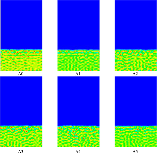
Figure 2. The effect of system pressure on membrane-forming morphology.
Download figure:
Standard image High-resolution imageEffect of system temperature on PVDF membrane
From the control equation of the model, it is obtained that the magnitude of the temperature T is related to the momentum equation in the control equation, so the magnitude of its value is closely related to the model. The specific setting values are shown in Table V. The temperature value T was taken as the only variable value, and the effect of cross-migration rate was ignored in the setting of the system because of the possible complex relationship between system pressure and cross-migration rate. The initial conditions of the two layers are shown in Table IV.
Table V. Setting values of temperature.
| Number | B0 | B1 | B2 | B3 | B4 | B5 |
|---|---|---|---|---|---|---|
| MSS | 2000 | 2000 | 2000 | 2000 | 2000 | 2000 |
| MPP | 2 | 2 | 2 | 2 | 2 | 2 |
| T | 0 | 20 | 40 | 60 | 80 | 100 |
The simulation time of t = 8.0 × 10⁻⁵s was selected for comparative analysis, as shown in Fig. 3. From the overall view of the figure, the membrane pores are all slowly changing from dispersed points to a continuous state, and the interface between the polymer solution layer and the solidification bath connection are all relatively flat, but the top layer of the polymer solution is all slightly fractured. With the increase of the system temperature, among them, Figs. B0 ∼ B3 show that the thickness of the inter-pore wall thickness after membrane formation decreases in turn, and the pore diameter after membrane formation increases in turn, and the trend in Figs. B3 ∼ B5 is similar to that of B0 ∼ B3, but the trend pattern of polymer volume fraction in Figs. B2 ∼ B3 is opposite to that of B0 ∼ B3, which indicates that the influence of the system temperature T value on the morphology of membrane formation has a certain peak, but its specific value needs to be further explored through experiments.
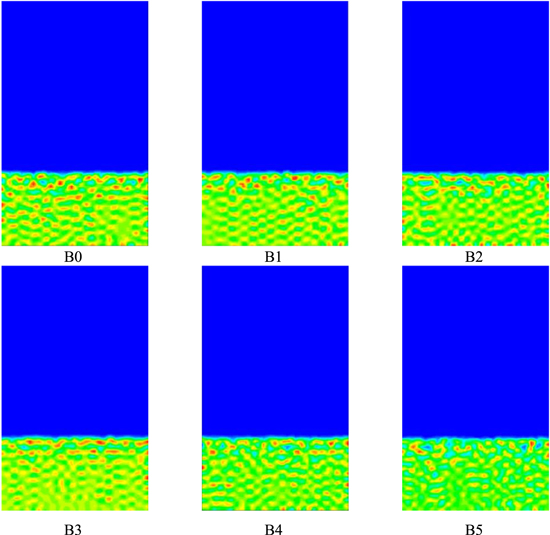
Figure 3. The effect of system temperature on membrane formation morphology.
Download figure:
Standard image High-resolution imageEffect of initial solvent concentration on PVDF membrane
The initial concentration (volume fraction) of the polymer was fixed and the initial volume fraction of solvent and non-solvent was varied to study the effect of the initial concentration of solvent on the membrane morphology. The volume fraction of polymer in the fixed polymer solution was 5%, and the percentage of DMAc and H2O were varied sequentially, and the specific ratios between them are shown in Table VI.
Table VI. Initial composition in polymer solutions.
| Series |
 p
p
|
 s
s
|
 ns
ns
|
|---|---|---|---|
| C1 | 0.05 | 0.05 | 0.90 |
| C2 | 0.05 | 0.10 | 0.85 |
| C3 | 0.05 | 0.15 | 0.80 |
| C4 | 0.05 | 0.20 | 0.75 |
| C5 | 0.05 | 0.25 | 0.70 |
| C6 | 0.05 | 0.30 | 0.75 |
The simulation time of t = 5.5 × 10⁻⁴s was selected for comparison and analysis, as shown in Fig. 4. It can be seen from the figure that the simulated variation diagrams of the solvent systems with different concentrations follow roughly the same course, and when the volume fraction of the solvent increases, the morphology does not actually change significantly, despite the different final equilibrium concentrations. At the same time, as the solvent system in the polymer solution increases, a small change occurs in the solidification bath that is no longer the volume fraction of the lowest polymer in the time step, i.e., completely blue. It indicates that the polymer in the polymer solution layer is diffusing into the solidification bath. The volume fraction of PVDF in the polymer layer in C4 is smaller compared to the other series. With the increase of solvent volume fraction in the system polymer solution layer, the volume fraction of polymer in the solidification baths of Figs. C1 ∼ C6 increased sequentially with a slight trend, where Figs. C1 ∼ C2 illustrated that the thickness of inter-pore wall thickness increased sequentially after membrane formation, while the pore diameter decreased sequentially after membrane formation, the trend in Figs. C2 ∼ C4 was opposite to that of C1 ∼ C2, and Figs. C5 ∼ C6 were similar to that of Figs. C2 ∼ T4, but Figs. C4 ∼ C5 were similar to that of C1 ∼ C2, indicating that the initial component of solvent in the system polymer solution had some influence on the morphology of membrane formation.
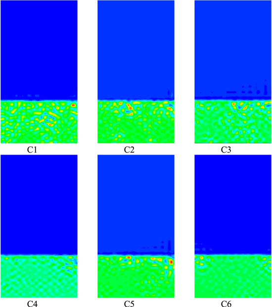
Figure 4. Effect of initial solvent composition in polymer solution on membrane morphology.
Download figure:
Standard image High-resolution imageSimulation of non-solvent water addition on PVDF membrane
The initial concentration (volume fraction) of the polymer was fixed and the initial volume fraction of solvent and non-solvent was varied to study the effect of the initial concentration of the solvent on the membrane morphology. The volume fraction of polymer in the fixed polymer solution was 25%, and the percentage of DMAc and H2O was varied sequentially, and the specific ratios between them are shown in Table VII.
Table VII. Initial composition in polymer solution.
| Series |
 p
p
|
 s
s
|
 ns
ns
|
|---|---|---|---|
| D1 | 0.25 | 0.75 | 0.00 |
| D2 | 0.25 | 0.73 | 0.02 |
| D3 | 0.25 | 0.71 | 0.04 |
| D4 | 0.25 | 0.69 | 0.06 |
| D5 | 0.25 | 0.67 | 0.08 |
| D6 | 0.25 | 0.65 | 0.10 |
A comparative analysis of the polymer solution simulation plots for different non-solvent systems is shown in Fig. 5. With the increase of non-solvent volume fraction in the system polymer solution layer, where Figs. D1 ∼ D2, D3 ∼ D4, D5 ∼ D6 illustrate that the thickness of the inter-pore wall thickness after membrane formation increases in order, while the pore diameter after membrane formation increases in order, and Figs. D2 ∼ D3, D4 ∼ D5 illustrate that the thickness of the inter-pore wall thickness after membrane formation decreases in order, while the pore diameter after membrane formation increases in order, indicating that the non-solvent initial component in the system polymer solution has a certain influence on the membrane formation morphology.
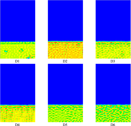
Figure 5. Effect of non-solvent initial components of polymer solutions on membrane morphology.
Download figure:
Standard image High-resolution imageEffect of initial polymer concentration fluctuations on PVDF membranes
In order to verify the validity of the model, experimental membranes were made for different polymer concentrations and used for comparison with the simulation result plots. To investigate the effect of polymer concentration on the morphological evolution of PVDF membranes, the H2O/DMAc/PVDF system was selected for experimental membrane production and numbered as group A membranes. Simulations were also carried out using different combinations of initial concentrations in polymer solutions and these combinations of initial concentrations, i.e. two layers of initial conditions, are shown in Table VIII. The  p
and
p
and  s
in the polymer solution were changed, while keeping
s
in the polymer solution were changed, while keeping  ns
constant. The set values of each parameter for the simulated process system are shown in Table IX.
ns
constant. The set values of each parameter for the simulated process system are shown in Table IX.
Table VIII. Table of composition of each component.
| Number | E1 | E2 | E3 | |
|---|---|---|---|---|
| Polymer solution layer |
 p
p
| 0.15 | 0.20 | 0.25 |
 s
s
| 0.80 | 0.75 | 0.70 | |
 ns
ns
| 0.05 | 0.05 | 0.05 | |
| Coagulation bath |
 p
= 0.01,
p
= 0.01, s
= 0.01,
s
= 0.01, ns
= 0.98
ns
= 0.98 | |||
Table IX. Setting values of system parameters.
| Number | MSS | MPP | MPL-NS (cm s−1) | MSS-NS (cm s−1) | ρ (g cm−3) | η(Pa°s) |
|---|---|---|---|---|---|---|
| E1 | 2000 | 2 | 16.8 × 10³ | 9.1 × 10³ | 1.0442 | 8.4 |
| E2 | 2000 | 2 | 16.85 × 10³ | 10.2 × 10³ | 1.088 | 8.65 |
| E3 | 2000 | 2 | 16.9 × 10³ | 10.9 × 10³ | 1.1313 | 8.98 |
Figure 6 shows the performance of the membranes prepared by PVDF casting solutions with different initial polymer concentrations. The order of the porosity size is: E2 > E1 > E3, and the order of the pure water flux size is: E1 > E2 > E3. Combining the porosity with the pure water flux, the performance of the membranes made by the E3 system is the worst among them. As the polymer concentration increases, the membrane pore size increases first and then decreases, and the pure water flux gradually decreases.
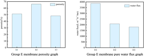
Figure 6. Performance diagram of E membrane.
Download figure:
Standard image High-resolution imageThe evolution of the membrane morphology (volume fraction of polymer ( p
) vs time) during the phase transition is shown in Fig. 7. Red indicates the maximum volume fraction of the polymer at each time step, blue indicates the minimum volume fraction of the polymer at each time step, and other colors fall in between.
p
) vs time) during the phase transition is shown in Fig. 7. Red indicates the maximum volume fraction of the polymer at each time step, blue indicates the minimum volume fraction of the polymer at each time step, and other colors fall in between.
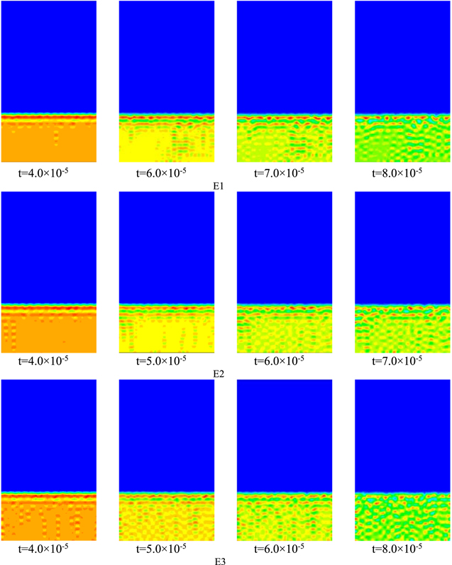
Figure 7. Effect of initial polymer concentration in polymer solution on membrane morphology.
Download figure:
Standard image High-resolution imageThe simulation starts with two layers of initial conditions, with the polymer solution (polymer and solvent) at the bottom at 30% and the solidification bath (non-solvent) at the top. The polymer stays almost completely in the polymer solution region, as shown in Fig. 7. The solidification bath is always blue in color (tiny polymer volume fraction). The phase separation process starts from the top of the polymer solution layer and proceeds downward in the laminar structure. 22 The final morphology of the PVDF membrane is an asymmetric structure 23 with a dense epidermal layer on top of the porous support layer, which is consistent with experimental observations.
With the increase of polymer volume fraction in the polymer solution layer, Figs. E1 ∼ E2 illustrate that the thickness of the inter-pore wall thickness after membrane formation increases sequentially, while the pore diameter after membrane formation decreases sequentially, while the trend in Figs. E2 ∼ E3 is opposite to E1 ∼ E2, indicating that there is a peak in the effect of polymer volume fraction in the polymer solution layer of the system on the morphology of membrane formation, from which it is indicated that the membrane performance formed by the E2 system is better.
Figure 8 shows SEM images of the membranes prepared with PVDF casting solutions with different initial concentrations of polymer, giving SEM images of the upper surface, lower surface and cross section. The lower surface appears almost smooth and more pores can be observed on the upper surface. The prepared PVDF membranes were all asymmetric, and the membrane thickness increased with increasing PVDF concentration, the macropore structure within the membrane was suppressed with increasing PVDF concentration, and the sponge-like structure size increased. PVDF At higher concentrations, the formed membrane has too much polymer at the interface with the solidification bath, forming a porous surface layer with lower porosity and a smaller water flux in the formed membrane. The validity of the model is verified by combining the experimental electron microscopy plots as well as the membrane properties, and the simulation result plots can be matched with the experiments.
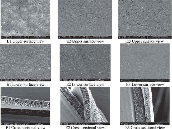
Figure 8. SEM photos of the membranes prepared by PVDF casting solution with different initial polymer concentrations.
Download figure:
Standard image High-resolution imageDiscussion
Analysis of the effect of system pressure and temperature on PVDF membrane
As shown in Fig. 2. As the system pressure increases, the polymer diffusion rate accelerates and the more blue fraction appears, i.e., the smaller the volume fraction of polymer in the grid in the time step. The schematic of each color can be seen in Fig. 1. And the blue part in the A5 chart is relatively reduced again. This indicates that the pressure value of the system can accelerate the phase separation rate and thus change the membrane formation structure, where the pressure value may slow down the phase separation rate relatively when it is too high. The obvious polymer lamellar structure layer can be seen in the A0 plot, the lamellar structure layer weakens in the A1 plot, and the lamellar structure layer gradually disappears in the A2 ∼ A5 plots, indicating that this lamellar structure is gradually broken with the increase of the pressure value. In the analysis of the simulated plot of the parameter of addition pressure compared with the previous parameters, the diffusion plot of the polymer tends to regularize the diffusion after its addition pressure.
The effect of system temperature on the membrane formation morphology can be seen in Fig. 3. As the temperature of the system T increases, the polymer diffusion rate accelerates and the degree of polymer dispersion gradually increases, and the blue part appears gradually, i.e., the smaller the volume fraction of polymer in the grid in the time step, and the schematic representation of each color can be seen in Fig. 1. The increase in temperature facilitates faster phase separation of the membrane, which in turn affects the membrane formation morphology.
Analysis of the effect of initial concentration of each component of polymer solution on PVDF membrane
With the increase of solvent in the polymer solution system, the polymer solution layer and the solidification bath connect the interface with a small fracture, but the undulation of its interface is small. This indicates that the top layer is destroyed during diffusion and that the concentration difference gradient is too large in diffusion and its diffusion drive breaks the energy setting at the interface. As the volume fraction of solvent in the polymer solution layer increases, the morphology changes from separated droplets to a bicontinuous mode. This also reduces the solvent gradient, which delays the onset of phase separation. The increase of the solvent system in the polymer solution leads to the increase of the interaction parameter between solvent and non-solvent, which leads to the increase of the mutual solubility zone in the phase diagram of the system, and then affects the membrane formation morphology.
From the overall view in Fig. 5, as the volume fraction of non-solvent in the polymer solution increases, the membrane pores gradually increase and the pore size also gradually increases, the morphology changes from separated droplets to a bicontinuous mode, and the interface between the polymer solution layer and the solidification bath connection is smoother. The non-solvent at low volume fractions moves downward in a laminar structure in the diffusion of the polymer, and breaks the laminar structure at higher volume fractions.
From the simulation results Fig. 7 as a whole, the membrane pores decrease but the pore size increases as the PVDF concentration increases. At the same time, the greater polymer volume fraction in the system is dispersed to a large extent, and the smaller polymer volume fraction is co-existed by droplets and continuums, implying the coexistence of finger-like pores and spongy pores in the system. At the same time, as the volume fraction of the polymer in the polymer solution layer increases, the effect on the bipartite line of the system gradually increases, affecting the interaction parameters between the components and, consequently, the membrane formation morphology. Meanwhile, this conclusion is fully verified in the experimental results in Fig. 8.
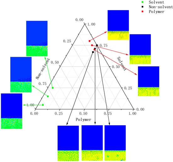
The initial moulding conditions of series C, D and E groups were described in the phase diagram by means of ternary phase diagrams, and then the effect of the concentration of each component on the formation process of PVDF membrane was compared and analyzed according to the graph of simulation results.
Figure 9 is a summary of the simulation results for each group of membranes according to the different variables, simulating the effect of different initial conditions in the polymer solution on the membrane formation morphology. The dots in the ternary diagram represent the initial conditions for the corresponding simulation results, where the green dots represent the different initial conditions for the simulated solvents in the Table IV series, the black dots represent the different initial conditions for the simulated non-solvents in the Table V series, and the red dots represent the simulation results with different initial polymer concentrations for comparison. The effect on the membrane formation process under different initial conditions is also well represented.
Figure 9. Effect of initial polymer components in polymer solution on the morphology of PVDF membrane.
Download figure:
Standard image High-resolution image
Conclusions
By simulating the effect of system pressure and temperature on the membrane formation process and by comparing the simulation plots of the effect of solvent, non-solvent, and initial polymer concentration fluctuations in the polymer solution layer on the phase separation process of PVDF membranes, it can be concluded that:
- (a)It can be seen based on the simulation results. With the addition of system pressure, the diffusion pattern of the polymer tends to regularize and the diffusion process of the polymer becomes more homogeneous. It makes the thickness of the formed membrane more uniform. It also improves the average pore size and porosity of the membrane to some extent.
- (b)As the temperature T of the system increases, the polymer diffusion rate is accelerated and the degree of polymer dispersion is gradually increased, which is conducive to accelerating the phase separation rate of the membrane and thus affecting the membrane-forming morphology.
- (c)From the point of view of the degree of influence of the concentration of each component in the polymer solution on the phase separation process of the membrane, the degree of influence of the starting concentration of each component in the polymer solution: polymer > non-solvent > solvent. The volume fraction of the polymer determines the morphology of the membrane, as it determines where the system enters the spinodal line and the ratio of the two phases.
Acknowledgments
The authors gratefully acknowledge the financial support from the Shaanxi Provincial Key R&D Project "Research and Application of Key Technologies for Conversion of Organic Waste into High-Quality Fertilizer" (Project No. 2021NY-188).
The authors would like to thank the School of Urban Planning and Municipal Engineering, Xi'an Polytechnic University for providing the experimental equipment. We would like to thank the supervisors from Xi'an Polytechnic University and OIL & GAS TECHNOLOGY RESEARCH INSTITUTE CHANGQING OILFIELD COMPANY for their guidance and insight into the direction of the research.