Abstract
A phenomenological model of the bulk force exerted by a lithium ion cell during various charge, discharge, and temperature operating conditions is developed. The measured and modeled force resembles the carbon expansion behavior associated with the phase changes during intercalation, as there are ranges of state of charge (SOC) with a gradual force increase and ranges of SOC with very small change in force. The model includes the influence of temperature on the observed force capturing the underlying thermal expansion phenomena. Moreover the model is capable of describing the changes in force during thermal transients, when internal battery heating due to high C-rates or rapid changes in the ambient temperature, which create a mismatch in the temperature of the cell and the holding fixture. It is finally shown that the bulk force model can be very useful for a more accurate and robust SOC estimation based on fusing information from voltage and force (or pressure) measurements.
Export citation and abstract BibTeX RIS

This is an open access article distributed under the terms of the Creative Commons Attribution Non-Commercial No Derivatives 4.0 License (CC BY-NC-ND, http://creativecommons.org/licenses/by-nc-nd/4.0/), which permits non-commercial reuse, distribution, and reproduction in any medium, provided the original work is not changed in any way and is properly cited. For permission for commercial reuse, please email: oa@electrochem.org.
Lithium intercalation and de-intercalation result in volumetric changes in both electrodes of a li-ion battery cell. At the anode, carbon particles can swell by as much as 12% during lithium intercalation, and the resulting stress can be large.6 Commercial battery packs involve numerous cells assembled to occupy a fixed space as shown in Fig. 1 and held in mild compression to resist changes in volume associated with lithium intercalation and de-intercalation. A small compression prevents de-lamination and associated deterioration of electronic conductivity of the electrodes. A large compression, however, can decrease the separator thickness and lead to degradation and power reduction due to the separator pore closing.18

Figure 1. Battery cells under compression in a Ford fusion HEV battery pack (left). The disassembled array after the compression bars have been removed making the unconstrained cells and spacers between them more visible in their expanded condition (right).
The effect of expansion and the system's mechanical response on the cell performance and life18,5,2,24 are under intense investigation with studies ranging from the micro-scale,4,6,24 the particle level,4 and multiple electrode layers.22,8 While progress toward predicting the multi-scale phenomena is accelerating,9,28 the full prediction of a cell expansion and its implications to cell performance depends heavily on the boundary conditions associated with the cell construction and electrode tabbing and crimping. Moreover, the wide range of conditions with respect to C-rates and temperatures that automotive battery cells must operate make the physics-based modeling approach very challenging.17 Finally, measuring and quantifying the internal stress or strain to tune or validate the multi-scale models requires complex instrumentation.23,30 In contrast to the micro-scale, the macro-scale stress and strain responses are directly observable and measured with high accuracy,16,19,26 thus could be used to develop phenomenological models inspired by the underlying physics.
To this end, a phenomenological model is developed in this paper in an attempt to mimic the evolution of bulk force/stress and to quantify the contributions of state of charge dependent intercalation and thermal expansion. A rudimentary version of this model was used for limiting the power drawn to avoid damaging forces and stresses on the cell in Ref. 12. The model developed herein will enable a power management scheme that is conscious of mechanical limits similarly to the electric (voltage) and thermal limits as in Refs. 13 and 15. In this paper the feasibility of using the developed model for State of Charge (SOC) estimation is also highlighted.
Experimental
The Fixture
Prismatic Lithium-Nickel-Manganese-Cobalt-Oxide (NMC) batteries encased in a hard aluminum shell were used in this study. Each cell has a nominal capacity of 5Ah and has outside dimensions of 120 × 85 × 12.7 mm. Inside the aluminum case is a horizontal flat-wound jelly roll that has 90 × 77.5 × 11.7 mm. In this orientation, with the tabs facing upwards as shown in Fig. 2, the bulk of the electrode expansion results in outward displacement of the sides of the aluminum case when unconstrained.16 The packaging of the jelly roll makes the electrode expand primarily perpendicular to the largest face of the battery due to the wound structure and gaps between the electrode and casing around the top and bottom. This observed cell expansion is, consequently, exerted against the end-plates when the battery pack is assembled as shown in Fig. 1. The space between the batteries is maintained via a plastic spacer with dimples to preserve the airflow channels and still provide a means for compressing the batteries.

Figure 2. X-ray tomographic slices of the battery show the internal structure. The left figure shows a slice along the x-y plane, the electrode geometry, and opposing tab geometry on the sides of the cell. The right figure shows a slice from the side (y-z plane), and highlights the wound prismatic jelly roll structure.
To study the force dynamics in a battery pack, a fixture as shown in Fig. 3 was designed and used in all experiments reported in this article. The fixture consists of three NMC batteries connected in series sandwiched between two 1-inch thick Garolite plates. The flat Garolite surfaces allow for parallel placement and compression of the batteries inside the fixture, and are bolted together using four bolts, one in each corner of the plate; each bolt is instrumented with an Omega LC8150-250-100 sensor to measure the bulk force. The sensor is a 350 ohm strain gauge type load cell with a 450 N full scale range and 2 N accuracy. This arrangement of the fixture preserves a constant compressive distance between the two end Garolite plates which replicates the conditions experienced by cells in the pack.
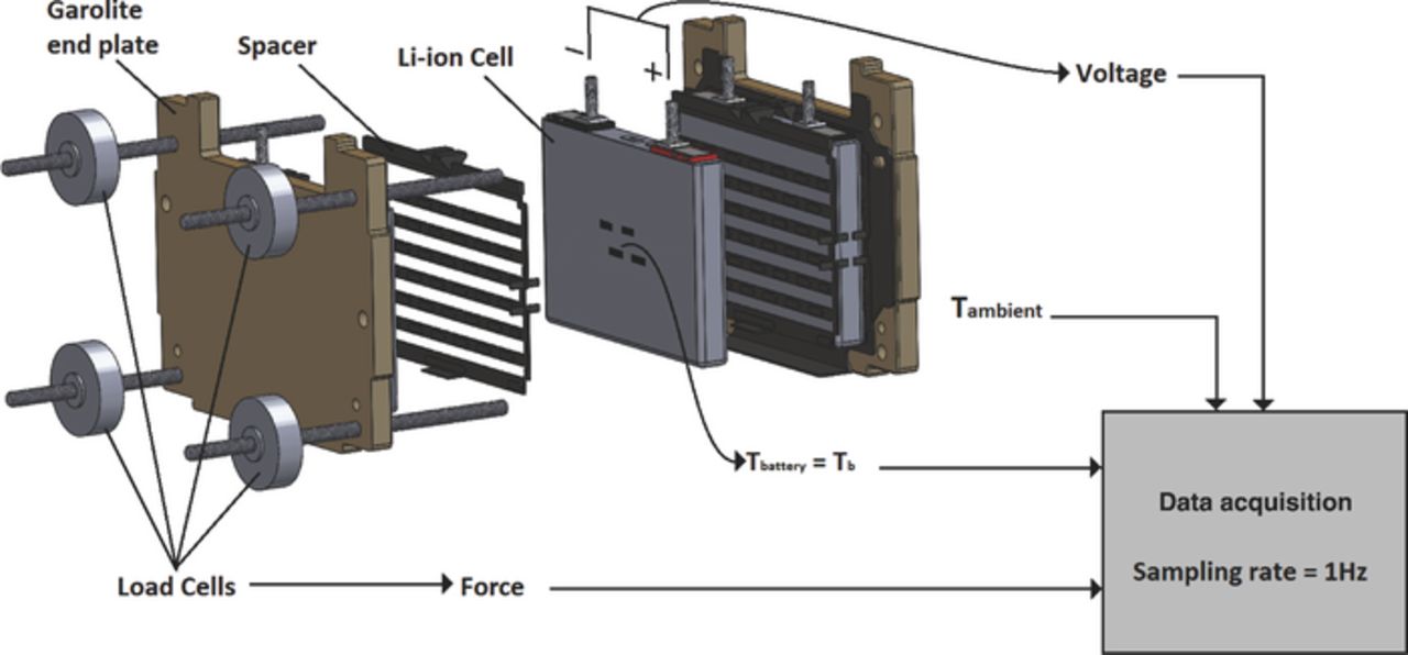
Figure 3. A schematic showing an expanded view of the fixture. Three cells are assembled between spacers and two Garolite end-plates to realistically imitate the mechanical conditions of the vehicle pack. External loading is applied to the batteries by tightening bolts and load cells are used to measure the bulk force associated with the cell expansion.
The fixture is placed in a Cincinnati Sub-Zero ZPHS16-3.5-SCT/AC environmental chamber to control the ambient/fixture temperature. Current excitation is provided by means of a Bitrode model FTV, and the resulting force and temperature data is acquired via a National Instruments NI SCXI-1520 strain gauge input module and 18-bit data acquisition card. The temperature, current, voltage and force data are sampled at a 1 Hz rate.
Observations based on bulk force measurements
Using the described fixture, and performing experiments (E1) and (E2) detailed in Appendix
Figure 4(a) presents the experimentally observed relation among Force, SOC and temperature, derived from the experiment (E1). At room temperature, the shape of the measured Force-SOC relation bears a striking similarity to the linear surface displacement of a similar unconstrained prismatic cell in Ref. 16 and interlayer spacing in the graphite anode.29 This observation can be explained by noting that in Li-ion cells with graphitic anodes, the volume expansion of the graphite is typically much larger than that of the cathode (Table I) and that the stress-intercalation state of the negative electrode exhibits a similar shape.21
Table I. Volumetric strain change of various compounds.27
| Electrode | Compound | Value [%] |
|---|---|---|
| Positive | LiCoO2 | +1.9 |
| LiNiO2 | −2.8 | |
| LiMn2O4 | −7.3 | |
| LiNi1/3Mn1/3Co1/3O2* | +2.44 | |
| Negative | Graphite C6 | + 12.8 |
*is the most similar to the positive electrode material in this study.

Figure 4. (a) Quasi-steady-state measurements of per-bolt force at various temperatures and SOCs. The curve at 25°C is represented at  . (b) Computed values of dF/dz and dV/dz for various SOCs and temperatures. The arrow attempts to track the position of the peak in the dF/dz curve as temperature changes. Notice that changes in ambient temperature tend to flatten the dF/dz curve.
In Ref. 3, the authors assert that the stress-SOC relation is to be expected to be independent of temperature and current. However, contrary to this claim, Fig. 4(a) shows a significant dependence of measured force on the temperature of the pack-fixture. Further, it can also be inferred that a change in temperature does not involve a simple linear superposition of the expected material expansion (contraction) due to temperature increase (decrease). This nonlinear effect can be seen by observing that for the same change in temperature, the increase in measured force at different SOCs is not the same. Figure 4(b) presents approximate curves of the rate change of measured force per-bolt with respect to change in SOC (dF/dz). From this figure, it is noted that as the temperature of the cell decreases, the dF/dz curve starts to get flatter and that the peaks in the curve constantly migrate to the left. This characteristic can perhaps be captured by a temperature dependent shift and scaling function.
Experimental data obtained from (E2) are plotted in Fig. 5 wherein the first two subplots are of primary interest. In this experiment, a 50 A, 1 Hz current was applied to the cell to effect a temperature increase in the cell through Joule heating; the gray section in subplot four indicates the period of pulse excitation. Notice that during this period, the temperature of the battery increases by ∼ 13 °C and the resulting per-bolt force is close to 400 N at 50% SOC. The value of force as the battery reaches thermal equilibrium is close to the force that is measured when the cell is fully charged (100% SOC) at 25 deg C. This observation further affirms our belief that thermal effects should not be ignored when modeling the bulk mechanical stress/ force in prismatic battery packs.

Figure 5. Test profile for the experiment that aims to study the influence of difference between fixture and battery temperature, Experiment (E2). Subplot one traces the trajectory of per-bolt measured force as time evolves; trajectories of ambient temperature Tamb and battery temperature Tb are plotted in subplot two; subplot three shows the evolution of SOC; and subplot four, the current applied. Note that the gray box in subplot four spans the duration of 1 Hz, 50A excitation.
Although, the exact physical origin of this nonlinear temperature effect is not understood, we will attempt in this paper to lump it to a temperature dependent effective Young's modulus. Hence we assume that the modulus of the cell changes with temperature and attempt to find a physical relationship that describes the shift and scaling that temperature variability imposes to the measured SOC-only dependent force  at one reference temperature.
A Phenomenological Model
It was experimentally observed that the measured quasi-static bulk force from a fixture that constrains prismatic cells is dependent on the temperature of the pack (here, the fixture and cells are assumed to be in thermal equilibrium). In this section, a simple physically motivated, yet phenomenological model is presented that aims to emulate the stress behavior of the fixture. The model to be presented consists of two parts – (a) a static component that accounts for SOC, z, by using the force measured at low C-rate at one temperature (battery and fixture soaked), hereafter called the reference temperature (Tref = 25°C); and temperature changes ΔTb and ΔTF of the battery Tb and the fixture TF from the reference temperature respectively; and (b) a dynamic component to capture the expected rate dependency of force.16 That is, the model can be expressed as
![Equation ([1])](https://content.cld.iop.org/journals/1945-7111/161/14/A2222/revision1/jes_161_14_A2222eqn1.jpg)
where Tb, TF and Tref are the battery, fixture temperature, and reference temperatures respectively and ΔT = [Tb − Tref, Tf − Tref]'; z(t) is the SOC of the cells in the pack;  and δf(t) is a dynamic additive term.
Steady state bulk force model
The fixture presented schematically in Fig. 3, is modeled equivalently as a bar in series with a spring as shown in Fig. 6; the bar and spring are representative of the lumped collective of cells and spacers in the fixture. In this equivalent mechanical model, the bar of length L is attached to a spring with spring constant ksp, and both are constrained and held in place by plates H apart (inner distance). The restorative force in the spring is the same as the sum of force measured by the load sensors and is computed by solving the force balance equation
![Equation ([2])](https://content.cld.iop.org/journals/1945-7111/161/14/A2222/revision1/jes_161_14_A2222eqn2.jpg)
where ΔL and ΔH are the changes in length of the bar and the fixture respectively. The stress σ is related to the force f by the surface area A of the battery which is under compression.

Figure 6. Approximate skeletal diagram of the fixture.
In deriving the mathematical relations in remainder of this section, the following assumptions pertaining to the thermal characteristics of the elements in the representative structure of Fig. 6 are made.
- It is a common observation that prismatic battery packs are held together with some minimal pre-stress. This initial pre-loading ensures that cells do not shift and also improve the conductivity of materials inside the cell. We assume that the pack which is being modeled is under some pre-stress.
- The bolts that hold the fixture together, much like the bar, are assumed to undergo thermal expansion. That is, suppose the temperature of the ambient changes by ΔTF ( = TF − Tref), then the bolts increase in length by ΔH. That is,where αF is the coefficient of thermal expansion.
![Equation ([3])](data:image/png;base64,iVBORw0KGgoAAAANSUhEUgAAAAEAAAABCAQAAAC1HAwCAAAAC0lEQVR42mNkYAAAAAYAAjCB0C8AAAAASUVORK5CYII=)
- The dependance of the Young's modulus of the bar on its temperature is assumed to be locally approximated by a quadratic function. That is,
- The length of the bar, aside from being impacted by the battery's temperature, is also affected by the SOC of the cell. The SOC dependent strain experienced by the bar is denoted as.
![Equation ([3])](https://content.cld.iop.org/journals/1945-7111/161/14/A2222/revision1/jes_161_14_A2222eqn3.jpg)


From the above assumptions, the change in length of the bar resulting from a ΔTb change in battery temperature and/ or SOC can be computed according to Eq. 4.
![Equation ([4])](https://content.cld.iop.org/journals/1945-7111/161/14/A2222/revision1/jes_161_14_A2222eqn5.jpg)
Suppose that, when the fixture and the cells in the pack are in thermal equilibrium with the ambient whose temperature is equal to Tref, the bulk force is measured over the entire rage of SOC. Denote by  , the function that relates SOC to measured force at T°refC. That is,
![Equation ([5])](https://content.cld.iop.org/journals/1945-7111/161/14/A2222/revision1/jes_161_14_A2222eqn6.jpg)
From the above, and by representing the longitudinal cross-sectional area of the cell by A, the restorative force in the spring at any temperature of fixture and battery can be computed as follows.
![Equation ([6])](https://content.cld.iop.org/journals/1945-7111/161/14/A2222/revision1/jes_161_14_A2222eqn7.jpg)
Substituting for  from Eqs. 5 into Eq. 6 and solving for f(ΔT, z) = σA, the measured force at any value of fixture and battery temperature, and at any SOC is expressed as
![Equation ([7])](https://content.cld.iop.org/journals/1945-7111/161/14/A2222/revision1/jes_161_14_A2222eqn8.jpg)
where ΔT = [ΔTb, ΔTF]'. Parameters of the static model in Eq. 7 are estimated using experimentally collected data using the methodology described Parameterizing the static model in Appendix
Table II. Estimates of various parameters in the static model that relates the temperature of the ambient and that of the battery, and the SOC of the battery, to the bulk force measured by load cells in the fixture depicted in Fig. 3.
| Parameter | Value | Unit | Comment |
|---|---|---|---|
| A | 1.02 × 10− 2 | m2 | measured |
| L | 4.5 × 10− 2 | m | measured |
| H | 6.0 × 10− 2 | m | measured |
| αF | 1.3 × 10− 5 | m/mK | assumed (steel) |
| αL | 3.44 × 10− 5 | m/mK | estimate |
| ksp | 1.73 × 10⁷ | N/m | estimate |
| k1 | 2.54 × 10⁸ | Pa | estimate |
| k2 | 1 × 10⁷ | Pa/°C | estimate |
| k3 | 1.44 × 10⁵ | Pa/°C2 | estimate |
The first three parameters in Table II correspond to physical dimensions which have been measured. The thermal expansion coefficient for steel is assumed for αF corresponding to the bolts. The estimated thermal expansion of the battery αL is reasonable for the given materials comparing to the values provided in Ref. 22. The estimated value for the spring constant ksp corresponds to the plastic separator, given the contact area and width of the separators this corresponds to an effective modulus of Esp = ksp*Lsp/Asp = 0.75 GPa, which is also reasonable for injection molded plastic.
Remark1. In the above derivation, the function  deserves special attention. The functional form of
  is empirically derived and is valid only for conditions identical to that when the function was initially parameterized. Particularly, if the pre-stress of the pack changes, be it owing to a change in the fixture or irreversible deformation of the batteries themselves, the function
  may not be valid as originally parameterized.
Dynamic bulk force model
In the previous subsection, a static model accounting for the influence of temperature (both ambient and fixture) and intercalation on the measured bulk force was modeled; however, the static model does not entirely capture the response of the actual system. As an example consider the measurements derived from experiment (E1); in particular, force measurements from the end of the Constant Current (CC) phase of every CCCV step (Step (S1.5) of experiment (E1) Parameterizing the static model in Appendix

Figure 7. (a) The relaxation in force at the end of the constant current phase of CCCV in Step (S1.5) in experiment (E1). Each individual curve is the difference between the measurement and the static model's output. (b) Comparing the relaxation in force following CC as in (a) at 25°C with different initial starting SOCs.
There are two principle observations to made by inspecting Fig. 7(a); the first observation is that the difference appears to exhibit some dynamics as the current is reduced to zero and during the ensuing relaxation period. One could contend that this observation is related to the internal temperature of the cell lagging behind the surface and undergoing some dynamics. Spatial distribution of temperature (along the thickness) inside the cell would result in a volume averaged expansion that is different from that computed using the parameters of the static model using the measured surface temperature, and could account for the difference presented in Fig. 7(a).
To test the above theory, the thermal model of the battery cell used in this study, presented in Ref. 1, was used to simulate the temperature in a prismatic cell soaked at different temperatures, in response to a 1C constant charge starting from ∼ 0% SOC. Fig. 8 presents the trajectory of the difference in temperature between the hottest and coolest spots in the battery as it was charged and allowed to rest, and Table III tabulates the max norm of the difference. The maximum difference in temperature is computed to not exceed 0.25°C, this difference is found to be unable to account for the difference in force presented in Fig. 7(a).
Table III. L∞ norm of the temperature differential and the change in static force prediction for this difference in temperature.
| Tamb (°C) |  (°C) (°C) | Δf (N) |
|---|---|---|
| −5 | 0.24 | 6.1 |
| 10 | 0.127 | 3.8 |
| 25 | 0.08 | 0.5 |

Figure 8. Trajectory of the temperature differential between the hottest and coolest spots of a cell along a 1C constant charging profile that is followed by rest; under different ambient conditions.
Figure 7(a) also provides reason to believe that the dynamics during relaxation is dependent on the temperature of the cell. As the cell's temperature increases, the effective error decreases while the time constant for the relaxation appears to not change noticeably.
To ascertain if the value of the difference between the measured and the static model's prediction is dependent on the initial SOC at which the charging operation (CCCV protocol) was initiated, Figure 7(b) traces two separate curves. The dashed curve shows the evolution of force for the case when the charging operation was initiated with the cell close to 5% SOC; the dash-dotted curve presents the case when the initial SOC was 50%. Since in both cases, the battery was charged at the same rate, 1 C, the time to reach the end of CC phase for the first case is almost twice that of the second. From Fig. 7(b), by comparing the values of the peaks of the curves, it is immediately apparent that the duration of charge appears to have an impact on the maximum value of the difference, suggesting that the state that affects bulk force, might have a rather large time constant.
Based on the above observations and inspired by the dynamics of dashpot, the dynamic equations of δf is written as
![Equation ([8])](https://content.cld.iop.org/journals/1945-7111/161/14/A2222/revision1/jes_161_14_A2222eqn9.jpg)
In a bid to reduce the model complexity and inspired by the current rate dependency of measured expansion results presented in Ref. 16, as a first attempt, we employ the following first order dynamic equation to describe the difference between the measured data and the static model.
![Equation ([9])](https://content.cld.iop.org/journals/1945-7111/161/14/A2222/revision1/jes_161_14_A2222eqn10.jpg)
where δf is the deviation from the static bulk force, I is the battery current; ζ1 and ζ2 are tunable parameters and assumed to be temperature dependent. These parameters are estimated by solving a least square optimization problem described in Appendix
Table IV. Parameters of the dynamic model.
| Temperature (°C) | |||
|---|---|---|---|
| Parameters | −5 | 10 | 25 |
| ζ1 | −0.0001 | −0.0001 | −0.0003 |
| ζ2 | 0.0197 | 0.0116 | 0.0083 |
Accuracy of the model
The final form of the bulk force model, with an aim of describing the influence of intercalation, temperature and current on the measured force, is expressed in terms of nominal force-SOC characteristic,  and a temperature dependent Young's modulus, E(Tb), as follows
![Equation ([10])](https://content.cld.iop.org/journals/1945-7111/161/14/A2222/revision1/jes_161_14_A2222eqn11.jpg)
where TF(t), Tb(t) are the trajectories of ambient and cell temperatures respectively; Q is the capacity of the cell in Ampere hours (Ah) and I is the battery current in Amperes; z is the state of charge (SOC).
Using parameter estimates computed Model parameterization in Appendix

Figure 9. Measured total force at various state of charges and temperatures compared with fit using the model, at steady state. Observe that as the temperature of the battery changes, the isothermal force curve translates vertically and also gets scaled.

Figure 10. The first subplot traces the trajectory of measured bulk force (black) and the outputs of the static (red) and full models (green), for the input profile shown in Fig. 12. The errors between measurement and model fit are plotted in the second subplot; note that the errors increase as operating temperature decreases. Root-mean-square error of the full model is 36.3% less than that when using the static model only.
In this section, a phenomenological dynamic model for the relation among bulk Force, SOC, Temperature and current was developed. The developed model uses measured data at a reference temperature (Tref), taken to equal 25 °C, to describe the evolution of force as the current, and battery and ambient temperature of the fixture change. The next section studies the simple case when temperature effects are not significant in using the developed model to check the feasibility of estimating the SOC of Li-ion cells, specifically for the chemistry used in this study.
Improving SOC Estimation with Bulk Force Measurements
Accurate information on the state of charge (SOC) of Li-ion cells is really important to ensure power availability, prevent under/over-voltage related damage and potentially to monitor battery degradation. The SOC of a Li-ion cell is a measure of the remaining energy in the cell. While there are a variety of definitions and expressions, in practice, it is considered to be the ratio of residual charge to total capacity in the cell. Since SOC is not measurable, it is commonly estimated from the terminal voltage by a process that is called inversion; in practice, this requires a model of the electrical dynamics.
The most widely used representative of the electrical dynamics is based on an equivalent circuit model including an open circuit voltage Voc in series with a resistance Rs and a R-C pair constituted by another resistance R and capacitance C. The representative dynamics of the equivalent circuit model used in HEVs is given by
![Equation ([11])](https://content.cld.iop.org/journals/1945-7111/161/14/A2222/revision1/jes_161_14_A2222eqn12.jpg)
where zk denotes SOC, vck represents the bulk polarization, Voc( · ) is the nonlinear relation between open circuit voltage and SOC (refer Fig. 11), Rs is the series resistance of the equivalent circuit model and V is the measured terminal voltage. Variables αz, αv and βv are related to the parameters of the equivalent circuit model through the following

where ts is the duration of the sampling period assumed in discretizing the continuous time dynamics of the OCV-R-RC model; Q is the capacity of the cell in Ah, R and C are the resistance and capacitance of the equivalent circuit model respectively.

Figure 11. Comparison of the rate change of Open Circuit Voltage (Voc) and intercalation related bulk force,  , with respect to State of Charge, z.
Recent papers such as25,20, concern themselves with novel architectures that invert the voltage dynamics. Unfortunately there are some SOC ranges in which these dynamic equations are not robustly invertible, making SOC estimation hard; i.e. small perturbations to the measured voltage can result in large changes to the estimates. This is particularly pronounced during normal operation of Hybrid Electric Vehicles (HEVs) which operate over a constrained SOC window, typically [0.3,0.7]. In this section, we investigate the feasibility of using force measurements and the developed model to improve the estimation of SOC over this interval, where conventional measurements are inadequate.
We assert that it is feasible to use force measurements and that doing so can improve the accuracy of estimates of SOC. To show this, we suppose that measurements of terminal voltage, cell current, bulk force, ambient and cell temperatures are available over N+1 successive discrete samples. Then by considering two cases, each with a different collection of measured data, we show that there is a SOC interval of interest where using bulk force measurements can improve estimates of SOC. These two cases are distinguishable based on the inclusion of force measurements. In the interest of simplifying the following arguments, in the remainder of this section, the influence of the dynamic term and temperature are omitted, although a similar analysis is possible in its presence.
By stacking measurements of terminal voltage and bulk force, two vectors Y1 and Y2 are defined as

In a similar way, two vectors H1 and H2 are generated by propagating the models over the same interval, [0, ..., N], respectively.

With the above setup, the SOC estimation problem for each case can be formulated as finding (z0, vc0) that minimizes the error between measurements and model outputs, ||Yj − Hj||2, j ∈ {1, 2}. This cost minimization problem can be solved using a nonlinear optimization technique called Newton's iteration.14 To update the estimate of the solution in this technique, it is necessary that the Jacobian matrix of Hj with respect to (x0, vc0) be of full rank during every iteration.
For simplicity of expressions, assume that the ambient temperature is 25°C and set the value of N to one; the following expressions are obtained.
![Equation ([12])](https://content.cld.iop.org/journals/1945-7111/161/14/A2222/revision1/jes_161_14_A2222eqn16.jpg)
![Equation ([13])](https://content.cld.iop.org/journals/1945-7111/161/14/A2222/revision1/jes_161_14_A2222eqn17.jpg)
Suppose the value of αv ≈ 1 (as is usually the case, refer1), if  , then the Jacobian matrix of Eq. 12 becomes ill-conditioned and the unique solution may not be robustly identified.
Figure 11 presents the derivative of Voc and  with respect to SOC over the typical operation of a HEV. The derivative of voltage and force were numerically computed by smoothing the measured data. Upon careful inspection, it is evident that between 40% and 50% SOC,
  is almost zero suggesting that the inverse of Jacobian matrix of Eq. 12 is not robustly computable: a small perturbation such as measurement noise of terminal voltage could lead to a large deviation of SOC estimate. Over the same interval however, the value of
  is non-zero suggesting that the condition number of the Jacobian matrix in Eq. 13 is potentially smaller than that of the Jacobian matrix in Eq. 12 and hence the estimate of (z0, vc0) using the former is more reliable.
Note that over the SOC interval [0.3,0.7], the second derivative of  and Voc with respect to SOC complement each other – in the sense that they are both seldom zero together. This means that over this range of SOC, the inclusion of auxiliary force measurements improves the estimates; this observation is more pronounced between 30 and 50% SOC.
A similar methodology has been described in patent11 to estimate the SOC and SOH of Li-ion cells. However, the model used therein is very simple and fails to account for the nonlinear relation between force/stress and SOC and temperature. To the author's best knowledge, the above section is the first discussion that provides a mathematical reason for why one might want to use force/stress measurements when estimating electrical model related states in Li-ion cells. In addition we are able to quantitatively suggest the range of SOC over which force measurements may improve estimates (interval [0.3,0.5]).
Conclusions
In this paper, a phenomenological model is developed to mimic the bulk force in a battery pack. The proposed model is driven by the fixture and battery temperatures, current, and state of charge. A one-state dynamic model is included to capture observed behavior during change and discharge. The benefit of applying the proposed model to SOC estimation is investigated. It is found that bulk force model can improve the robustness of SOC estimation within the typical SOC range for HEVs. This framework can also be used to identify SOH of a battery because the irreversible swelling related to battery degradation leads to a gradual increase in measured bulk force, and will be pursued as a part of a future work.
Acknowledgments
The information, data, or work presented herein was funded in part by the Advanced Research Projects Agency-Energy (ARPA-E), U.S. Department of Energy, under Award Number DE-AR0000269.
Disclaimer
The information, data, or work presented herein was funded in part by an agency of the United States Government. Neither the United States Government nor any agency thereof, nor any of their employees, makes any warranty, express or implied, or assumes any legal liability or responsibility for the accuracy, completeness, or usefulness of any information, apparatus, product, or process disclosed, or represents that its use would not infringe privately owned rights. Reference herein to any specific commercial product, process, or service by trade name, trademark, manufacturer, or otherwise does not necessarily constitute or imply its endorsement, recommendation, or favoring by the United States Government or any agency thereof. The views and opinions of authors expressed herein do not necessarily state or reflect those of the United States Government or any agency thereof.
: Appendix A
Appendix. Experiments
The aim of this paper is to study the influence of temperature and intercalation on the measured bulk mechanical stress. To that end, the battery pack is subject to the following experiment, henceforth referred to as (E1), involving changes in ambient temperature and SOC of the pack. Figure 12 depicts the profile of current and ambient temperature in (E1). At every temperature ∈ { − 5, 10, 25, 45}°C, the sequence of steps followed is listed below.
- (S1.1) The cell is first charged using a constant current, 1C-rate1 (5A) constant voltage (4.2 V) charging profile using a CCCV protocol, until the current reaches C/20 (0.25 A) at a fixed ambient temperature of 25°C as regulated by the thermal chamber. Follow charge by a three hour rest.
- (S1.2) Pulse discharge using 0.5C current pulse to reduce the SOC and rest for two hours.⋆
- (S1.3) Repeat (S1.2) until SOC reaches five percent.
- (S1.4) Rest for two hours.
- (S1.5) Charge to 100% using the CCCV protocol with 1C constant current and C/20 cutoff, and rest for three hours.
- (S1.6) Discharge at 0.5C-rate until SOC reaches 50% and rest for two hours
- (S1.7) Set ambient temperature to 25°C.▲
- (S1.8) Charge to 100% using 1C current and rest for three hours.
- (S1.9) Discharge to 50% SOC using 0.5C current.
- (S1.10) Rest for two hours and repeat (S1.1) at a new temperature.

Figure 12. Test profiles of current, SOC, and temperature for parameterization of bulk force response.
Notes 1.
- ⋆The State of Charge (SOC) of the cell is computed by coulomb counting. The pulses applied, as the pack is discharged until 5% SOC, are not identical. The SOCs at the end of the various pulses are, in order of occurrenceThis discharge profile, pulsing and resting, is the same at every temperature.
- ▲As a protocol, we have chosen to change the temperature of the pack only at 50% SOC. In addition, before every change in ambient temperature, an intermediary step wherein the ambient is raised/ lowered to 25°C is performed. This decision is motivated by a need to ensure that the prestress in the pack and or the sensors does not drift; changing prestress influences the dynamics and drifting sensors render the experimental data unreliable. Further, this step could also reduce the impact of any path dependence of measured force on the trajectory of temperature and SOC.
- ▼Note that in the designed experiment, each change in temperature and SOC is followed by a relaxation period to allow for equilibration of terminal voltage, cell temperature and force measurements. Steps (S1.8) and (S1.9) are performed to reduce any ambient temperature dependent stress accumulation.

Based on measurements derived from the experiment (EI) described above, we create two different data-sets:
- (E1.1) A quasi-steady-state map of the force measured at various SOCs and at various temperatures (Steps (S1.2) and (S1.3)).
- (E1.2) Transient data in which the measured force undergoes some dynamics, either owing to a change in SOC or temperature.
Experiment 2 (E2)
The second experiment performed on the fixture, attempts to isolate the influence of a persistent temperature differential between the ambient and the battery on the measurements of bulk force. To create this difference in temperature, the fixture is allowed to soak at room temperature inside a temperature controlled chamber until measurements of force and temperature reach equilibrium. Thereafter, the test profile can be broken into the following
- (S2.1) The pack is charged until the SOC reaches 100% using a CCCV protocol – the constant current employed is at 1C and the discharge cutoff is C/20 A.
- (S2.2) Following a rest of 1.5 hrs, the pack is discharged using a 1C current until the pack's SOC reaches 50%.
- (S2.3) Upon resting for a further 1.5 hours, the cell is excited with bi-directional rectangular pulse current for a duration of 2.5 hours. The amplitude of the current is 50 A and its frequency is 1 Hz.
Figure 5 depicts the trajectory of total force, temperatures and SOC that are a consequence of applying the above steps pertaining to experiment (E2).
: Appendix B
Appendix. Model parameterization
Parameterizing the static model
This section describes the approach adopted in parameterizing the model. the parameters of that we seek to estimate can br expressed as Λ = [αL, ksp, k1, k2, k3]'.
The force at any SOC and any value of fixture and battery temperature was derived in Eq. 7 and is reproduced, for convenience, below.

For convenience, let the modulus (Eb) in the above static model can be re-written as
![Equation ([B-1])](https://content.cld.iop.org/journals/1945-7111/161/14/A2222/revision1/jes_161_14_A2222eqn20.jpg)
![Equation ([B-2])](https://content.cld.iop.org/journals/1945-7111/161/14/A2222/revision1/jes_161_14_A2222eqn21.jpg)
By substituting the expression for temperature dependent modulus E(Tb), and by defining the following terms,
![Equation ([B-3])](https://content.cld.iop.org/journals/1945-7111/161/14/A2222/revision1/jes_161_14_A2222eqn22.jpg)
the bulk force is expressed as
![Equation ([B-4])](https://content.cld.iop.org/journals/1945-7111/161/14/A2222/revision1/jes_161_14_A2222eqn23.jpg)
Using the above equation, model parameterization is performed in two stages. In the first stage, the values of γi are estimated using data from experiment (E1.1); these estimates are in-turn used in the second phase to identify the individual parameters in Λ by utilizing the fact that αF corresponds to the thermal expansion coefficient of steel. In the ensuing discussion, the following notations are adopted — vectors are denoted using capitalized variables (X); individual elements of vectors are denoted using small letters and are indexed in their subscript (xi); and matrices are denoted in block capitals (A).
The four unknowns in Eq. B-4 do not all appear linearly and hence a nonlinear optimization problem is to be solved to estimate their values. Using data-set (E1.1), we solve the following global optimization problem to arrive at estimates of γ1, ..., 4
![Equation ([B-5])](https://content.cld.iop.org/journals/1945-7111/161/14/A2222/revision1/jes_161_14_A2222eqn24.jpg)
where the measured force data, stacked into a vector, is denoted by Y; Z is the vector of SOCs, ΔT is a vector of battery temperatures along the trajectory, stacked; and g( · ) is as defined in Eq. B-4. The constraint in Eq. B-5 is motivated by physics that the modulus of the material be positive. The estimation is performed by repeated application of Genetic Algorithm (GA) and by refining the solution of GA using a local nonlinear optimizer based on Sequential Quadratic Programming (SQP).7
The second phase of the parameterization procedure is aimed at distinguishing between the values of the two terms that constitute γ1; specifically, to identify θ1 and θ2. This is performed by minimizing the Least Squares minimization of Eq. B-6 using the data collected in experiment (E2).
![Equation ([B-6])](https://content.cld.iop.org/journals/1945-7111/161/14/A2222/revision1/jes_161_14_A2222eqn25.jpg)
where Θ = [θ1, θ2]'. The measurements of force along the trajectory are stacked into a vector F, as are the deviations of fixture and battery temperatures about the reference Tref, which are themselves denoted by ΔTF and ΔTb.
![Equation ([B-7])](https://content.cld.iop.org/journals/1945-7111/161/14/A2222/revision1/jes_161_14_A2222eqn26.jpg)
Using the solution to the problem in Eq. B-6 and relations in Eqs. B-3, the individual values of the parameters in the model are computed; these values are tabulated in Table II.
Computing variances of parameter estimates
For a general model of the form
![Equation ([B-8])](https://content.cld.iop.org/journals/1945-7111/161/14/A2222/revision1/jes_161_14_A2222eqn27.jpg)
where ε is an additive noise assumed to be Normally distributed, the estimate of error variance is given by
![Equation ([B-9])](https://content.cld.iop.org/journals/1945-7111/161/14/A2222/revision1/jes_161_14_A2222eqn28.jpg)
The Cramer-Rao bound of the least estimator is given by
![Equation ([B-10])](https://content.cld.iop.org/journals/1945-7111/161/14/A2222/revision1/jes_161_14_A2222eqn29.jpg)
The variance of θi in Θ, assuming the estimator is unbiased, is then the ai, i entry of the CRB matrix.
For the model under study, using the identified parameters, the CRB matrix is computed to equal

Then the variances of γ1, γ2, γ3 and γ4 are given by 5.56 · 10− 1, 1.65 · 10− 6, 1.07 · 10− 9 and 6.58 · 10− 3 respectively.
Remark 2. There are interesting observations to be made concerning the problem of estimating Λ using data collected in experiments (E1) and (E2). Using information from experiment (E1.1), none of the parameters in Λ can be individually identified; instead, variables γ1, ..., 4, combinations of parameters in Λ are estimated; γ1, ..., 4 are random variables with a mean and variance as computed above. Using γ1, ..., 4 to estimate θ1 and θ2 from the problem in Eq. B-6 is plagued by a potential issue — the variables C and d in Eq. B-6 are random variables (them being functions of random variables γ1, ..., 4). While it is desirable that a generalized least squares technique such as Total Least Squares (TLS)10 be applied, the fact that computing the variance of C is a nontrivial problem, has driven us to employ the Normal Least Squares (NLS) method in this paper. Having employed NLS, variances of parameters Λ, do not convey any meaningful information on the uncertainty in estimates and have been omitted.
Parameterizing the Dynamic Model
The dynamic model of δf is, for convenience, re-stated below.
![Equation ([B-11])](https://content.cld.iop.org/journals/1945-7111/161/14/A2222/revision1/jes_161_14_A2222eqn31.jpg)
where δf is the deviation from the static bulk force, I is the battery current; ζ1 and ζ2 are tunable parameters and assumed to be temperature dependent.
Parameters of the dynamic model, ϑ = [ζ1, ζ2]', are identified by minimizing the Euclidean norm of the difference between measurement and model prediction, the resulting parameters are ϑ*. That is, we solve the following optimization problem

where Nf is the number of measurement points, ts is the duration of the sampling period and zi is the SOC at the  data point. The first and the second equality constraints denote the dynamics and initial condition, respectively. In particular, the first equality constraint is constructed by applying the forward Euler to Eq. B-11. The model is trained using data-set (E1.2) at various ambient temperatures. The minimization problem is solved by using Sequential Quadratic Programming (SQP) and the identified parameters are provided in Table IV.
Footnotes
- 1
1C is the maximum magnitude of current that completely charges/discharges a cell in one hour uniformly in initial SOC.