Abstract
Battery performance is strongly correlated with electrode microstructural properties. Of the relevant properties, the tortuosity factor of the electrolyte transport paths through microstructure pores is important as it limits battery maximum charge/discharge rate, particularly for energy-dense thick electrodes. Tortuosity factor however, is difficult to precisely measure, and thus its estimation has been debated frequently in the literature. Herein, three independent approaches have been applied to quantify the tortuosity factor of lithium-ion battery electrodes. The first approach is a microstructure model based on three-dimensional geometries from X-ray computed tomography (CT) and stochastic reconstructions enhanced with computationally generated carbon/binder domain (CBD), as CT is often unable to resolve the CBD. The second approach uses a macro-homogeneous model to fit electrochemical data at several rates, providing a separate estimation of the tortuosity factor. The third approach experimentally measures tortuosity factor via symmetric cells employing a blocking electrolyte. Comparisons have been made across the three approaches for 14 graphite and nickel-manganese-cobalt oxide electrodes. Analysis suggests that if the tortuosity factor were characterized based on the active material skeleton only, the actual tortuosities would be 1.35–1.81 times higher for calendered electrodes. Correlations are provided for varying porosity, CBD phase interfacial arrangement and solid particle morphology.
Export citation and abstract BibTeX RIS

This is an open access article distributed under the terms of the Creative Commons Attribution Non-Commercial No Derivatives 4.0 License (CC BY-NC-ND, http://creativecommons.org/licenses/by-nc-nd/4.0/), which permits non-commercial reuse, distribution, and reproduction in any medium, provided the original work is not changed in any way and is properly cited. For permission for commercial reuse, please email: oa@electrochem.org.
Lithium-ion battery (LIB) electrodes have complex porous microstructures, which are linked to the macroscopic performance of these devices. Figure 1a shows a focused ion beam (FIB) cross section of a nickel-manganese-cobalt (NMC532) composite electrode imaged by scanning electron microscopy (SEM). In addition to the electrochemical active material, the electrode contains non-intercalating carbon and binder additives to promote electronic conductivity and mechanical integrity. Herein, the carbon/binder mixture is lumped as a single phase and referred to throughout this article as the carbon/binder domain (CBD). This simplification has been well-established in the LIB literature.1–6 With disparate CBD and active material particle sizes and morphologies, the resulting electrode contains a complex network of pores ranging from nanometer to micrometer length scales. Electrode battery macro-homogeneous electrochemical models often use porous electrode theory and thus abstract microstructural heterogeneity of composite electrodes using effective macroscopic properties.7–14 In porous electrode theory,11,15–18 electrodes are treated as homogeneous media with superimposed solid (active material) and electrolyte phases while inert phases are neglected (only their impact on the volume fractions is considered). Homogenization of the heterogenous microstructure medium through the use of effective parameters hinders the predictive capability of macro-homogenous models, where particle size distributions and morphological variations are ignored.
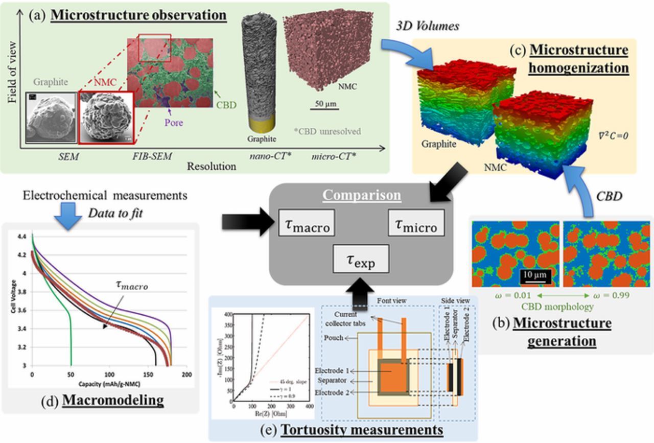
Figure 1. (a) Imaging of graphite/NMC532 powders and electrodes. (b) Adding a CBD phase with prescribed morphology, ω. (c-e) Electrode tortuosity τ, determined by three independent methods: (c) homogenization calculation on three-dimensional geometry where colors represent relative Li+ concentration, (d) fitting of macro-homogeneous model to rate data, (e) measurement using blocking electrolyte on symmetric cell.
One such example of effective parameters is the description of ionic transport in the electrolyte phase. Fast ion transport is necessary for the battery to sustain continuous high-rate discharge or charge currents, important, for example, for the fast charging of electric vehicle batteries.19–22 Ionic transport is described through multiple parameters in macroscopic models, one of them being the tortuosity factor, whose definition is given in the next paragraph. Applications requiring high energy density aim to maximize the electrode thickness (to increase the energy and reduce cost).23 However, experimental studies have shown that thick electrodes detrimentally affect the electrochemical performances and long-term cycling.24,25 Numerical modeling performed at high-rates have confirmed the electrochemical reaction is limited by the transport of lithium ions within the electrolyte, resulting in a severely reduced capacity for thick electrodes.23 Furthermore, Ebner et al.26 have shown for electrodes that share similar porosity, a lower tortuosity factor allows a significant increase in the C-rate (thus reducing the charging time). These results are a strong incentive to determine precisely the tortuosity factor.
Tortuosity, initially introduced by Kozeny27 and then developed by Carman,28 denotes the effect of the convoluted, tortuous path of the pores that hinder the Li-ion transport in the electrolyte phase. Several metrics of tortuosity are found in the literature.29–38 Each relates an effective transport property such as diffusivity, Deff, with the bulk intrinsic property, D0. In this work we consider the tortuosity factor36–38 noted τ and defined by Eq. 1, with ε the porosity. The tortuosity factor should not be confused with the tortuosity (defined elsewhere as the ratio of an effective path length to the domain's length33). For the microstructures considered in this study, pore connectivity was extremely high (isolated pores represent less than 1% of the total pore domain) and percolation was isotropic, so irrespective of whether total porosity or percolating porosity values are used, the calculated values of tortuosity factor would not be significantly affected. Tortuosity factor is sometimes replaced in the literature with the Bruggeman exponent29–33 p (cf. Eq. 2) or the MacMullin number34 NM (cf. Eq. 1), also called the formation factor.35 The same equations can be used to relate effective ionic conductivity Keff with the ionic conductivity of the bulk K0. Bruggeman theory31,32 provides a theoretical relation between porosity and geometric tortuosity for ideal geometries, where p is the Bruggeman exponent. For an ideal electrode packed with identically sized non-overlapping spheres p = 1.5; for pillars aligned in the transport direction p = 2.033. Note that these values correspond to particular cases of the empirical Archie's law (cf. Eq. 3).32 Their validity corresponds to cases where the insulating phase is present in a low volume fraction (i.e., high porosity) and represented by randomly distributed spherical (i.e., isotropic) mono-size particles for p = 1.5. Its application for actual electrode battery microstructures is a considerable simplification and thus should be considered with caution.33 In practical electrodes, higher Bruggeman exponents are commonly reported.12,39–41 Further, while Bruggeman theory implies that tortuosity factor can be related to porosity as τ = ε1 − p, in practice the tortuosity factor-porosity relationship is often described with a generalized form of the empirical Archie's law using a pre-exponential factor noted γ34,39,42 (cf. Eq. 3). This additional parameter γ allows the Bruggeman relationship to be scaled for different constituents and particle morphologies of the active material. At least two experiments − at different porosity − are required to determine the two parameters γ and α of this modified law.39 In either case, Bruggeman and Archie's Laws are only valid for the specific microstructure morphology for which their empirical parameters are fit, limiting their extensibility.33,35
![Equation ([1])](https://content.cld.iop.org/journals/1945-7111/165/14/A3403/revision1/d0001.gif)
![Equation ([2])](https://content.cld.iop.org/journals/1945-7111/165/14/A3403/revision1/d0002.gif)
![Equation ([3])](https://content.cld.iop.org/journals/1945-7111/165/14/A3403/revision1/d0003.gif)
As a consequence, many other tortuosity factor-porosity relationships have been derived in the literature.43–45 It is notable that several tortuosity factor-porosity relationships tend to agree in the porosity range of 0.4–0.7, while being significantly different for the lower values (due to different underlying assumptions), questioning the validity range of these expressions.33 Other microstructure parameters, for instance particle shape and orientation,26,46–48 geometric path length (also called the geometric tortuosity) and variation of the pore section area (factor of constriction)35,49 have been defined in the literature to provide a better understanding of the tortuosity factor. The purpose of these additional parameters is to discriminate the different contributions of the microstructure morphology on the effective diffusion, rather than to encompasses all of them in a unique parameter (the tortuosity factor or the Bruggeman exponent). For instance, Holzer et al.35 have proposed a geometrical determination of the tortuosity factor. For high porosity electrode materials, these other contributions are generally overshadowed by the porosity in the tortuosity-factor calculation. However, as the porosity decreases (e.g., energy-dense Li-ion battery electrodes) their weight may become more important and not taking them into consideration may then result in incorrect tortuosity factor predictions. This explains in part the poor predictive capability of tortuosity factor-porosity relationships for low porosity materials for which the literature reports a wide range of values26,33,34).
Given the three-dimensional microstructure geometry of an electrode, it is in theory possible to simulate the effective diffusivity of the microstructure and thus compute the tortuosity factor. This microstructure homogenization approach is enabled by the availability of microstructural geometry data from computed tomography (CT);14,50–55 although this approach does have limitations. These include (i) insufficient resolution to capture fine features, (ii) limited field of view (FOV) to capture a large enough volume to provide statistically relevant results, and (iii) insufficient image contrast to separate CBD from pore phase. With careful instrument selection and sample preparation, limitations (i) and (ii) can generally be addressed. Insufficient phase contrast (iii) remains an issue however, and CT images must currently be supplemented with focused ion beam scanning electron microscopy (FIB-SEM) to map CBD-phase geometry.50,56–59 FIB-SEM, however, rarely achieves a large enough representative volume size in a reasonable amount of time and this disparity in length scales between the two makes this approach somewhat questionable. Alternatively, some authors numerically generate the electrode active material microstructure60–64 and even the CBD65,66 through various numerical algorithms. However, given the algorithmic nature of these approaches, a generated CBD phase is not necessarily realistic. To circumvent these imaging limitations, this work uses a physics-based CBD phase description recently proposed by Mistry et al.,6 which accounts for necessary evaporation dynamics that govern the interfacial arrangement of the CBD phase to generate a plausible CBD geometry within the pore domain. The method reasonably predicts effective properties as well as performance trends.
A primary goal of this paper is to validate a microstructure model-based method for tortuosity prediction that can provide guidance for future designs of energy-dense, fast-charge capable LIB electrodes. Here, the tortuosity factor is calculated on multiple numerically generated microstructures with and without the generated CBD to evaluate the impact of this often neglected inert phase. A corrective factor (which is analogous to the CBD nanopore tortuosity factor, under assumptions discussed in Accounting for the CBD phase on the pore tortuosity section) is then derived to retrieve the correct tortuosity from the value calculated without the CBD. The corrective factor is evaluated for various microstructures with significantly different geometries and for different CBD nanopore networks. Furthermore, CT images are used to adequately resolve the active material phase with a large enough volume to give a representative volume. The tortuosity factor calculated on those images (for which the CBD is unresolved) is then adjusted using this corrective parameter. To assess the accuracy of the microstructure homogenization method enhanced with virtual CBD, this work compares model-predicted tortuosity factors to those obtained from direct measurement on symmetric cells infiltrated with a blocking electrolyte34,67 as well as to a macro-homogeneous model where tortuosity is fitted to electrochemical discharge experiments (cf. Fig. 1). The methodology aims to resolve the discrepancy in tortuosity estimation reported in the literature where results differ depending upon the chosen measurement, imaging, and/or numerical approach, as well as on assumptions on the CBD phase. Here, the modeling and experimental methods are applied to a library of graphite and NMC532 LIB electrodes with various loadings, porosities and thicknesses. Sources of numerical and experimental error are discussed as they relate to the ability to predict tortuosity factor.
Experimental Approach
Electrode library
A variety of Li-ion cathode and anode electrodes were fabricated by the Cell Analysis, Modeling and Prototyping (CAMP) facility at Argonne National Laboratory with four loadings ranging from 2.05 to 8.27 mAh.cm−2 and with porosities and thickness ranging from 34% to 52% and 34 to 205 μm, respectively. Cathode and anode active materials are Li(Ni0.5Mn0.3Co0.2)O2 (NMC532, TODA America Inc.) and CGP-A12 graphite (ConocoPhillips Inc.), respectively. Cathodes are fabricated using 90 wt% NMC532, 5 wt% C45 carbon (Timcal), and 5 wt% polyvinylidene fluoride (PVDF) (Solvay, Solef 5130) casted on a 20-μm-thick battery-grade aluminum foil. Anodes are composed of 91.8 wt% graphite, 2 wt% C45 carbon (Timcal), 6 wt% PVDF binder (KF-9300 Kureha) and 0.17 wt% oxalic acid casted on a 10-μm-thick battery-grade copper foil. Prior to casting on the metal foil support, components of each electrode are well mixed in a slurry using N-methyl-2-pyrrolidone (NMP) as solvent. To generate electrodes with varying porosity, tortuosity and thickness parameters, a cathode and anode coatings were tested in uncalendered (UNCAL) and calendered (CAL) states, for a total of 14 electrodes (7 cathodes and 7 anodes). The steel drum in the calendering machine set the desired thickness without tracking force. A complete list of electrodes with relevant parameters is presented in Table I.
Table I. Nominal properties of electrodes studied.
| Coating thickness | Volume fractionb | Density [mg.cm−2] | Loading [mAh.cm−2] | Experimental C-ratec | ||||||
|---|---|---|---|---|---|---|---|---|---|---|
| Material | Calendering | Designation | [μm]a | Pore | Active material | CBD | Coating | Active material | Active material | [mAh.gactive−1] |
| NMC | No | 1-UNCAL | 160 | 49.1 | 39.7 | 11.2 | 33.09 | 29.78 | 8.27 | 179 |
| Yes | 1-CAL | 129 | 36.8 | 49.3 | 13.9 | 178 | ||||
| No | 2-UNCAL | 140 | 51.8 | 37.6 | 10.6 | 27.39 | 24.65 | 6.84 | 179 | |
| Yes | 2-CAL | 108 | 37.5 | 48.8 | 13.7 | 180 | ||||
| No | 3-UNCAL | 106 | 47.4 | 41.0 | 11.6 | 22.60 | 20.40 | 5.66 | 183 | |
| Yes | 3-CAL | 88 | 36.6 | 49.5 | 13.9 | 182 | ||||
| Yes | 4-CAL | 34 | 33.5 | 51.9 | 14.6 | 9.17 | 8.25 | 2.29 | 178 | |
| Graphite | No | 5-UNCAL | 205 | 50.7 | 44.6 | 4.7 | 21.89 | 20.1 | 7.48 | 336 |
| Yes | 5-CAL | 165 | 38.8 | 55.4 | 5.8 | 300 | ||||
| No | 6-UNCAL | 173 | 51.8 | 43.6 | 4.6 | 18.08 | 16.6 | 6.17 | 330 | |
| Yes | 6-CAL | 131 | 36.3 | 57.7 | 6.0 | 282 | ||||
| No | 7-UNCAL | 140 | 51.4 | 44.0 | 4.6 | 14.70 | 13.5 | 5.02 | 351 | |
| Yes | 7-CAL | 110 | 38.0 | 56.1 | 5.9 | 351 | ||||
| Yes | 8-CAL | 44 | 38.4 | 55.8 | 5.8 | 5.88 | 5.51 | 2.05 | 363 | |
aMeasured with a micrometer. bObtained from recipe calculation. cExperimental C-rate (current that takes 1 hour to discharge the cell) determined from sequential increase in current.
Electrochemical characterization
For electrochemical measurements, half-cells consisting of lithium foil anode (purity = 99.9%, MTI Corp.), 40 μL of 1.2 M LiPF6 in ethyl carbonate/ethyl methyl carbonate (EC:EMC, 3:7 w/w, Tomiyama, Japan) held in a Celgard 2325 (PP/PE/PP) separator, and a 14.2-mm-diameter working electrode (NMC532 or graphite) were assembled in a standard 2032-type coin cell. Prior to assembling coin cells within the glove box, all electrodes and separators were dried at 120°C and 70°C, respectively, in a vacuum oven, also housed in the glove box. All cells were placed in a temperature-controlled chamber at 30°C to minimize artifacts arising from temperature fluctuations. Electrochemical discharges at current rates of 0.2C, 0.5C, and 1C for the NMC and charges of 0.5C for the graphite were performed using a MACCOR industrial battery cycler in a specified voltage window. The data processed in this manuscript were collected after three conditioning cycles at 0.1C.
Tortuosity direct measurement
Each tortuosity measurement was done by collecting AC impedance or electrochemical impedance spectroscopy data for a symmetric cell infiltrated with a non-intercalating or blocking electrolyte, according to a method described by Landesfeind et al.34 20 mM tetrabutylammonium hexafluorophosphate (TBAPF6) in a 1:1 (w:w) mixture of ethylene carbonate (EC) and dimethyl carbonate was used as the blocking electrolyte. All salts and solvents were obtained from Sigma Aldrich. To make the symmetric cell for this test, a stack of a smaller-area electrode and a separator (Celgard 3501) and a larger-area electrode were placed in a pouch cell, according to the configuration shown in Fig. 1e, and sealed using an electrical heat sealer. The smaller-area electrode was cut to 4 cm2 and the larger-area electrode was cut slightly larger than the first electrode to make exact alignment of the two electrodes less critical. After allowing the cell to sit for approximately 24 hours to ensure proper wetting of the sample, the pouch cell was then tested using a Bio-Logic SP-200 potentiostat. Electrochemical impedance spectroscopy measurements were taken with a 10-mV perturbation and no DC voltage bias (open circuit voltage of symmetric cells is essentially zero) for an appropriate frequency range. The cell was run under an external pressure of approximately 45 kPa, produced by placing a rubber layer and a metal weight on top of the pouch cell. The resulting Nyquist spectrum was then fitted to a transmission line model34 to obtain effective ionic conductivity of each porous electrode film. This can be directly translated to a McMullin number or, knowing the porosity of the sample, to a tortuosity (cf. Eq. 1). Each sample was tested twice to check reproducibility (with the exception of 1-UNCAL, 5-CAL and 6-CAL, which were tested only once, and 2-UNCAL and 2-CAL, which were not tested due to a lack of available samples). Considering the limited area investigated (4 cm2), this method does not take into consideration heterogeneity on the scale of cm, if any, that may arise from a non-uniform coating or calendering process for instance.
Computed tomography and segmentation
The composite electrode in LIBs are composed of materials with large variation in length scales. The typical active material is of micronsize while the conductive carbon network is composed of carbon nanoparticles on the order of 20 nm appropriate for providing a conductive percolated network around the active particles. Figure 1a shows a FIB-SEM image of the baseline cathode electrode with ∼34% porosity (4-CAL, cf. Table I). This cross-sectional image reveals active NMC particles on the order of tens of micrometers. Unlike the CT imaging (discussed later), the relatively fine resolution of FIB-SEM allows observation of structures formed by the carbon and binder network surrounding the active particles. The nanometer-length scale of the carbon particles forms a microstructure of micropores as well as nanopores, which are channels for conduction of the electrolyte. More importantly, this FIB imaging points to an additional level of tortuosity in the electrode not captured by the assumption of spherical particle stacking usually made in a Bruggeman type analysis of electrode architecture. A priori, an engineered electrode with a conductive network of nanoparticles, such as is seen in our NMC electrodes, will have tortuosity factors above that expected from the simple packing of the active particles. It is worth noting, however, that the direct FIB cross-sectional imaging (without pore-filling measures taken) of a porous structure such as Li-ion electrodes does not discriminate well between structures within and behind the focal plane. This flaw in Figure 1a may create the illusion of an electrode far less porous than is the case. In addition to this limitation, the slow throughput of FIB-SEM hindered its application in this study. X-ray CT has proven to be a far faster technique with an order of magnitude larger FOV compared to FIB-SEM. Pre-screening via SEM identified fine features in graphite morphology with length scales on the order of 500 nm, with probable impact on tortuosity. In contrast, NMC morphology was predominantly spherical, and a larger FOV was prioritized over submicron resolution. To extract microstructural properties at different length scales and for different volume sizes, two different sample preparation and imaging techniques were used. These will be referred to as "nano-CT" and "micro-CT" in the following method description. A detailed list of imaging parameters is provided as Supplementary Material (cf. Table S1) while an overview of the techniques is presented here.
Nano-CT sample preparation and imaging
Large disks were punched from the bulk of each material using 1 – 2 mm punches before mounting the current collector face to the head of a pin using fast-set epoxy such that the pillar stood in-line with the pin. Using a micro-milling laser technique (A Series/Compact Laser Micromachining System, Oxford Lasers, Oxford, UK) as described by Bailey et al.,68 the electrode disks were then refined to pillars of approximately 80 μm in diameter and height consisting of the full thickness of the composite electrode and current collector. The electrode pillar was then mounted in a lab-based X-ray nano-CT system (Zeiss Xradia Ultra 810, Carl Zeiss Microscopy, Pleasanton, CA, USA) for imaging. The nano-CT system had a chromium target with an accelerating voltage of 35 kV, tube current of 25 mA, and a quasi-monochromatic beam that produces a chromium characteristic emission peak of 5.4 keV. The resulting radiographs were reconstructed using commercial software (Zeiss XMReconstructor), the principle of which is based on standard filtered back-projection algorithms. The electrode samples were imaged in standard absorption mode with an isotropic pixel resolution of 126.2 nm (binning 2) for a FOV of 64 × 64 μm.2 Negative electrodes consisted of graphite, which is a weakly attenuating material where standard absorption-based CT reconstruction can prove challenging to segment. Consequently, a combined phase-contrast and absorption imaging approach was used for the negative electrode, where a Zernike phase-contrast image is overlaid with an absorption image to enhance feature edges (Zeiss Dual Scan Contrast Visualizer, DSCoVer). The phase-contrast and absorption images for negative samples also used an isotropic pixel resolution of 126.2 nm (binning 2) for a FOV of 64 × 64 μm.2 Thick samples that consisted of a pillar depth that was greater than the FOV (64 μm) were imaged at multiple heights and subsequently stitched together using commercial software (Zeiss Automated Vertical Stitching) to give a single reconstruction that captured the full sample depth. For example, an electrode sample that was 205 μm thick would have been imaged at four different heights, with an overlap of 15% for correlation-based alignment before stitching. The resulting reconstruction would consist of a pillar of 64 μm diameter and 205 μm in height.
Micro-CT sample preparation and imaging
NMC samples which require a larger volume to achieve statistical representation were imaged at a lower resolution for a larger sample size in an alternative lab-based X-ray CT system (Zeiss Xradia VERSA 520, Carl Zeiss Microscopy, Pleasanton, CA, USA). In this system, an optical magnification of 40X was used with binning 2 to achieve an effective isotropic pixel resolution of 398 nm for a FOV of 397 × 397 μm.2 The Versa 520 operated with a characteristic spectrum from a tungsten source with an accelerating voltage of 80 kV and operating current of 88 μA. In preparation for imaging, electrode disks of ca. 500–700 μm in diameter were punched from the material bulk before mounting the current collector face to a pin head using fast-set epoxy.
Segmentation
Reconstructed volumes have been rotated so that their z-axis coincides with the through-plane direction (i.e., the direction normal to the current collector plane) of the electrode. This step ensures that the tortuosity factor can be calculated in the direction most relevant to cell performance and also compared to the orthogonal direction in order to measure any anisotropy. Edges have been cropped to remove parts of the volumes that exhibit significant brightness variation, which will induce error in threshold-based segmentation methods. Figure 2 shows the further segmentation steps, illustrated for one positive and one negative electrode. Volumes are filtered with a non-local mean algorithm69,70 to remove the image noise (the software Fiji71 is used). A grey-level value histogram reveals only two peaks, one for the active material, and a second one for the complementary volume that encompasses both the pore and the CBD (cf. Figs. 2b, 2f). The information related to the spatial distribution of the CBD is thus unknown. Two different segmentations are performed. The first segmentation aims to correctly identify the two visible domains (i.e., active material and pore + CBD). It uses the Otsu's algorithm,72 but applied slice per slice, i.e., with a local threshold for each slice (cf. Figs. 2c, 2g). This method allows taking into consideration slight deviations of the grey-level histogram, if any, along the through-plane direction and is then more robust than using a unique global threshold applied for the whole volume. Besides, to correct a possible segmentation error induced by the Otsu's algorithm, a uniform correction is added to all the local thresholds. It is equal to the global threshold required to get the volume fractions of the two visible domains (i.e., εpore + CBD and εactive material) minus the threshold calculated by the Otsu's algorithm applied to the whole domain. Such a method allows adjusting slice per slice the segmentation while achieving desired volume fractions. It has been verified that the threshold values are continuous along the whole thickness (i.e., the profile shows only smooth variations with no discontinuities). A second, manual segmentation (cf. Figs. 2d, 2h) uses a unique (global) threshold to attribute only the pore volume fraction to the black phase (εpore). It might seem reasonable in a first approach to match the segmented pore volume with the actual pore volume; however, it is well known that the tortuosity factor is strongly influenced by the porosity and that such segmentation does not reflect the tomography data. Indeed, visual comparison between the raw image and the segmented one reveals the active material seems to have been dilated while the pore volume seems to have undergone an erosion as a consequence. This is especially visible for the positive electrode (for which the volume fraction of the CBD is higher) as depicted in Fig. 2a and Fig. 2d. On the contrary, the automatic segmentation better agrees with the raw image and is thus considered more representative of the medium. The volume fraction obtained for the black phase with the automatic segmentation is actually very close to the volume fraction sum of the pores plus the CBD (εpore + CBD). The tortuosity factor calculated with these two segmentations is compared in Microstructure homogenization section (cf. Figs. 3a and 3c). All volumes have been cropped to an equivalent cubic dimension of 100 × 100 × 100 μm3 and 32 × 32 × 32 μm3, respectively, for the NMC and the graphite to ensure all numerical analyses are performed on the same volume. Representativeness of the heterogeneous microstructure volume fractions has been checked through Representative Volume Analysis, the methodology of which has been described in a previous work.55 It has been found a volume of 50 × 50 × 50 μm3 and 30 × 30 × 30 μm3, respectively for the NMC and the graphite volume samples, is a representative volume element (RVE) for volume fraction and tortuosity. Note that RVE are property-dependent and microstructure-dependent, and that larger RVE sizes have been found for less porous graphites in the literature.73 Tomographic data (raw and segmented volumes) for the 14 electrodes is provided open source.74
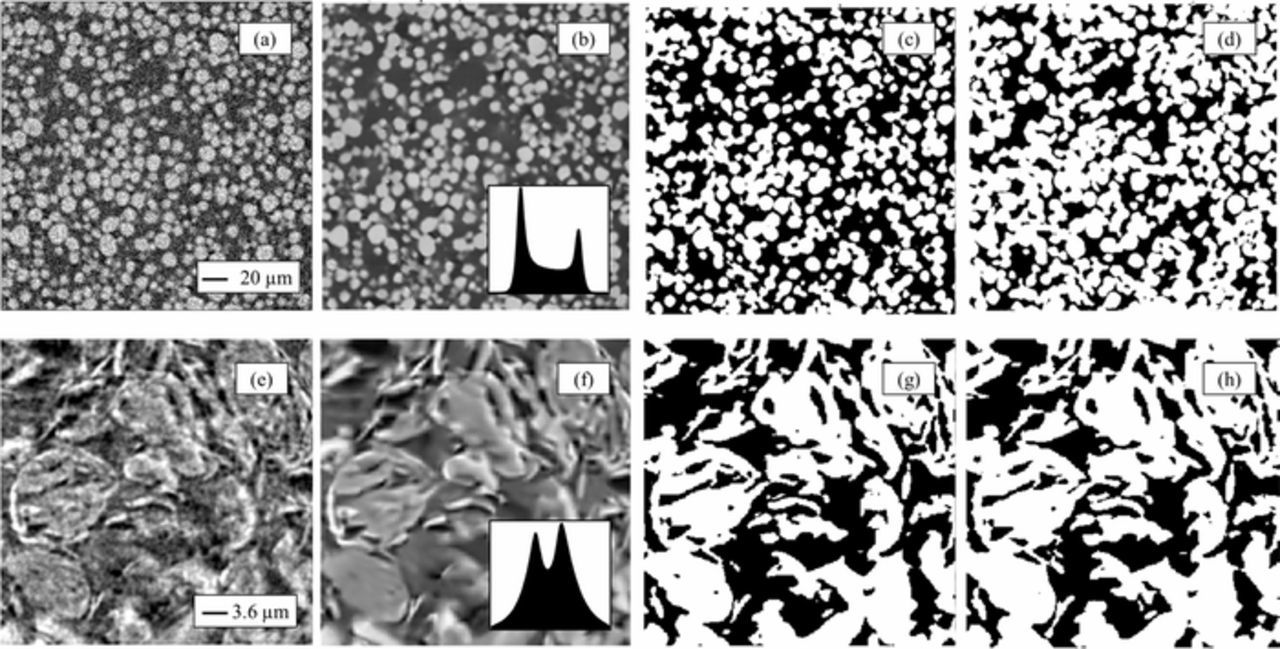
Figure 2. Two-dimensional slice normal to the through-plane direction taken for (a-d) the positive electrode 1-CAL and for (e-h) the negative electrode 5-CAL. The raw and filtered images are shown in (a, e) and in (b, f), respectively. Inserts are the grey-level histogram calculated for the whole volumes. A first automatic segmentation (local Otsu) is performed, which results in a volume fraction for the black phase very close to the sum of pore plus CBD volume: εpore + CBD (c, g). A manual segmentation attributes the black phase with the volume fraction of the pore only: εpore (d, h).
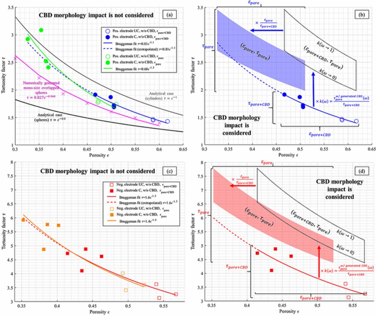
Figure 3. Through-plane tortuosity factor plotted as a function of the porosity, for (a, b) the positive electrodes and (c, d) the negative electrodes. (a, c) The electrodes tortuosities are plotted twice: with a segmentation that matches the pore plus CBD (εpore + CBD), and a second that matches the pore (εpore), each with their respective Bruggeman fit, for both calendered (C) and uncalendered (UC) samples. CBD morphology is not considered, only its impact on the pore volume. The analytical Bruggeman relationships (for spheres and cylinders) are also plotted, as a reference, for the positive electrodes as tortuosities are in the same order. (b, d) The corrective factor k(ω) is applied onto the Bruggeman relationship determined for τpore + CBD = f(εpore + CBD) to deduce the actual pore tortuosity τpore. Porosity values are then shifted so that the transparent area corresponds to the domain τpore = f(εpore). The upper and lower bounds of the areas correspond to the lowest and highest k(ω) values (1.42–1.81 for the positive electrode and 1.35–1.60 for the negative electrode).
Modeling Approach
Microstructure homogenization
A homogenization calculation is the numerical procedure used to derive an effective property from the analysis of the structure at a lower scale, which is then used as an input parameter to macroscale models. Various numerical methods have been developed to calculate the tortuosity factor of a medium.35,38,75 However, they are not necessarily equivalent as some rely purely on a geometric interpretation of the tortuosity while others consist in solving the Laplace equation problem. The geometrical approach provides more insights about the relationships between the tortuosity and the medium morphology but requires the determination of additional parameters (constrictivity and geometric tortuosity) and relationships specific to the investigated microstructures to be accurate,35 which are out of the scope of this paper. In this work we consider only the diffusion approach. The steady state diffusion equation (i.e., the Laplace equation ∇2C = 0, with C being the concentration field) is solved within the connected pore network. A unit diffusion coefficient is attributed to each voxel of the pore domain (i.e., the bulk or dense diffusion coefficient D0 of Eq. 1 is equal to 1 m2.s-1), and the effective diffusion coefficient is deduced from the analysis of the calculated concentration field using the Fick's first law as detailed here.38 The tortuosity factor is then calculated from Eq. 1. Note that this approach assumes lithium ions do not accumulate locally in the microstructure, for instance due to local defects, and does not consider the nonuniform electrochemical reaction that occurs during battery operation across the active material/electrolyte interface.
Two different methods have been employed to solve the Laplace equation. The first one makes use of the open-source MATLAB software package TauFactor, which was developed for the characterization of microstructural data.75 The software allows for quantification of simple metrics such as volume fractions and specific surface areas, as well as offering a steady-state finite difference solver for calculating the effective diffusivity (and therefore the tortuosity factor). The package also contains an automatic representative volume analysis study tool and allows for a local diffusivity to be specified for each phase separately,76 or even voxel-by-voxel. More recently, the custom solver has been modified to operate in the frequency domain, enabling the calculation of complex diffusion impedance spectra.77 The second method uses the software FEniCS,78 a finite element solver used in a previous work.55 One advantage of the FEniCS software is that it allows setting user-defined boundary conditions (BCs) while TauFactor, in its current state, is restricted to fixed BCs (i.e., Dirichlet). Such flexibility is valuable as homogenization calculations are sensitive to the chosen BCs due to some edge effects induced by their application on a limited domain.38,79 This dependence with the BCs must theoretically vanish for infinite volumes for which edged effects would be insignificant. Such effect corresponds to a source of error that should be quantified, as done by several authors,38,55,79 to provide a range of error in the results analysis. Indeed, the response of the representative volume must be independent of the type of boundary conditions, that is an effective (macroscopic) property should be independent from the choice of the boundary conditions as it is an intrinsic, unique, property of the material.79 In this work, tortuosities obtained with FEniCS have been calculated using fixed (i.e., Dirichlet-Dirichlet), mixed (Dirichlet-Neumann), and imposed flux BCs (Neumann-Neumann, with a fixed anchor point in the pore volume to ensure solution unicity). These BCs are applied on the two opposite planes normal to the investigated direction. In case fixed BCs are used, both planes received arbitrary different fixed values so that a concentration gradient will be calculated. In case an imposed flux is chosen, an identical flux must be applied on both opposite faces to ensure a steady solution can exist (i.e., mass conservation must be satisfied). For mixed BCs, there is no restriction for the choice of the fixed and flux values. Besides, whatever the chosen BCs are, an additional zero-flux BC is applied to the four faces orthogonal with the investigated direction and to the interface pore – complimentary volume. Since the complementary volume of the pore is not meshed, this zero-flux BC is implicitly applied. Concentration fields obtained with FEniCS are displayed in Fig. 1c for a negative and a positive electrode. In this work tortuosity factor values obtained from the numerical calculation come from TauFactor if not specified. They will be later compared with those founded with FEniCS. In both methods, we assume a perfect wetting of the electrolyte on the solid phase. Pietsch et al.80 have shown tortuosity factors numerically calculated from the microstructure analysis were highly dependent on pore volume for low porosity microstructures. Therefore, to be reliable such methods must pay special attention to the segmentation process to make sure a clear identification of the pore domain is achieved. As previously mentioned, microstructure reconstruction often lacks the information of the CBD, resulting in an overestimation of the true porosity of the electrode as CBD is undistinguishable from the pore volume. Therefore, a significant limitation of the homogenization method lies in the missing description of the CBD. In this work, this issue is treated by generating a virtual CBD as described in the next section.
Description of virtual carbon-binder domains
The composite electrodes used in LIBs, be they anode or cathode, are primarily composed of three distinct phases5: (i) active material–Li storing phase, (ii) CBD–providing mechanical integrity and electronic conduction, and (iii) pore–electrolyte phase that facilitates ionic transport. Geometrical features associated with active material particles have been widely studied earlier53,65,81–85 such as particle shape, size distribution, and spatial locations. On the other hand, the secondary solids, i.e., the CBD phase, are often not considered. In fact, most of the studies lump the CBD + pore phase together and treat the microstructure as composed of two phases, active material and CBD plus pore. A very recent set of expriments86 proved that even when the material composition is kept constant, variation in CBD phase distribution leads to different performance and capacity fade trends. Based on such arguments, Mistry et al.6 recently proposed a CBD phase description that reproduces different spatial arrangements depending on interfacial energies. CBD phase arrangement around an active particle skeleton results from evaporation stage during electrode preparation. From an initial colloidal slurry containing active particles, conductive additives, binder and solvent, the solvent phase evaporates and leaves behind the microstructure of a composite electrode.86–89 The dynamics of this process are rich and influenced by a multitude of factors, for example, capillary forces that cause heterogeneous solvent evaporation from all the pores. The interfacial energetics dictate the equilibrium preference of CBD distribution and serve as the driving potential for the microstructural arrangement. Given that the energetics is responsible for the spatial preference, the present morphology treatment relies on interfacial energies. Other factors such as drying temperature can change this arrangement dictated purely by thermodynamic factors and result in CBD deposition present in interparticle crevices90 against a fairly delocalized distribution91 that is present everywhere as assumed in the present calculations. Our future work will quantitatively study the differences among CBD distributions that are not covered by the present morphology treatment.
In this work, for a given active material skeleton, the CBD phase can either deposit on the active material surface or on a pre-deposited CBD phase as more CBD is added until the prescribed recipe is achieved. At this stage, there is a competition between two events: adhesion of CBD on the active material and cohesion of CBD on CBD. The energetics of the two events decide which one is more favorable.92 If adhesion is stronger than cohesion, the CBD phase forms a more layered arrangement while for a stronger cohesion, it forms a rather finger-like distribution. Thus, without varying the amount of the CBD phase, its spatial arrangement changes, which in turn affects the microstructural effective properties like active area and tortuosity6 and subsequently alters the electrochemical response of the electrodes. This description allows for a continuous range of CBD morphologies in between two extremes: film-type and finger-like. Each morphology is identified by a dimensionless quantity, ω, referred to as the morphology factor. ω → 0 gives film-type, while ω → 1 leads to finger-like arrangements. Essentially ω correlates with the ratio of cohesive to adhesive energies. Since the actual CBD morphology type has not been established yet for these electrodes (due to limitations of the FIB-SEM technique, as discussed in Computed tomography and segmentation section), CBD generated between these two plausible bounds (ω → 0 and ω → 1) are investigated in this work to provide a comprehensive analysis of the CBD morphology impact on the tortuosity. Tomographic data enhanced with CBD, described in Accounting for the CBD phase on the pore tortuosity section, are available open source.74
Macro-homogeneous modeling
To provide independent validation of the microstructure model tortuosity factor estimate, the graphite/NMC532 electrode library was simulated using a previously reported macro-homogeneous electrochemical model.93 The model uses the pseudo-2D formulation originally proposed by Newman and coworkers.11 Instead of the typical full-cell formulation, the composite negative electrode is replaced with an ideal lithium negative electrode. The lithium potential is set to be the reference potential, and the model assumes facile kinetics at the lithium surface resulting in zero overpotential at the lithium surface. The Li-ion flux entering the electrolyte phase at the lithium-separator interface is implicitly set through the applied electronic current density. The macro-homogeneous model prediction for range of appropriate tortuosity values is based on matching to experimentally measured electrochemical data at the highest achievable rate. For NMC, this is lithiation at 1C and graphite is de-lithiation at 0.5C. The tortuosity range is selected to approximately match the final capacity and to a lesser extent match the voltage profile of those experimentally measured.
All model parameters except tortuosity factor were deduced from fitting to electrochemical data for the baseline NMC (4-CAL in Table I) and graphite (8-CAL) electrodes having thicknesses of 34 and 44 μm, respectively. At these thicknesses and rates ≤ 2C, the macro-homogenous model is not sensitive to the tortuosity factor because electrolyte transport is not limiting. For the thicker electrodes, the tortuosity was then adjusted for each electrode to give a best fit between the experimental and model-predicted rate data. The separator was assumed to have a Bruggeman exponent of 2–2.3 based on microstructure reconstruction values reported in the literature.94,95 A recent study suggested the actual Bruggeman exponent for separators may be considerably higher than that predicted by reconstruction due to difficulty in fully wetting the separator.95 For the thicker electrodes and rates examined, the model-predicted Bruggeman exponent for the working electrode changes by 0.1 or less even if the separator tortuosity factor is doubled.
Model parameters are summarized in Table II. Electrolyte conductivity and diffusivity equations, previously developed based on measurements limited to salt concentrations below 2.2M, have been modified to approach zero conductivity/diffusion near a salt concentration of 4M.13,96 The model equations consider fluxes induced by changes in the electrolyte transference number. For NMC, solid-state diffusivity and exchange current density variation with intercalation fraction were taken from galvanostatic intermittent titration technique (GITT) experiments and analysis.97 Due to challenges in classical GITT analysis for a multi-phase material, a constant diffusion coefficient and exchange current density were fit for graphite based on electrochemical half-cell rate data. The specific surface area of each electrode is based on the classical assumption of isolated spheres and calculated as as = 3εs/rp, where εs is the active material solid volume fraction and rp is the mean active material particle radius. With the diameter and the specific surface area fitted to match the electrochemical data of the thin baseline electrodes (cf. previous paragraph), only one free parameter – tortuousity factor – was fit to the other thicker electrodes. The values given in Table II are approximations for as of calendered and uncalendered electrodes, with the exact value for a particular electrode varying slightly due to small changes of the solid volume fraction.
Table II. Macro-homogeneous model parameters representing graphite and NMC532 electrodes and electrolyte consisting of LiPF6 in EC/EMC (30%:70% by weight) at 30°C. Intercalation fraction is noted x, Electrolyte concentration (in kmol.m−3) Ce in the expressions within the table.
| Properties | Units | NMC 532 | Graphite | Electrolyte | |
|---|---|---|---|---|---|
| Transport properties13,96 | Diffusion Coefficient (Ds) | m2.s−1 | 10^(-2319 × x10 + 6642 × x9-5269 × x8-3319 × x7 + 10038 × x6 -9806 × x5 + 5817 × x4-2286 × x3 + 575.3 × x2-83.16 × x-9.292) | 1.0e-14 | 10^(-4.5227-0.5382/(56.81-6.86 × Ce)-0.1976 × Ce) |
| Ionic Conductivity (κ) | S.m−1 | n/a | n/a | 2.184 × Ce-1.559 × Ce2 + 0.3869 × Ce3-0.0333 × Ce4 | |
| Transference Number (t+Li+) | - | n/a | n/a | -9.076E-4 × Ce2 + 0.01791 × Ce + 0.44196 | |
Activity Coefficient  |
- | n/a | n/a | 1.5985 × Ce2-0.1998 × Ce-0.1934 | |
| Electrochemical reaction, resistance, and concentrations97 | Open circuit potential (U) | V | -3640 × x14 + 13176 × x13-14557 × x12-1571 × x11 + 12656 × x10-2058 × x9-10744 × x8 + 8698 × x7-829.8 × x6-2074 × x5 + 1190 × x4 – 272.5 × x3 + 27.23 × x2-4.158 × x + 5.3147- 5.5732E-4 × exp(6.56 × x^41.48) | U1 = 1.05 × tanh((x + 0.05)/2.492E-5) - 0.163 × tanh((x-0.0205)/0.0181) -0.0778 × tanh((x-5.295E-4)/1.027E-4) - 0.120 × tanh((x + 1.540)/0.0781) -0.0941 × tanh((x-0.1083)/0.0989) -0.01934 × tanh((x-0.5105)/0.01729) + 0.4148 × tanh((x + 1.323)/0.09532) + 0.0245 × tanh((x-0.08858)/0.0258) | n/a |
| U2 = 4.380E-3 × x6 + 1.423E-3 × x5-3922 × x4 + 14715 × x3-20704 × x2 + 12948 × x-3037 | |||||
| U = U1 + (U2-U1)/(1 + exp(-1000 × (x-0.9172))) | |||||
| Exchange current density i0 | A.m−2 | (-70.31 × x6 + 257.7 × x5-381.4 × x4 + 287.7 × x3-113.7 × x2 + 21.51 × x-0.8845) × (Ce/1.2)^0.5 | 1.0 | n/a | |
| SEI film resistance (Rfilm) | Ω.m2 | 0.014 | 0.025 | n/a | |
| Maximum lithium concentration (Cs, max) | kmol.m−3 | 48.9 | 30.0 | n/a | |
| Initial Concentration (Ce) | kmol.m−3 | n/a | n/a | 1.2 | |
| Microstructural Characteristics | Thickness | μm | cf. Table I | 25 | |
| Porosity ɛ | m3.m−3 | cf. Table I | 39% | ||
| Particle Radius rp | μm | 1.8 | 5.15 | n/a | |
| Specific surface area as | m2.m−3 | ∼8.2 × 10⁵ (CAL) ∼6.7 × 10⁵ (UNCAL) | ∼3.3 × 10⁵ (CAL) ∼2.6 × 10⁵ (UNCAL) | n/a | |
| Bruggeman Exponent p | - | cf. Table III | |||
Results
Microstructure homogenization
The through-plane tortuosity factor was calculated with the TauFactor application for the 14 reconstructed volumes. Since the CBD phase is not visible though X-ray tomography, segmentation was performed so that the void phase corresponds to the pore plus CBD, thus the calculated tortuosity is τpore + CBD and provides an underestimation of the actual tortuosity τpore. Results are reported in Table III and plotted in Fig. 3. As expected, calendered electrodes present a higher tortuosity factor compared with the uncalendered ones, whose variation can be fitted through a Bruggeman relationship (cf. Fig. 3). The calendering impact on the tortuosity can be mainly explained simply by the change of porosity. However, the negative electrodes show a much higher through-plane tortuosity factor compared with the positive electrodes for similar porosity values (cf. Figs. 3 and 4), implying positive and negative electrode morphologies are distinct, as visual inspection reveals (cf. Figs. 1a and 2). NMC particles can be considered roughly spherical while graphite particles present flake-like geometries. The impact of such non-spherical geometry on the pore tortuosity factor anisotropy has been investigated by several authors.26,46 To quantify this, the in-plane tortuosity was also calculated. Figure 5a shows the resulting tortuosity factor anisotropy (defined as the ratio between the through-plane tortuosity and the mean in-plane tortuosity). A higher tortuosity factor anisotropy is obtained both for positive and negative calendered electrodes. Thus, calendering impacts the microstructural morphology in addition to the porosity reduction. In addition, negative electrodes show a significant anisotropy that hinders the diffusion through the electrode thickness.
Table III. Volume fractions and tortuosity results obtained from microstructure homogenization τmicro, macromodel fitting τmacro and experimental measurements τexp.
| Through-plane tortuosity τ | |||||||||||
|---|---|---|---|---|---|---|---|---|---|---|---|
| Porosity | Microstructure homogenization | ||||||||||
| Electrode investigated | Composite thickness [μm] | Recipe calculation εth | Segmentation εPore + CBDsegmentation | Tau factor τpore + CBD | FEniCS τpore + CBD | Bounds τpore + CBD | CBD corrective factor k(ω) | τmicro | Macromodel fittingτmacro | Experimental determinationτexp | |
| Positive NMC | 1-UNCAL | 160 | 49.1 | 58.7 | 1.47 | 1.45–1.48 | 1.45–1.48 | 1.42–1.81 | 2.06–2.68 | 2.1 a | 2.07–2.27 |
| 1-CAL | 129 | 36.8 | 49.9 | 1.87 | 1.81–1.86 | 1.81–1.87 | 2.57–3.38 | 2.7–3.7 | 2.92–3.06 | ||
| 2-UNCAL | 140 | 51.8 | 61.7 | 1.43 | 1.42–1.43 | 1.42–1.43 | 2.02–2.59 | 2.1 a | Not tested | ||
| 2-CAL | 108 | 37.5 | 50.6 | 1.72 | 1.71–1.75 | 1.71–1.75 | 2.43–3.17 | 5.0–6.0 b | Not tested | ||
| 3-UNCAL | 106 | 47.4 | 58.7 | 1.45 | 1.45–1.46 | 1.45–1.46 | 2.06–2.64 | 2.1 a | 2.24–2.38 | ||
| 3-CAL | 88 | 36.6 | 50.6 | 1.69 | 1.63–1.68 | 1.63–1.69 | 2.31–3.06 | 1.7–4.5 | 3.69–3.83 | ||
| 4-CAL | 34 | 33.5 | 46.7 | 1.91 | 1.82–2.52 | 1.82–2.52 | 2.58–4.56 | n/a a | 2.47–2.61 | ||
| Negative | 5-UNCAL | 205 | 50.7 | 54.0 | 3.62 | 3.73–4.01 | 3.62–4.01 | 1.35–1.60 | 4.89–6.42 | 5.1–5.8 | 6.24–6.38 |
| graphite | 5-CAL | 165 | 38.8 | 46.2 | 4.62 | 4.44–4.85 | 4.44–4.85 | 5.99–7.76 | 6.6–8.0 | 5.40–5.54 c | |
| 6-UNCAL | 173 | 51.8 | 56.7 | 3.26 | 3.21–3.30 | 3.21–3.30 | 4.33–5.28 | 4.8–5.5 | 6.56–6.70 | ||
| 6-CAL | 131 | 36.3 | 41.5 | 4.73 | 4.49–4.76 | 4.49–4.76 | 6.06–7.62 | 7.5–9.3 | 7.98–8.12 | ||
| 7-UNCAL | 140 | 51.4 | 54.4 | 3.14 | 3.00–3.27 | 3.00–3.27 | 4.05–5.23 | 6.5–7.5 | 5.89–6.03 | ||
| 7-CAL | 110 | 38.0 | 43.5 | 4.11 | 4.01–4.53 | 4.01–4.53 | 5.41–7.25 | 7.5–9.0 | 5.85–5.99 | ||
| 8-CAL | 44 | 38.4 | 44.0 | 4.88 | 4.60–5.18 | 4.60–5.18 | 6.21–8.29 | n/a a | 4.08–4.224.7–5.3 d | ||
aMacromodel not sensitive enough to provide an error estimation. bRelatively poor electrochemical performance of this electrode likely induced an overfitting of the tortuosity factor. cObservation reveals the sample was cracked prior to the experimental measure, biasing the result. dExperimental measure appeared to be less reliable possibly due to sample-to-sample variation. Polarization interrupt method39 applied to two additional samples of this electrode provided higher value (4.7 and 5.3) more in agreement with τmicro.
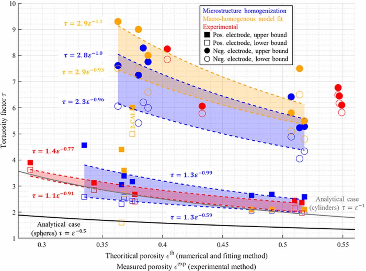
Figure 4. Through-plane tortuosity values comparison for the three methods. The reader is invited to use Table III to identify the samples. Lower and upper bounds of the tortuosity are deduced from the error analysis, and transparent areas correspond to the region between these two bounds. Error range is not displayed for data sets for which (i) not enough points have been obtained (negative electrode, experimental method) and (ii) accurate error estimation was not achieved (positive electrode, macromodel fitting). Porosity values being measured different from the recipe calculation, experimental points are plotted with the measured porosity. Experimental values for samples 5-CAL and 8-CAL are not displayed due to questioned values (discussed in Tortuosity comparison with experiment section). Bruggeman relationship for analytical cases are also plotted for comparison purpose.
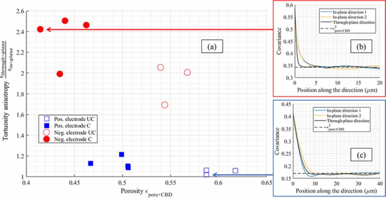
Figure 5. (a) Tortuosity anisotropy plotted as a function of the pore + CBD volume fraction for both positive and negative electrodes. (b) Covariance functions of the negative electrode 6-CAL and (c) of the positive electrode 3-UNCAL plotted for both directions.
Co-variance anisotropy
This high tortuosity anisotropy is correlated with the covariance anisotropy (cf. Fig. 5b). The covariance function55,79  (also called two-point correlation function) is the probability that two points
  and
and  of the domain separated by a vector
  belong to the same phase V, i.e.,
  . It has been analytically established that the covariance function reaches an asymptotic value (equal to the square of the volume fraction) when the distance h (
 ) matches the particle diameter.79 Thus, any anisotropy on this characteristic distance implies an anisotropy on the particle diameter, that suits very well the flake-like visual aspect of the graphite electrodes. The covariance function reveals the in-plane graphite particle sizes are significantly larger compared with the through-plane diameter (cf. Fig. 5b). The graphite particles' largest dimension is preferentially oriented along the in-plane directions, which induces a more tortuous path along the electrode thickness. On the contrary, NMC particles' dimensions are quite isotropic (cf. Fig. 5c) which results in an almost isotropic tortuosity factor (cf. Fig. 5a). For the rest of the article, tortuosity will refer to the through-plane tortuosity factor unless otherwise specified.
Influence of the CBD phase
A critical issue with microstructure homogenization lies in the missing spatial location of the CBD. To overcome this problem in this present work, CBD is numerically generated through a physics-based description to match the volume fraction of the binder and carbon additives. This generation algorithm is explained in Description of virtual Carbon-Binder Domains section and detailed here.6 A key point of the algorithm is to control the preferential deposition of the CBD through a morphology factor ω, that ranges from 0 (preferential deposition on active material surface) to 1 (preferential deposition on existing CBD). While the morphology parameter ω and the porosity are independent, it is expected ω will change the pore tortuosity, at constant porosity, as it affects the pore morphology (which should induce a change on the Bruggeman exponent). A preliminary study was performed to evaluate the change of pore tortuosity that can be attributed solely to the porosity. First, for a given microstructure type without the CBD, the coefficients of the generalized Bruggeman relationship (cf. Eq. 3) are determined by calculating the tortuosity factor for different porosities. Then, the tortuosity factor can be deduced from this relationship for any porosity within the range of the porosities used to determine the coefficients. Second, tortuosity factor values are calculated for the same microstructure type for similar porosity but augmented with the CBD. Finally, the tortuosity factors deduced from the generalized Bruggeman relationship are compared with the tortuosity factors obtained for the geometry with the CBD, each time with the exact same porosity. Differences between the two results will reveal the part of tortuosity change which is not due to the porosity change but to the pore morphology change. This comparison has been performed for the case of spherical particles as a function of the morphological parameter. For this first analysis, such spherical-particle-based stochastic active material skeletons are generated using GeoDict.98,99 In this frame, domains constituted of mono-size overlapping spheres were generated, with porosities ranging from 0.2 to 0.6 with a 0.05 porosity step. Particle sizes have been set equal to the mean particle diameter calculated for the calendered positive electrode 1-CAL (7.4 μm) to be representative of the investigated electrodes. All domains are cubic, and their volumes are equal to 100 × 100 × 100 μm3, ensuring that the investigated volume is representative. Corresponding electrode specifications are summarized in Table IV. The tortuosity factor was calculated for all these volumes, and a generalized Bruggeman relationship (cf. Eq. 3) was fitted: τ = 0.827 × ε− 0.960. The fit as well as the tortuosity factor-porosity points are shown in Fig. 3a. This first analysis provides us with the tortuosity change due to a simple porosity change, for this specific microstructure. For the second analysis, a new volume was then generated following an identical procedure, but with a porosity set equal to the volume fraction sum of the pore and CBD of the electrode 1-CAL (thus, εpore + CBD = 0.368 + 0.138 = 0.506), and its tortuosity factor has been calculated τpore + CBD = 1.575. Note that a similar value was obtained using the previously fitted Bruggeman relationship (1.591) as both structures were generated with the same algorithm, with only a porosity difference. Then, if we assume that an additional volume of the CBD does not change the intrinsic pore morphology, we can re-use the Bruggeman relationship with the actual pore volume 0.368 without modifying the law exponent to deduce the pore tortuosity, τBruggemanpore = 2.159. To test this assumption, the CBD was generated within the active material complementary volume until its volume fraction matched the actual one (i.e., 0.138). Eleven volumes were generated, with a morphological parameter value that ranges from 0.1 to 0.9 (with a step of 0.1) plus two extreme cases (ω = 0.01 and ω = 0.99), and their tortuosity factor τw/generated CBD pore(stands for pore tortuosity factor determined with the generated CBD) were calculated. Results are plotted in Fig. 6 and show a significant difference between τw/generated CBD pore(tortuosity due to porosity change and morphology change) and τBruggemanpore (tortuosity due to porosity change only), thus indicating the former assumption is incorrect. Note that τBruggemanpore is systematically lower than the tortuosity factor obtained with the generated CBD, τw/generated CBD pore, as the Bruggeman relationship systematically underestimates the actual tortuosity factor by assuming an unchanged pore morphology, while the CBD creates smaller pores and blocks pore diffusion paths (especially for high ω value, cf. Fig. 1b). Since experimental observation has shown that the CBD phase exhibits a convoluted nanopore network, thus significantly changing the pore morphology, (cf. Fig. 1a), it is reasonable to consider that τw/generated CBD pore is closer to the actual tortuosity factor than τBruggemanpore. Please note the difference between the two methods is increasing monotonically with the morphological parameter, as a low ω value corresponds to a CBD thin film deposition that does not drastically change the pore morphology (it roughly corresponds to a pore erosion, cf. Fig. 1b). On the contrary, a high ω value results in a fractal-like CBD that significantly changes the pore diffusion paths, closing some of them and reducing the cross-section of other pore paths (cf. Fig. 1b). Thus, the relative difference 100 × (τw/generated CBD pore − τporeBruggeman)/(τw/generated CBD pore − τpore + CBD), for which the numerator expresses the tortuosity change not accounted by the Bruggeman relationship (i.e., not due to the porosity change) and the denominator expresses the tortuosity change induced by both the porosity and morphology change, ranges from 13.4% to 48.9%. Such non-zero values indicate CBD increases tortuosity factor more than can simply be explained by a decrease in pore volume fraction. For the most tortuous CBD, almost half of the tortuosity factor change is not depicted by Bruggeman's correlation. In terms of effective diffusion coefficient, the relative difference applied for the MacMullin number 100 × (Nmw/generated CBD pore − NmBruggemanpore)/(Nmw/generated CBD pore − Nmpore + CBD) ranges from 7.8% to 35.5%. Even though the tortuosity factor and the MacMullin number are the parameters we are investigating, discussing about relative changes of numbers that appear as denominators (cf. Eq. 1, parameters τ and Nm) are not the best way to represent change. Thus, the same relative difference expression has been evaluated for Deff/D0 (i.e., the inverse of the MacMullin number) and for the tortuosity factor inverse 1/τ. It ranges from 4.1% to 19.3%, and from 9.3% to 36.7%, respectively. This preliminary analysis clearly indicates the Bruggeman exponent determined for microstructures without the CBD cannot be reused as-is to estimate the change of tortuosity factor induced by the addition of CBD for the same material. While this result was expected as the Bruggeman exponent is unique for each different microstructure, these results quantify the error when one relies only on the Bruggeman relationship. The significant underestimation is a strong incentive to determine finely the CBD impact on the tortuosity factor and which justifies, in part, this work.
Table IV. Summary of the numerically generated stochastic geometries.
| Active material source | Domain size [μm3] | Volume fraction (pore/active material/CBD) | Particle shape and size distribution | Particle size parametera | Particle orientation vectorb | CBD morphology parameter ω | Number of samples |
|---|---|---|---|---|---|---|---|
| Negative graphite electrode: stochastic generation | 32 × 32 × 32 | 0.38/0.56/0.06 (identical to 5-CAL) | Flake-like, mono-size | a = 1.2 μm, b/a = 1, h/a = 0.2 | [0.33, 0.33, 0.33] | 0.5 | 10c |
| 0.01, 0.1, 0.2, ..., 0.9, 0.99 | 11 | ||||||
| Flake-like, log-normal | a = 1.2 μm, std. dev. = 0.6 μm, b/a = 1, h/a = 0.2 | [0.33, 0.33, 0.33] | 0.01, 0.1, 0.2, ..., 0.9, 0.99 | 11 | |||
| [0.2, 0.2, 0.6] | 0.01, 0.1, 0.2, ..., 0.9, 0.99 | 11 | |||||
| [0.1, 0.1, 0.8] | 0.01, 0.1, 0.2, ..., 0.9, 0.99 | 11 | |||||
| Negative graphite electrode: 7 volumes from X-ray tomography | n/a | n/a | n/a | n/a | n/a | 0.01 & 0.99 | 2 × 7 = 14 |
| Positive NMC electrode: stochastic generation | 100 × 100 × 100 | No CBD, Porosity 0.20, 0.25, ..., 0.60 | Spheres, mono-size | r = 3.7 μm | [0.33, 0.33, 0.33] | n/a | 9 |
| 0.37/0.49/0.14 (identical to 1-CAL) | Spheres, mono-size | r = 3.7 μm | [0.33, 0.33, 0.33] | 0.01, 0.1, 0.2, ..., 0.9, 0.99 | 11 | ||
| Spheres, log-normal | mean r = 3.7 μm, std. dev. = 1.9 μm | [0.33, 0.33, 0.33] | 0.01, 0.1, 0.2, ..., 0.9, 0.99 | 11 | |||
| Positive NMC electrode: 7 volumes from X-ray tomography | n/a | n/a | n/a | n/a | n/a | 0.01 & 0.99 | 2 × 7 = 14 |
aFlake-like particles have three lengths: a – semi major axis, b – semi minor axis, and h – thickness, and are specified in terms of b/a and h/a ratios. bThe particle orientation vector (i, j, k) represents the average direction vector, with (0.33, 0.33, 0.33) meaning isotropic. Averaging is performed over all the particles present in the given volume. cUsed to check CBD generation algorithm reproducibility.
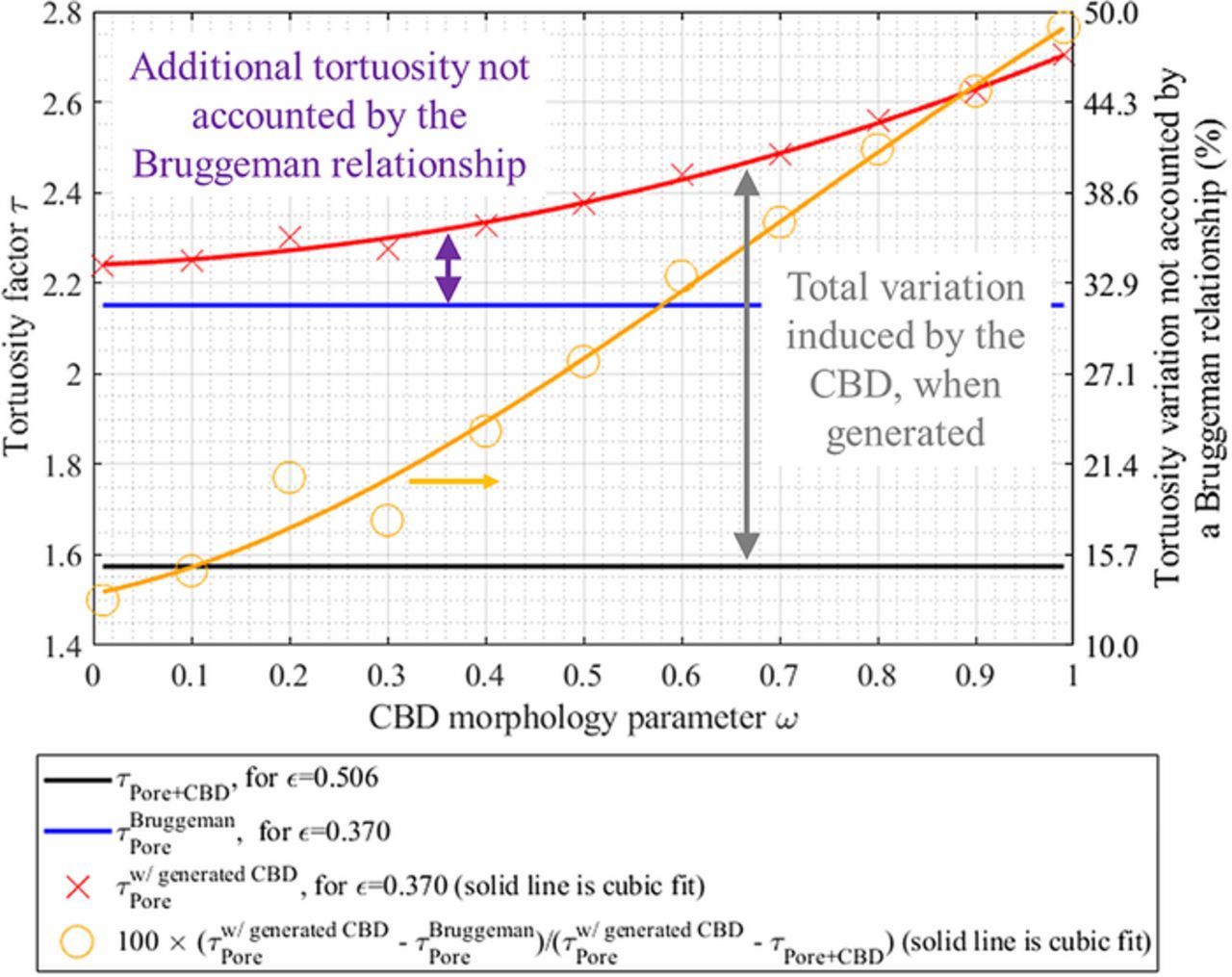
Figure 6. Bruggeman relationship underestimates the tortuosity change induced by the CBD, especially for high ω values. Illustrated with mono-size generated spherical particles. The chosen volume fractions (εpore = 0.368 and εCBD = 0.138) and the particle diameter correspond to the positive calendered electrode 1-CAL.
Accounting for the CBD phase on the pore tortuosity
We define a corrective factor k (cf. Eq. 4a) equal to the ratio of the tortuosity factor calculated on the pore domain only (with the active material and the numerically generated CBD being the complementary volume), τw/generated CBDpore, over the tortuosity factor calculated on the volume that encompasses both the pore and the CBD, τpore + CBD. Such corrective factors can be determined for microstructures for which the three phases (pore, solid material and CBD) are known or generated. Since for typical X-ray tomography the CBD is not distinguishable from the pore domain, the tortuosity calculated for the darkest voxels is actually τpore + CBD. Then, if one multiplies the tomography-based τpore + CBD with this corrective factor, the resulting value will be equal to the actual pore tortuosity τpore if the generated CBD is identical to the actual one, otherwise it will provide an approximation (cf. Eq. 4b). Another interpretation of the corrective factor lies in the multi-scale analysis of the tortuosity factor.29,56 Vijayaraghavan et al.29 have analytically shown that the tortuosity factor of a medium constituted of macro-pores homogenously filled with a nano-pore network is equal to the product of their respective tortuosity factors (i.e., medium tortuosity factor equals to macro-pore tortuosity factor times nano-pore tortuosity factor). According to the multi-scale interpretation, the corrective factor is equal to the nanopore network tortuosity factor if the CBD is uniformly distributed within the (macro) pore, which has not yet been demonstrated (cf. Eq. 4c).
![Equation ([4a])](https://content.cld.iop.org/journals/1945-7111/165/14/A3403/revision1/d0004.gif)
![Equation ([4b])](https://content.cld.iop.org/journals/1945-7111/165/14/A3403/revision1/d0005.gif)
![Equation ([4c])](https://content.cld.iop.org/journals/1945-7111/165/14/A3403/revision1/d0006.gif)
Since CBD generation depends strongly on the morphological parameter ω, then k is a function of ω as well. Fig. 6 shows that the morphology parameter ω has a great impact on the tortuosity factor. Although its effect was evaluated only for a specific microstructure: a domain constituted of mono-size overlapping spheres, which is a major simplification of the actual microstructures. Thus, in this section the corrective factor k was determined for various geometries that mimic the actual positive and negative electrodes. The aim is to provide a range of corrective values that can be applied with confidence to the pore tortuosity factor of battery electrode microstructures when the CBD is not visible.
For the positive electrode, two sets of microstructures consisting of overlapping spherical particles were generated: the first with a mono-size diameter and the second with poly-size diameters. In both cases the parameters are set to mimic the 1-CAL electrode (identical mean diameter and diameter distribution respectively, and volume fractions). For negative electrodes, four sets of microstructures were generated to cover a larger design space as the negative electrode geometry appears to be more complex. The first set consists of elongated flake-like particles, as graphite particles present such stretched out geometries (with a thickness set equal to 0.2 times the two other dimensions, as the covariance analysis, cf. Fig. 5b, suggests a size ratio of around 5:1) of same size with no preferential direction (isotropic case). The second set adds a poly-size distribution with a log-normal size distribution (standard deviation set to 50% of the mean size). The third and fourth sets consider a low and a high particle anisotropy, respectively, controlled through a particle orientation vector. If the major axis of all particles is randomly oriented, the resultant structure is isotropic. In other words, averaged major axis direction vector is (0.33, 0.33, 0.33). Low anisotropy refers to a slight deviation from this, i.e., (0.2, 0.2, 0.6), while high anisotropy corresponds to an average direction vector (0.1, 0.1, 0.8). Here the average is taken over the direction vectors for all the particles. All four sets use the volume fractions of the 5-CAL negative electrodes. Parameters of the generated volumes are summarized in Table IV. For each set, 11 volumes were generated, with morphological parameter ranging from 0.1 to 0.9 (with a step of 0.1) plus two extremes cases (ω = 0.01 and ω = 0.99). For each ω value, τw/generated CBDpore was calculated and thus the corrective factor k(ω). Note that τpore + CBD needed to be calculated only one time per set, as it was independent of ω. Besides, the reproducibility of k(ω) has been checked on the first volume set, by generating 10 times the CBD with an intermediate value of ω = 0.5 (cf. Table IV). It was found that the standard deviation calculated for these 10 iterations was lower than 0.5% of the mean value. This ensured the CBD generation algorithm provided a very similar effective tortuosity for a given value of ω.
Figure 7a plots the calculated corrective factors k(ω). The general trend was a monotonical increase of the corrective factor with ω, for the same reason that explains the increasing trend of Fig. 6. For the positive electrode, the corrective factor ranges from ∼1.42 to 1.81 and depended mainly of the morphological parameter rather than the type of microstructure investigated (mono-size or poly-size spherical particles). For the negative electrode, the corrective factor ranges from ∼1.35 to 1.60 and increased slowly with the morphological parameter ω, except for its largest values in the isotropic mono-size case. These higher values were recalculated (i.e., CBD domain were re-generated) to check their relevance and very similar values have been obtained. Without these two extremes values, the corrective factor would have ranged from ∼1.35 to 1.48. Despite the various geometries generated, associated with very different τw/generated CBDpore values (from 2.23 to 2.87 for the positive electrodes, and from 3.4 to 15.4 for the negative electrodes) the corrective factor was contained in a relatively narrow range for both electrodes (∼1.35 to 1.81). This desirable characteristic was derived from its definition (a ratio) that tended to make it generic, ideally whatever the investigated structure is. Its range could have been further reduced if an estimation of the morphological parameter was reached. However, the determination of the morphological parameter would require additional experimental observations and is out of the scope of the present work. Please note that for both electrodes the corrective factor did not show any anisotropy. It means both in-plane and through-plane tortuosity factors were affected by the generated CBD in a qualitatively similar fashion, and thus the initial tortuosity factor anisotropy, if any, was not affected by the CBD. The isotropy of k was expected since the generation algorithm did not use any preferential direction, ensuring the CBD morphology exhibits isotropic properties. It was checked that the tortuosity factor anisotropies shown in Fig. 5 are very similar either considering τpore + CBD or τw/generated CBDpore.
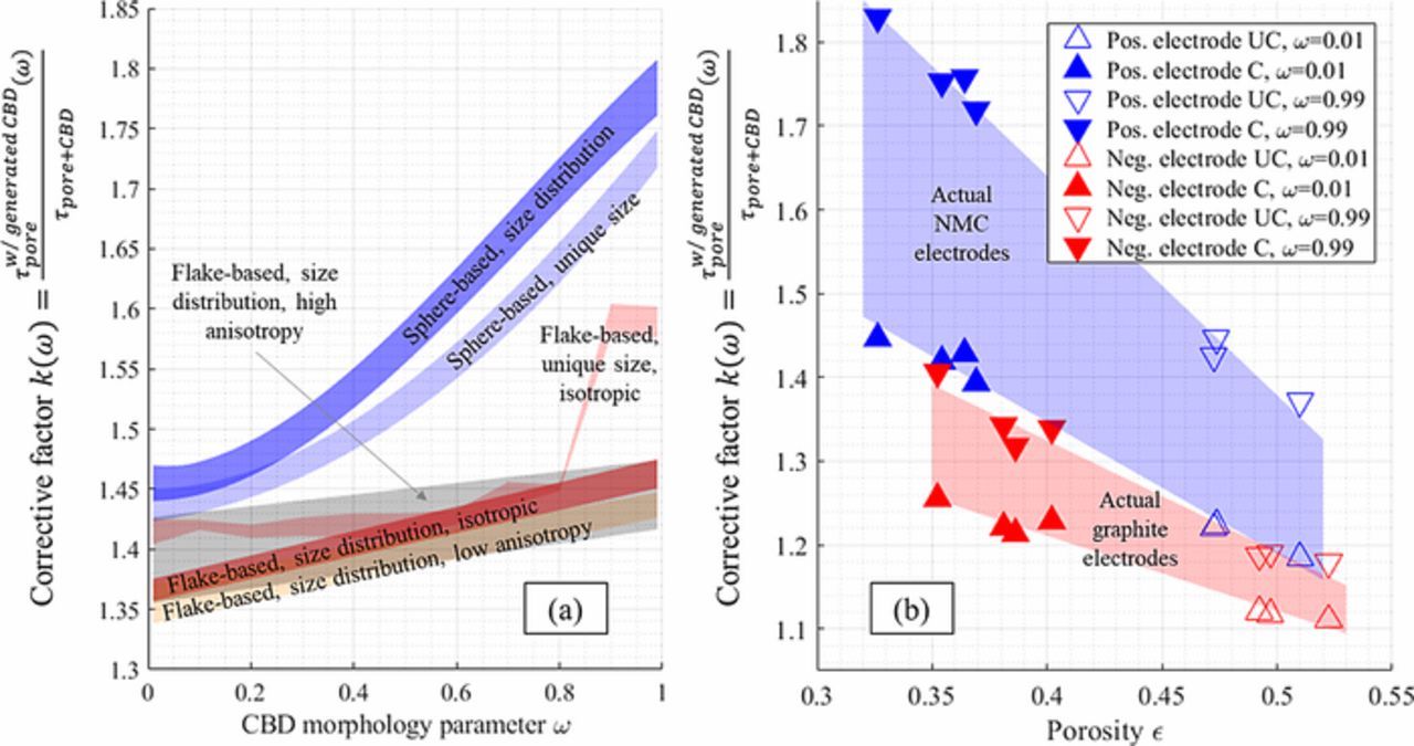
Figure 7. (a) Corrective factor k calculated for various particle morphologies as a function of the CBD morphological parameter. Transparent area represents the minimum and maximum corrective factor calculated along the three directions (cubic and linear fit have been used to determine the areas bounds, except for the flake-based, unique size, isotropic case where no fit has been employed due to the two last high values obtained for ω = 0.9 and 0.99). Other microstructure parameters (volume fractions and particle diameter) correspond to calendered electrode 1-CAL for the sphere-based and to 5-CAL for the flake-based morphologies. (b) Corrective factor calculated for the 14 tomography-based samples volumes, each with ω = 0.01 and ω = 0.99.
Given the generic characteristic of the corrective factor k, the latter was applied to the tortuosity factor τpore + CBD calculated on the actual NMC and graphite electrodes to provide a better estimation of the actual pore tortuosity τpore. An upper bound and a lower bound of 1.42–1.81 and 1.35–1.60 were used for k for the positive and negative electrodes, respectively (cf. Fig. 7a). Results are plotted in Fig. 3. The uncorrected tortuosity factors obtained for both segmentations are also displayed. Adjusting only the segmentation threshold value to match either the volume fraction of the pore or the volume fraction of the pore plus the CBD did not change significantly the Bruggeman exponent (cf. Figs. 3a and 3c), which implies that a similar pore network was investigated in both cases, only with a difference of porosity. Besides, re-using the Bruggeman exponent determined for the microstructure without the CBD leads to a significant underestimation of the pore tortuosity, once the CBD morphology impact is considered (cf. Figs. 3b and 3d). Such a result was expected, as already discussed in Influence of the CBD phase section (cf. Fig. 6). In addition, the analytical Bruggeman relationship were plotted in Fig. 3a for comparison purpose with the NMC spherical particles. The uncorrected tortuosity factor values were higher than the analytical relationship τ = ε− 0.5 (which is only valid for mono-size spherical particles) but lower than the second analytical relationship τ = ε− 1 (which is valid for mono-size cylinders). Such hierarchy suggests the positive electrode particle network's complexity and tortuosity was bounded by those of spheres and cylinders networks. Besides, the numerically generated mono-size spherical particles exhibited a pore tortuosity higher than the analytical case τ = ε− 0.5 but lower than the actual microstructure. Such hierarchy indicates the allowed particle overlapping of the numerically generated volumes induced enough heterogeneity to be higher than the ideal case, but not enough to match the heterogeneity of the actual microstructures. The analytical relationships have not been compared with the negative electrode as the highly non-spherical graphite particles would make such comparison irrelevant.
CBD has also been numerically generated within the pore domain of the 14 tomography-based electrode samples. For each volume, morphological parameter ω = 0.01 and ω = 0.99 have been used to check the lower and upper bounds respectively. These 28 volumes complemented with CBD are available open-source.74 Figure 7b shows the calculated corrective factors. In the investigated porosity range, both its value and its sensitivity with the morphological parameter is decreasing with the porosity. Such trends are derived from the higher volume fraction ratio εCBD/εpore + CBD found for the calendered electrodes. The relative pore volume reduction induced by adding a fixed volume of CBD is higher for low porosity electrodes and explains the corrective factor decrease with porosity for a given CBD morphology. Besides, for a fixed CBD volume fraction, the smaller the pore domain is, the higher the probability a random pore of the electrode being filled with CBD. Thus, the CBD morphology's impact on pore tortuosity factor is more significant for low porous electrodes. This result indicates optimizing the nanopore network geometry of the CBD could be valuable to improve electrolyte transport properties of high energy density electrodes. Although, such optimization study should consider both the tortuosity factor and the specific surface area, as some CBD geometries that minimize the corrective factor (in this work, CBD thin surface layers generated with ω = 0.01) also minimize the specific surface area. The corrective factor bounds determined for the positive calendered electrodes (1.39–1.83) are very close with the ones calculated with the stochastically generated sphere-like microstructure with similar porosity (1.42–1.81). However lower values have been obtained with the calendered negative electrodes (1.21–1.41) compared to the stochastically generated flake-like microstructures. The particle size distribution for graphite is difficult to characterize as it has multiple attributes (unlike spherical NMC system that can be expressed as a histogram of particle diameters) and in turn makes it difficult to stochastically generate equivalent geometries, which explain this discrepancy. For the rest of this work, the bounds determined with the numerically generated microstructures are considered, as they have been obtained on well-defined geometry which are thus easier to reproduce for other groups.
Electron conductivity
This paper mainly focuses on ionic tortuosity, as lithium ion transport in the electrolyte most often limits high C-rate performance. It is often implicitly assumed that electron conductivity is never rate-limiting. To achieve this goal, the conductive carbon phase must have good-enough transport properties namely, high-enough percolation and low-enough tortuosity factor. The CBD tortuosity factor and percolation have been calculated firstly for a generated microstructure consisting of mono-size spherical particles. The chosen volume fractions (εpore = 0.368 and εCBD = 0.138) and the particle diameter correspond to the positive calendered electrode 1-CAL. Results are shown in Figure 8. CBD tortuosity factor increases with the CBD morphology parameter, from ∼5 (for a film-like CBD) to 11.5 (for a finger-like CBD) while CBD percolation slightly decreases from ∼99.7 to 98.1%. In terms of effective transport, it corresponds to very high MacMullin numbers, ranging from 36 to 86, due to the limited volume fraction of the CBD. The percolation value corresponds to the volume of the largest connected CBD volume (or cluster) expressed in percentage of the total CBD volume. Details of the percolation calculation can be found there.38,55 The high percolation indicates a path exists across the electrode thickness to transport the electrons (assuming each voxel of the CBD contains conductive carbon). CBD exhibits an isotropic tortuosity factor (cf. Fig. 8) since the physics-based algorithm used for its generation does not rely on any preferential direction. The impact of the morphology parameter is significantly higher for the CBD tortuosity factor τCBD (+ 130%, cf. Fig. 8) than for the corrective factor k applied to the macro-pore tortuosity factor τpore + CBD (+ 23%, cf. Fig. 7a). It is worth noting the corrective factor is not the CBD tortuosity factor (it can only be compared with the tortuosity factor of the nanopore network embedded within the CBD, cf. Eq. 4c), thus explaining the difference.
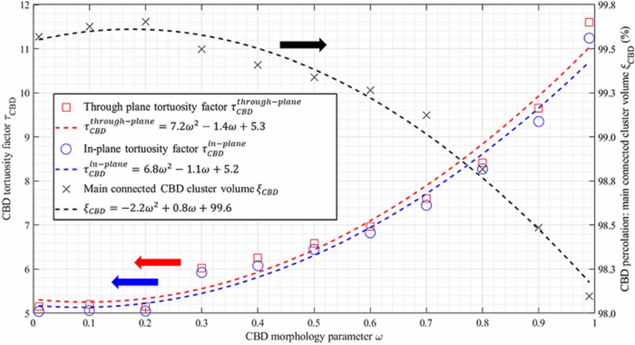
Figure 8. Carbon-Binder Domain (CBD) tortuosity factor and percolation calculated for a stochastically generated microstructure constituted of mono-size spherical particles. Volume fractions (εpore = 0.368 and εCBD = 0.138) and particle diameter correspond to the positive calendered electrode 1-CAL.
Representative volume elements of the CBD are roughly similar with those of the macro-pore domain (i.e., pore and CBD combined). Indeed, for the volume fraction: CBD RVE size is 31 × 31 × 31 μm3 (independent of ω) while macro pore RVE size is 40 × 40 × 40 μm3. And for the tortuosity factor: CBD RVE size ranges from 46 × 46 × 46 μm3 (with ω = 0.01) to 50 × 50 × 50 μm3 (with ω = 0.99) while macro pore RVE size is 42 × 42 × 42 μm3. RVE sizes have been determined following the method described in Reference 55. Note that the CBD RVE sizes are very high compared with the CBD mean particle size. Indeed, the CBD particle equivalent diameter (calculated according to a spherical assumption55) is around 0.55 μm, whatever ω is. Then, the RVE edge lengths are 56 to 91 times this characteristic size, while lower values are expected.55 Comparatively, the macro-pore RVE edge length for the porosity (respectively, the tortuosity factor) is only 9.1 (respectively, 9.5) times the mean pore size, which is the awaited order of magnitude. Such high discrepancy between the RVE and particle size for the CBD indicates the RVE sizes of the CBD nano skeleton depend mainly on the heterogeneity of the spatial arrangement of the higher-scale skeleton which embed it. It implies future three-dimensional imaging of the CBD, to be statistically representative, should have a field of view equal or larger that the RVE of the macro-pore and active material. Such requirement is technically challenging as it implies that both a large field of view and a very fine image resolution are necessary. Although, this result has been obtained with a numerically generated CBD and thus has to be confirmed with an actual image.
CBD through-plane tortuosity has been calculated for the 7 tomography-based NMC electrodes, for the two extremes of the ω morphology parameter (cf. Fig. 9). Tortuosity factor values calculated with the 1-CAL are similar with those obtained on the stochastically generated active material skeleton which share the same volume fraction and solid particle mean size. Besides, RVE sizes are similar with those obtained with the generated skeleton: 27 × 27 × 27 μm3 (independent of ω) for CBD volume fraction, from 40 × 40 × 40 μm3 (ω = 0.01) to 60 × 60 × 60 μm3 (ω = 0.99) for CBD tortuosity factor, and 40 × 40 × 40 μm3 for macro-pore volume fraction and tortuosity factor. Such good agreement indicates the stochastic algorithm mimics fairly well the spatial heterogeneity of the active material skeleton and that the 100 × 100 × 100 μm3 field of view is a relevant choice to investigate such sphere-based calendered electrodes as it is large enough to determine RVE sizes. The CBD tortuosity factor relative increase with the morphology parameter ranges within a relatively narrow range, from + 151 to + 175% (+ 118% if the thin baseline is considered), cf. Fig. 9. This result confirms that the morphology parameter dramatically changes the CBD tortuosity factor, much more than the corrective factor k. CBD percolations for uncalendered NMC electrodes range from 97.3 to 99.2% for ω = 0.01 and from 91.7 to 96.1 for ω = 0.99. For calendered NMC electrodes, CBD percolations are slightly higher (likely due to a higher active material density) from 99.6 to 99.8% for ω = 0.01 and from 97.2 to 98.2 for ω = 0.99.
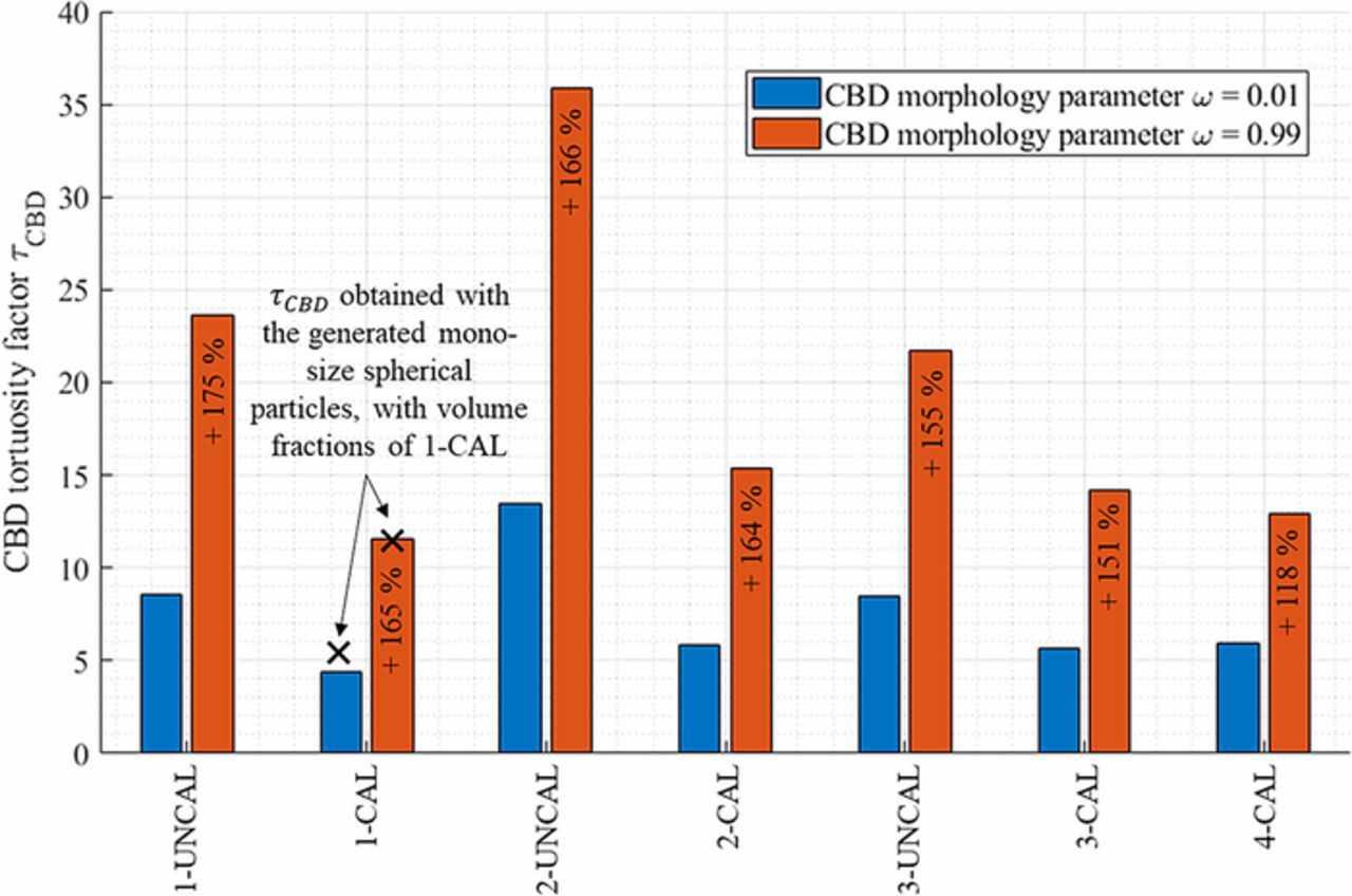
Figure 9. CBD through-plane tortuosity calculated for the 7 tomography-based NMC electrodes, for the two extremes ω morphology parameter (film-like CBD with ω = 0.01, and finger-like CBD with ω = 0.99). Percentages within the bar indicate the relative increase calculated from the reference tortuosity value obtained with ω = 0.01 to the larger value obtained with ω = 0.99.
Finally, the CBD embedded within the graphite does not form a large unique connected cluster but instead forms a multitude of isolated clusters for both the stochastically generated and the tomographic-imaged graphite geometries. This result suggests the smaller CBD volume fractions for the graphite (4.6–6.0% versus 10.6–14.6% for the NMC, cf. Table I) are below the percolation threshold for this particular nanoskeleton, within these particular graphites. With no percolation achieved on this phase, it is not possible to determine its tortuosity factor. Future work could investigate the CBD percolation threshold. Experimentally determined conductivity should show a jump in conductivity when percolation along the electrode thickness is achieved which would provide an interesting point of validation for the numerical characterization.
Other sources of error
Independent from the CBD impact on the tortuosity factor, another source of numerical error is the homogenization numerical calculation itself. In this work the tortuosity factor values obtained with TauFactor (finite-difference-based method) with fixed BCs were compared with those obtained with FEniCS (finite-element-based method) with a set of BCs described in Microstructure homogenization section. In addition, both linear and quadratic basis functions were used with the finite element solver. Results are shown in Fig. 10 and in Table III. The higher the tortuosity factor, the higher the relative difference between the two methods. For microstructures that exhibit relatively low tortuosity values (such as the positive NMC electrodes), the difference between the two methods is contained below ∼9% (6% if FEniCS is used with a quadratic interpolation). For more tortuous structures, such as the negative graphite electrodes, the relative difference is higher and reaches 17% (10% if FEniCS used quadratic interpolation). A more comprehensive comparison between the two methods is provided in the appendices, including a comparison of their dependence on voxel size. To quantify the error induced by the choice of the numerical method used to solve the homogenization problem, the minimum and the maximum τpore + CBD values obtained with either TauFactor or FEniCS (considering only the quadratic interpolation which is more accurate) were retained. They were then multiplied with the corrective factor k so that the final tortuosity value considered from the microstructure homogenization was bounded between min (τFEniCSpore + CBD, τpore + CBDTauFactor) × min (k(ω)) and max (τFEniCSpore + CBD, τpore + CBDTauFactor) × max (k(ω)). The resulting bounds are available in Table III and will be compared with the other techniques (micromodel fitting and experimental).
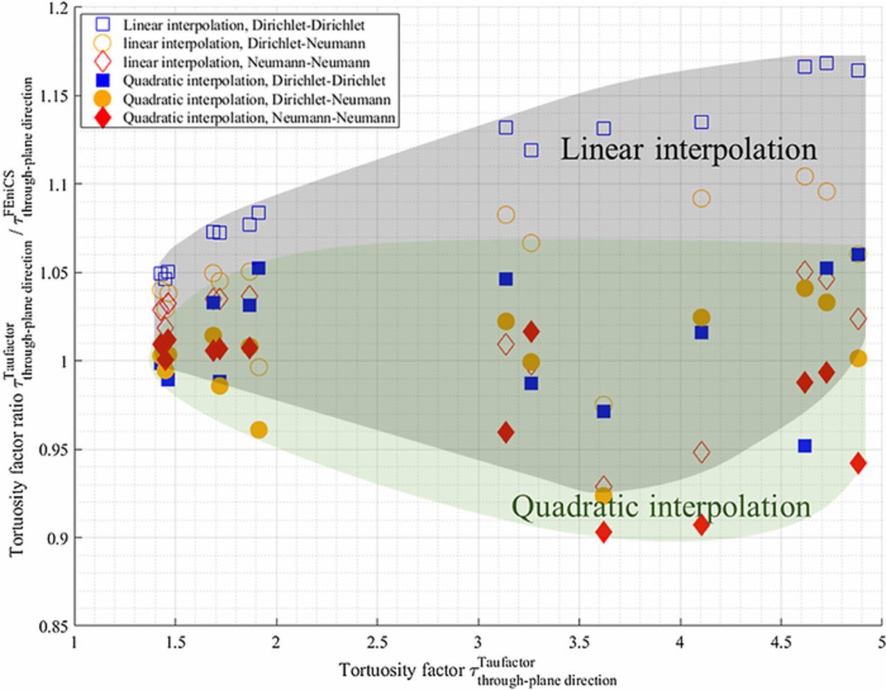
Figure 10. Ratio between the tortuosity factor calculated with TauFactor (finite difference method, fixed BCs) and FEniCS (finite element method) as a function of the tortuosity factor (TauFactor being used as reference). Fixed, mixed, and Neumann BCs, with either linear or quadratic interpolation have been tested with FEniCS. The gray transparent area contains the ratio obtained with the linear interpolation while the green one contains those calculated with the quadratic interpolation (which is more accurate).
Lastly, the error analysis should also incorporate the porosity error induced by an incorrect segmentation or a non-representative investigated volume. While the pore representative volume of the microstructure was checked, the accuracy of the segmentation is unknown. Considering that the automatic segmentation manages to retrieve the correct volume fraction sum of the CBD and the pore, the segmentation can be considered trustworthy. Nevertheless, it has to be pointed out that an error in the porosity can have a dramatic impact on the tortuosity, especially for the low-porosity materials.80 The highest sensitivity for the low porosity region is derived from the exponential form of the tortuosity factor-porosity relationship as expressed in the classic Bruggeman correlation. To illustrate it, the slope of the tortuosity factor deduced from the Bruggeman correlation has been calculated for the 14 electrodes. The actual porosity (from recipe calculation) and the mean Bruggeman exponent (from the numerical bounds) obtained with the homogenization calculation have been used to calculate the instantaneous slope. For both the positive and the negative electrodes, the (absolute) slope is decreasing with the porosity, meaning the calendered electrodes are more sensitive to segmentation error. A plausible error of 0.01 for the porosity translates to an error in tortuosity of ∼0.1 and ∼0.35, respectively, for the positive and negative calendered electrode according to Fig. 11. It is essential therefore to achieve a realistic segmentation to limit this error.
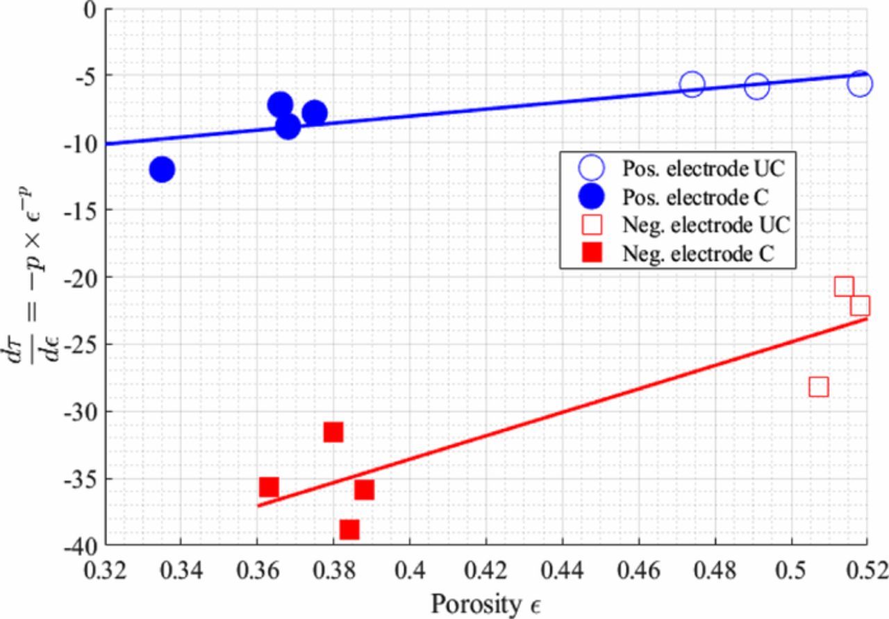
Figure 11. Tortuosity slope calculated for each 14 volumes with their porosity (from recipe calculation) and their Bruggeman exponent (from numerical homogenization, considering the mean value).
Macro-homogeneous modeling
In regards with this effective ionic transport-centered work, the macro-homogenous electrochemical model is used to assess the validity of the microstructure enhanced with CBD characterization approach by fitting the tortuosity factor to electrochemical rate data.
Figures 12a, 12b illustrate 1C discharge curves for the macro-homogeneous half-cell model for calendered NMC cathodes with a thickness of 88 μm (3-CAL) and 129 μm (1-CAL). Each continuous line represents the macro-homogeneous model run with a different Bruggeman exponent/tortuosity. The experimentally measured performance is plotted as discrete points. For a cathode thickness of 88 μm and using electrolyte properties of Table II, increasing the tortuosity was shown to lead to a slight increase in overpotential up to a Bruggeman exponent of 3 (tortuosity of 7.5). However, the discharge capacity was essentially unchanged for this range of tortuosity for the 88 μm cathode. The experimental data fits well with a Bruggeman coefficient between 1.5 and 2.5, which corresponds to a tortuosity of 1.7–4.5. A Bruggeman above 2.5 leads to a significant under-prediction of the discharge plateau. For the thicker 129-μm cathode, the tortuosity had a more pronounced effect on the discharge curve as electrolyte transport becomes more rate limiting. As the Bruggeman coefficient was increased above 2.3 (tortuosity 3.7), the model showed a rapid decrease in the predicted discharge capacity. The experimental data indicated that a Bruggeman exponent of ∼2–2.3 (tortuosity 2.7–3.7) is appropriate. However, the experimentally measured voltage profile and model prediction show significant differences. The cause of the lower experimentally measured starting voltage for the 129 μm thick NMC is uncertain. Presumably, a 100% SOC was reached due to C/10 charging prior to starting the discharge. The mismatch could be due to challenges associated with fabricating thicker electrodes, an unexpected high ohmic resistance from coin cell fabrication, or uncertainties in electrolyte properties at higher salt concentrations. For the 129-μm electrode, the model also overestimated discharge voltage for C/5 and C/2 discharge (cf. Fig. 12d). The predicted discharge voltage for the 88-μm cathode matches the experimental data well at all three rates (cf. Fig. 12c).
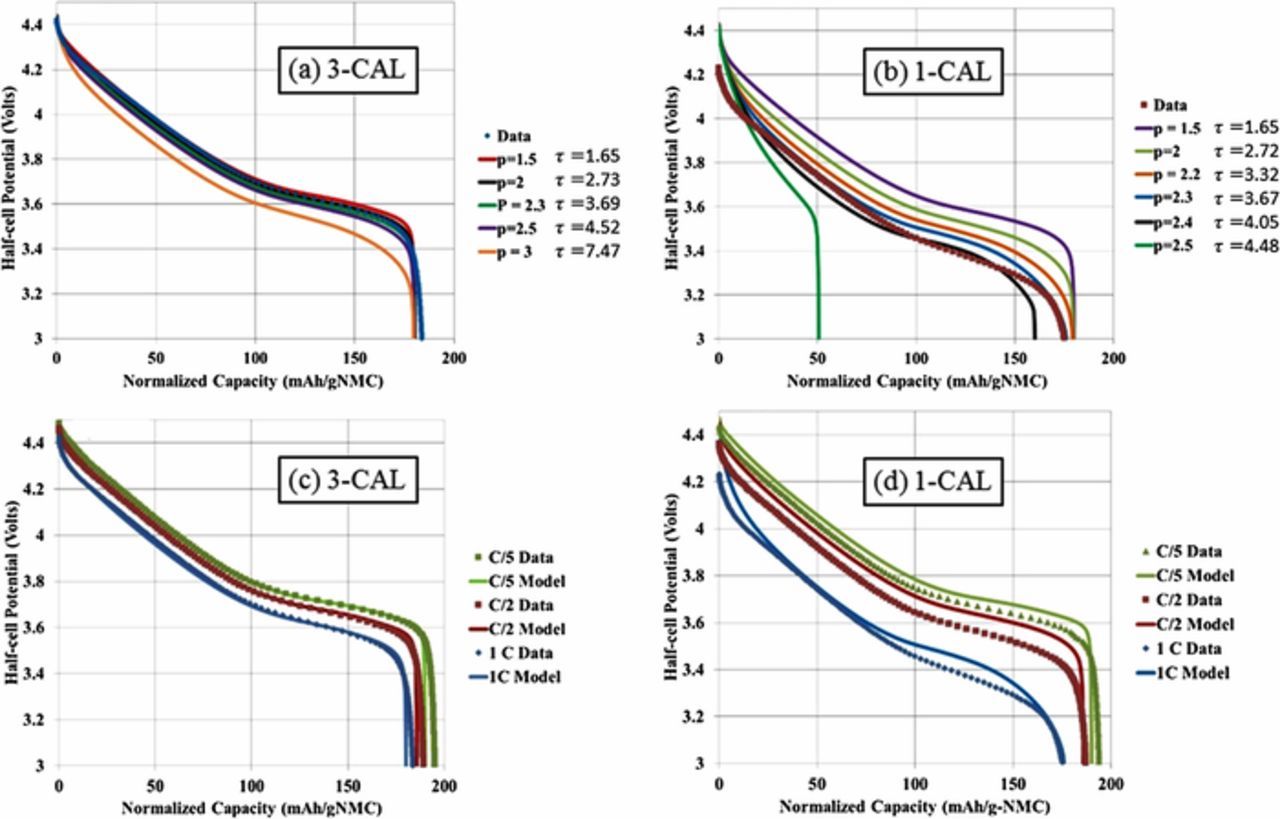
Figure 12. Discharge profiles for half-cells with calendered NMC electrodes of (a, c) 88 μm (3-CAL) and (b, d) 129 μm (1-CAL) calculated with the macro-homogeneous model at 30°C. (a, b) Plotted with different Bruggeman exponents at 1C. (c, d) Discharge profiles displayed at 0.2C, 0.5C, and 1C. The macro-homogeneous model is run with p = 2 and p = 2.3 for the 88- and 129-μm NMC electrodes.
The macro-homogenous model was also used examine the effects of Bruggeman exponent/tortuosity on thick graphite anode performance during de-lithiation, which corresponds to discharge in a full-cell configuration (Figure 13). The macro-homogenous model is run for a 110 μm (7-CAL) and 165 μm (5-CAL) calendered graphite anode half-cell. A tortuosity of 7.5–9 (Bruggeman exponent p of 3.1–3.3) for the 110 μm electrode and 6.6–8 (Bruggeman exponent p of 3.0–3.2) for the 165 μm electrode match the data reasonably well. The higher tortuosity for the anode compared to the NMC cathode is due to the higher aspect ratio particle morphology of the graphite. At 165 μm, the model significantly under predicts the voltage profile. It is not known if this is due to underpredicting voltage losses from electrolyte transport, neglecting multi-phase intercalation physics of graphite, or from challenges in fabricating thicker electrodes.
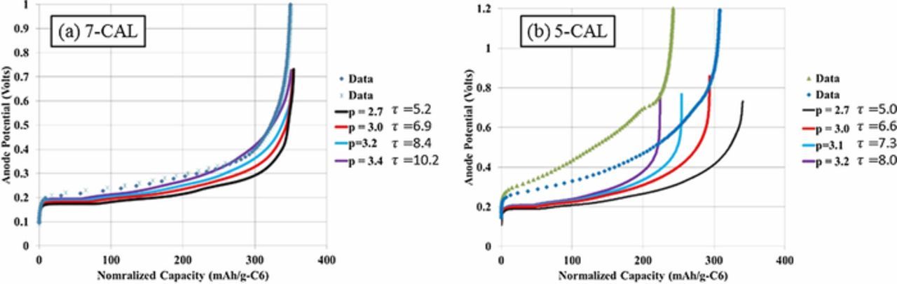
Figure 13. Voltage profiles for graphite half-cells during 0.5C de-lithiation at 30°C for calendered electrodes of (a) 110 μm (7-CAL) and (b) 165 μm (5-CAL). Experimental data have been replicated twice for each electrode using two pouch cells.
In addition, it has been checked the fitted tortuosity factor allowed to correctly estimate with the macro-homogenous model the electrode critical thickness, defined as the threshold value for which higher thicknesses induce a loss in capacity (cf. Figs. 14 and 15, respectively for the cathode and for the anode). Figure 14 illustrates model predictions for 1C discharge capacity and average discharge voltage (defined as the ratio of the discharge energy in Wh over the discharge capacity in Ah) versus NMC cathode thickness (1-CAL 129 μm, 2-CAL 108 μm and 3-CAL 88 μm). The experimentally measured values for the three cathodes are shown as orange dots. The model predicts the discharge capacity is relatively uniform until a critical thickness is reached, after which the discharge capacity rapidly falls off. This critical thickness is decreasing with the tortuosity factor, indicating it is a key parameter to manufacture thick electrodes with high-energy density. The steepness of the falloff in capacity after the critical thickness is a strong function of the electrolyte properties near saturation, which have not been experimentally measured. That is, the electrolyte concentration near lithium electrodes rises rapidly during discharge (close to its saturation value) and leads to a large voltage drop which limits electrode capacity. Experimental data for the limited thickness range seem to be linearly decreasing with thickness. The small change in the experimentally measured discharge capacity for thicker electrodes may be due to fabrication challenges (cracking, isolated clusters, etc.). Fall-off in normalized capacity with thickness will be different in a full-cell configuration with a porous negative electrode. It should be noted that the model was initially formulated and validated for cases where electrolyte transport was not strongly limiting performance (thinner, more porous electrodes; lower rates). Due to these reasons, leaving the tortuosity as an empirical fitting parameter for the macro-homogenous model can be problematic. Ideally reconstruction/direct experimental techniques should be used in conjunction with macromodel to estimate the tortuosity, as proposed in this work.
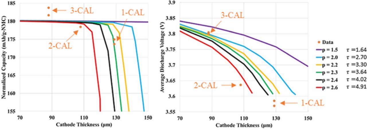
Figure 14. Normalized capacities (left) and average discharge voltage (right) for 1C discharge as a function of cathode thickness for 1-CAL, 2-CAL, and 3-CAL. Model is run with different Bruggeman exponents and porosity set to 37%.
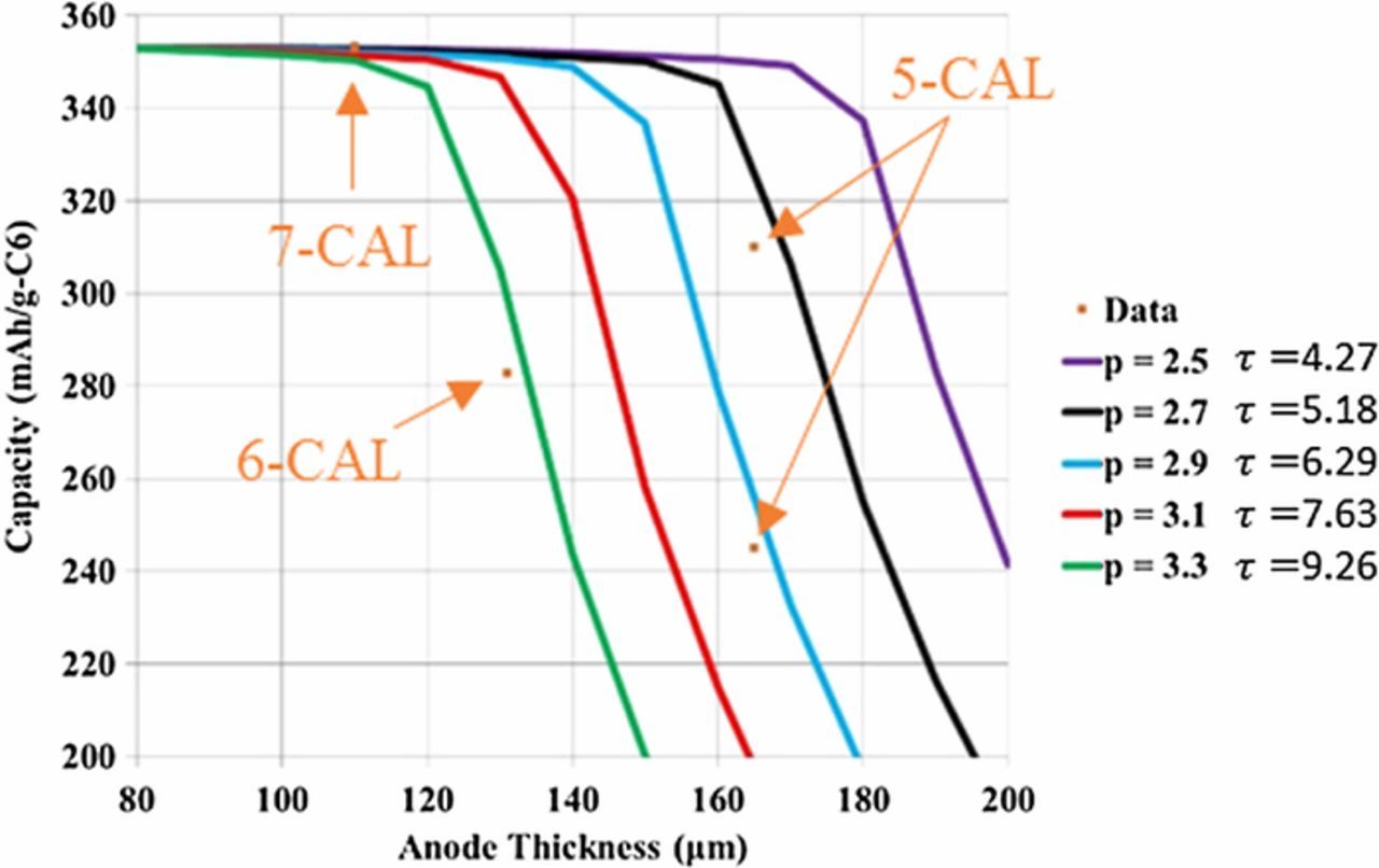
Figure 15. Normalized capacities for 0.5C de-lithiation as a function of anode thickness for 5-CAL, 6-CAL, and 7-CAL. Model is run with different Bruggeman exponents and porosity set to 38%. Note, the data at 165 μm were measured at ∼0.4C (lower capacity is expected at 0.5C).
The experimentally measured and model predicted half-cell delithiation capacities at 0.5C for graphite electrodes (5-CAL 165 μm, 6-CAL 131 μm and 7-CAL 110 μm) are shown in Figure 15. The data are plotted as orange squares and each line represents model predictions with differing tortuosity values. The model-predicted capacity starts rapidly decreasing with thickness as the electrolyte concentration near the lithium surface goes to zero and electrolyte conductivity goes to zero. This falloff is slower for the graphite half-cell than for the NMC cathode due to lower rate (0.5C versus 1C), and the electrolyte diffusion coefficient is high for electrolyte depletion and low for saturation. There is a large spread in capacity measured for two half-cells at 165 μm (cf. Fig. 13b). For this thick electrode, slight differences in the tortuosity of the two samples could result in large differences in charge capacity, indicating a precise determination of the tortuosity is required to provide predictive results.
Lastly, the macro-homogeneous model is used to better understand how 1C discharge performance can be improved for the 129-μm thick cathode, focusing only on the transport properties. The left plot in Figure 16 illustrates model predictions for 1C discharged with enhanced electrolyte transport. Conversely, the right plot in Figure 16 illustrates enhancements in solid-state diffusion. The green line in each plot illustrates the infinitely slow/theoretical discharge curve, and the black lines are the nominal discharge curve using the baseline parameters. Increasing the solid-state diffusion by an order of magnitude through improve diffusion coefficient/reducing particle size results in only a very slight improvement in discharge performance. Reducing the Bruggeman coefficient or increasing the electrolyte diffusion coefficient (De) results in significant rise in discharge voltage, indicating optimizing ionic transport property (i.e., pore tortuosity) is worthwhile.
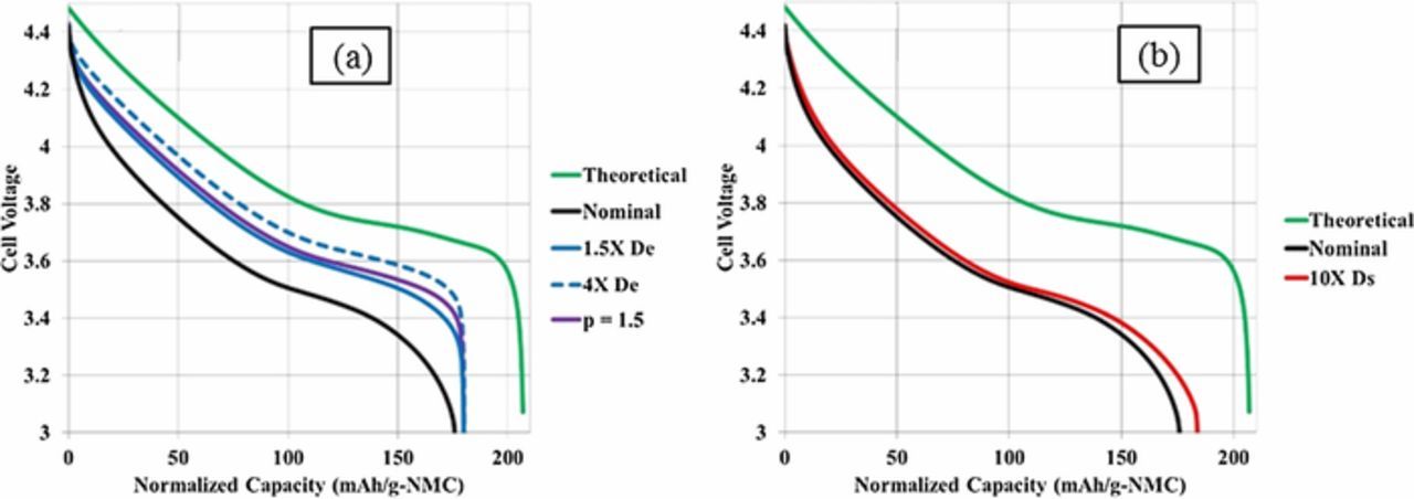
Figure 16. Macro-homogeneous model results for 1C discharge of 129-μm-thick NMC electrode 1-CAL with (a) enhanced electrolyte: (aX De) a times the nominal electrolyte diffusion coefficient and (p = 1.5) tortuosity calculated using a traditional Bruggeman exponent of 1.5 and (b) enhanced solid-state diffusion: (10X Ds) 10 times the solid-state diffusion coefficient. In both figures, the nominal (i.e., result calculated with the fitted tortuosity) and the theoretical (based on no transport losses and with a maintained open circuit voltage) curves are displayed for comparison.
Tortuosity comparison with experiment
Tortuosity factor values through the electrode thickness were determined through numerical homogenization, numerical fitting, and experimental measurements. Results are summarized in Table III and plotted in Fig. 4. The error evaluated for both methods is represented using transparent areas (cf. Fig. 4). The error determination differs fundamentally between the three methods. The homogenization error was evaluated by comparing results obtained with different numerical methods, BCs and take also into consideration the uncertainty of the CBD morphology. All these sources of error could have been determined for the 14 reconstructed volumes in an equal manner. On the contrary, the macro-homogenous model fitting approach error depends on the model sensitivity with the tortuosity parameter, which is not similar for all the samples. For instance, thin electrodes and/or those with a low tortuosity factor do not induce transport limitation except at a very high C-rate. For such materials, the macro-homogenous model is not sensitive enough to the tortuosity factor to allow an accurate determination of this parameter. Thus, the level of confidence for the fitted tortuosity factor is higher for the negative electrodes, especially the calendered ones. The experimental error does not take into consideration systematic or intrinsic errors related to the method but relies on a statistical analysis, that depends on the number of experiments, which is relatively low. It is then a difficult exercise to compare results obtained from these three approaches; hence, this caveat is kept in mind in the following section. Note that the validity of the transmission line model has been checked for microstructures made of spherical steel balls with a known tortuosity.100
Tortuosity factors for positive electrodes have been found to be fairly similar among the three methods, with the exception of one point (2-CAL) that shows a significant offset with the macro-homogenous model fitting method. Relatively poor electrochemical performance for this electrode loading, both calendered and uncalendered, was achieved compared to thicker and thinner electrode loadings. That is, the overpotential for 2-CAL and 2-UNCAL was higher than expected compared to electrodes with higher/lower loadings. The poor performance is likely due to an electrode manufacturing (cracking, insufficient mixing, etc.) or coin cell fabrication issue. Thus, this electrode likely induced an overfitting of the tortuosity factor determined by macro-homogeneous modeling.
For negative electrodes the large tortuosity induces larger observed differences between the approaches, making the error analysis even more necessary. Sample 5-CAL shows an experimental tortuosity value surprisingly lower than the one obtained for the un-calendered electrode 5-UNCAL. Macroscopic visual observation reveals the calendered sample has a large crack near the edge and a small amount of delamination of the film from the current collector. These features by themselves may not have a substantial effect on the measured tortuosity, but they could indicate or correlate with microscopic features that do have an effect. For instance, a local deficiency in the binder domain could improve ionic transport but also cause the electrode film to be more brittle and exhibit lower adhesion to the current collector. Thus, the counterintuitive trend of experimental tortuosity for the 5-CAL and 5-UNCAL samples may be influenced by undesired sample-to-sample variability.
The other seemingly anomalous electrode was 8-CAL. This relatively thin electrode showed some variability in calculated and measured tortuosities. Therefore, the polarization-interrupt method39 has been used to complement standard measurements to check the low experimental value obtained for the thin sample 8-CAL. This alternative experimental method has been repeated two times, and higher tortuosity values of τexp = 4.7 and 5.3 were obtained, more in accordance with τmicro. In general, we see good consistency between the blocking electrolyte and polarization-interrupt methods. So, the most likely cause of measurement differences is sample-to-sample variability, possibly induced by a non-uniform coating or calendering process. However, another factor that can be important is the wetting ability of the respective electrolytes used in each method. Further investigation would be required to assess why this electrode exhibits this high scattering of results.
It is remarkable that microstructure analysis and the macro-homogenous fitting method zone of confidence overlap close to the upper bound of the homogenization technique (cf. Fig. 4). Such a result suggests the morphological parameter ω of the CBD is closer to 1 than 0, as a high ω value corresponds to a higher corrective factor and thus a higher tortuosity factor (cf. Fig. 7). It indicates the CBD may be more a finger-like, nanopore network than a thin film deposited on the active material surface, as experimental observation also tends to corroborate (cf. Fig. 1a). It could also be related to insufficient electrolyte wetting for the thick electrodes. The high values obtained for both electrodes denote low Bruggeman exponent are unfit to reflect the tortuosity of the investigated mediums.
Discussion
Despite the significant differences between the three approaches used in this study, the measured values of the tortuosity factor were found to be in reasonably good agreement. Furthermore, the sources of uncertainty in each of the approaches are quite distinct from one another, but comprehensively understood for any of the methods. The main limitation to the numerical homogenization path consists in the correct determination of the CBD domain impact on the pore tortuosity. Even though a relatively narrow range is established on a corrective factor through the analysis of various geometries, future work will be needed to refine its magnitude. A direct method would consist in characterizing a volume with the CBD visible (e.g., using FIB-SEM, via backfilling to provide phase contrast). Alternatively, the morphological parameter ω could be determined experimentally, as previous modeling work has shown the cell electrochemical response depends on this parameter and could be then compared with experimental data and eventually fitted.6 The homogenization method is more reliable for low tortuosity materials as the dispersion of results, induced by the different numerical methods, almost vanishes (cf. Fig. 10). Interestingly, this low-tortuosity region corresponds to the blind spot of the numerical macro-homogenous model fitting method as the model is less sensitive to tortuosity factor for non-transport limited scenario (thin electrode and/or low tortuosity case).
On the contrary, the more sensitive the electrochemical response is to the tortuosity factor, the more accurate the error analysis performed with the macro-homogenous model (i.e., with thick and/or high tortuous materials) will be. The macroscopic model relies on assumptions to represent the particle geometries (in this case: spherical particles). While the validity of the spherical assumption can be considered reliable for the NMC electrodes, as visual inspection suggests, it is far less than adequate for the flake-like natural graphite. Therefore, the validity of the macromodel (i.e., the confidence in the results) is intrinsically different between the positive and negative electrodes, which induces a bias in the results analysis that is difficult to measure. A solution would be to work only with thick microstructures that match the morphological assumptions of the macromodel (i.e., ideally mono-size spheres packed in a regular cubic matrix, with almost no overlapping). Artificial spherical graphite could be used in this frame, at least to match the spherical assumption.
Direct experimental measurements of tortuosity likewise remain challenging as the sources of error are difficult to estimate. Even though reproducibility errors can be quantified, the intrinsic error associated with the experimental method is difficult to measure. Experiments proved to be more complicated for some un-calendered cathodes due to electronic contact issues between film and current collector (the blocking electrolyte method depends on electronic transport being much more facile than ionic transport in the sample). This suggests that the method is better-suited to calendered materials. Without an estimation of the intrinsic errors (that may differ in magnitude with different material electrode and thus being not similar among all the data points), a more reliable approach would consist in systematically using various experimental methods.67 To move forward and build confidence in the different methods, ideal electrodes for which the analytical tortuosity value is known100–102 could be manufactured (for instance using three-dimensional printing103,104) and their tortuosity evaluated. Nevertheless, the tortuosity values measured for most cathodes and anodes in this work appear to be consistent with prior measurements and trends.39
The corrective factors determined in this work are aimed amending the active material skeleton microstructure-based tortuosity factors, by taking into consideration various source of errors, mainly the absence of the CBD currently not visible with X-ray CT. They can be used to resolve the discrepancy in tortuosity factor estimation, between tortuosity factors obtained from experiments and microstructure homogenizations. Thus, it limits the need to systematically validate microstructure calculations with time-consuming experiments for similar electrode materials. For instance, Landesfeind et al.100 have measured, also with electrochemical impedance spectroscopy, tortuosity factors 1.53 to 2.01 higher than microstructure homogenization-based values, for an NMC electrode (uncertainty comes from the estimation of the segmentation error and from the repeated experiments). Authors conclude the CBD is the most likely reason for the difference but have not directly calculated the CBD impact on the tortuosity as performed in this work. Because this NMC electrode presents comparable microstructure parameter with those founded in this work (40% porosity and tortuosity from X-ray CT = 1.77 ± 0.06, similar with the sample 2-CAL, cf. Table III), the corrective factor bounds 1.42–1.81 can be used, and are in good agreement with the ratio 1.53–2.01 found by Landesfeind et al.,100 confirming the CBD is indeed the main source of error. Note the slight underestimation (1.42–1.81 vs. 1.53–2.01) may come from the higher active material weight loading used in this work (90 wt% vs 86 wt%) which reduces the impact of the CBD. The use of the corrective factors determined in the present work is relevant for other microstructures only for which both loadings and morphology are relatively similar (e.g., the corrective factor determined in this work for the graphite should not be used for spherical graphite as they have distinct microstructure).
Conclusions
Three independent tortuosity factor estimation methods (namely, microstructure homogenization enhanced with mathematically complemented CBD, macro-homogenous model fitting, and direct experimental measurements) are discussed here and have been found to be in good agreement for the investigated Li-ion graphite and NMC electrodes. This result resolves the discrepancy in tortuosity factor estimation that hindered the reliability and thus predictability of battery electrode macromodels, especially when used in transport-limited scenarios (a typical case being thick electrodes and/or fast charge, critical for automotive application).
A microstructure model has been used to calculate the tortuosity factor of calendered and uncalendered positive NMC and negative graphite electrodes based on a homogenization calculation, performed on a total of 14 microstructural three-dimensional volumes reconstructed from X-ray tomography images and enhanced with numerically generated CBD. It has been found that calendering, in addition to the expected increase in tortuosity factor due to the pore volume diminution, also provokes an increase of the anisotropy of the tortuosity factor, suggesting it may induce a particle rearrangement with the larger particle dimension getting aligned within the in-plane direction. Furthermore, the significantly high tortuosity factor anisotropy calculated for the graphite has been correlated with the graphite particle size anisotropy (related with the covariance anisotropy), indicating particle morphology anisotropy controls the anisotropy of the pore tortuosity factor. It explains, in part, the higher through-plane tortuosities calculated for the graphite compared to the NMC electrodes. The effect of the CBD on the tortuosity has been evaluated for a wide range of active material microstructures stochastically generated (considering different porosity, particle shape, orientation, and size distribution) representative of the actual negative and positive electrodes, and for a large range of CBD morphology (from a thin-film to a finger-like nanostructure). It has been found that Bruggeman's relationship cannot be extrapolated to take into consideration the effect of the CBD on the tortuosity simply by adjusting the porosity; as for the most tortuous CBD, nearly half of the tortuosity change is not predicated by the unchanged Bruggeman's law. It implies a classic Bruggeman approach is insufficient to depict the complete contribution of the CBD on the tortuosity and that Bruggeman coefficients are actually modified by the CBD. Tortuosity calculated with the CBD has been found 1.42 to 1.81 and 1.35 to 1.60 times higher than the one obtained when only the active material skeleton was considered, respectively, for the stochastically generated sphere-like positive NMC and for flake-like negative graphite electrodes with typical calendered porosities. These lower and upper bounds respectively correspond to a film-type and a finger-like CBD phase, revealing the CBD morphology and arrangement are important to accurately predict the tortuosity factor. In addition, it was found on tomography-based volumes that the tortuosity factor upper and lower bounds widen as electrode porosity decreases, suggesting CBD nanopore network geometry optimization could be valuable to improve electrolyte transport properties of high energy density (low porosity) electrodes. The bounds determined in this work could be used as a corrective factor, to multiply the tortuosity factor calculated for other battery electrode volumes obtained through X-ray CT (for which the CBD information is unknown) on the condition that their active material morphologies and volume fractions are relatively similar with the ones investigated here. Use of physics-based CBD description provides an alternative approach to account for all the relevant material phases on an X-ray CT data. Subsequent microstructural characterization allows one to consistently account for the presence of different material phases on relevant interactions such as transport in the electrolyte-filled pore network.
A CBD morphology parameter has been found to dramatically impact the CBD tortuosity factor (up to 175%). Besides, CBD reaches very high tortuosity factor and MacMullin number for the NMC cathodes, while it does not percolate for the graphite anodes. Both results could incite the battery community to revisit the implicit assumption of electronic conduction being not rate-limiting. RVE size of the CBD volume fraction and tortuosity have been found not to be related with the CBD particle size (as RVE size is commonly compared with the phase particle size), but similar to the RVE size of the macro pores, indicating the CBD nano skeleton RVE depends mainly on the heterogeneity of the spatial arrangement of the higher-scale skeleton which embeds it.
Microstructure-predicted tortuosity factors values have been validated with both macro homogenous model fitted and experimentally determined (blocking electrolyte method) tortuosity factors for the investigated volumes. The comparison was limited by the intrinsic differences between each method (as thoroughly discussed in the Results and Discussion sections), which leads to different error ranges that have to be considered to properly compare the results. In this frame, special attention has been paid to carefully evaluate the micromodel source of error (CBD unknown spatial distribution, numerical method-induced error, and porosity error). Among them, CBD has proven to be the most important, then the potential error on the segmentation, and finally the choice of the numerical method to solve the diffusion problem.
Taking advantage of the electrode capacity and cell voltage sensitivity with the tortuosity factor, the macro-homogeneous model has helped to validate the microstructure-predicted tortuosity factors, showing fitted values in good agreement. The macro-homogeneous model highlighted the need to be able to measure/predict tortuosity factors, especially when trying to maximize energy density and rate capability. Under these conditions, ion transport within the electrolyte phase becomes performance limiting, with local electrolyte depletion illustrated for a thick graphite electrode. Besides, it shows tortuosity factor impacts the capacity achievable for a given thickness and rate, which confirms the notion that accurately predicting performance requires a good estimate for tortuosity factor.
Acknowledgments
This work was authored in part by Alliance for Sustainable Energy, LLC, the manager and operator of the National Renewable Energy Laboratory for the U.S. Department of Energy (DOE) under Contract No. DE-AC36-08GO28308. Funding was provided by the U.S. DOE Office of Vehicle Technologies Energy Storage Program, program manager Brian Cunningham. A portion of the research was performed using computational resources sponsored by the Department of Energy's Office of Energy Efficiency and Renewable Energy and located at the National Renewable Energy Laboratory. The authors acknowledge Dr. Andy Jansen, Byrant Polzin, and Steven Trask of the Cell Analysis, Modeling and Prototyping (CAMP) Facility at Argonne National Laboratory for fabricating electrodes and Dr. Dennis Dees at Argonne National Laboratory for helpful discussions. The views expressed in the article do not necessarily represent the views of the DOE or the U.S. Government. The U.S. Government retains and the publisher, by accepting the article for publication, acknowledges that the U.S. Government retains a nonexclusive, paid-up, irrevocable, worldwide license to publish or reproduce the published form of this work, or allow others to do so, for U.S. Government purposes.
ORCID
Aashutosh N. Mistry 0000-0002-4359-4975
Koffi Pierre Yao Claver 0000-0003-4310-4347
Fezzeh Pouraghajan 0000-0002-9636-6714
Donal P. Finegan 0000-0003-4633-560X
Daniel Abraham 0000-0003-0402-9620
Partha P. Mukherjee 0000-0001-7900-7261
Dean Wheeler 0000-0001-5017-3194
Paul Shearing 0000-0002-1387-9531
Kandler Smith 0000-0001-7011-0377