
Abstract
The present paper seeks to extract, analyze, and interpret the electrochemical impedance spectra of a LiFePO4-Li4Ti5O12 battery to supplement state-of-charge estimation. A particular challenge in determining the state-of-charge of a LiFePO4-Li4Ti5O12 cell is that the open-circuit voltage is flat over a large range of states of charge. Because the voltage in standard batteries is typically used to inform state-of-charge estimation, a different corrective factor needs to be determined for this cell chemistry. Instead of using the battery voltage, the present study uses the battery's dynamic response to assist state of charge estimation. The present work includes at least three novel contributions: 1) the electrochemical impedance of the LiFePO4-Li4Ti5O12 cell is shown to be strongly history dependent, 2) a novel system-identification technique is implemented to extract the EIS in-situ, and 3) a signature electrochemical impedance spectra attribute is identified that is a strong function of battery state of charge.
Export citation and abstract BibTeX RIS
The primary objective of the present paper is to develop a state-of-charge (SOC) estimation technique for a lithium-iron-phosphate (LiFePO4/LFP) vs. lithium-titanate (Li4Ti5O12/LTO) battery. The LiFePO4–Li4Ti5O12 battery chemistry is of particular interest because both electrodes exhibit exceptional cyclability and safety features.1–5 However, because the half-cell open-circuit voltage (OCV) of both electrodes is flat over a large range of lithiation,3,4,6,7 the state-of-charge is difficult to determine from observable voltage. In the present study, the electrochemical impedance spectra (EIS) of a LFP-LTO cell is extracted at various states-of-charge. Subsequently, the EIS is analyzed to identify particular EIS signatures that identify state-of-charge.
This study presents at least three significant findings. First, the LFP-LTO cell EIS exhibits strong history-dependency as theorized recently by Weddle et al.8 (i.e., the EIS is not only SOC dependent, but also depends on the charge/discharge history to get to the state). Second, if the cell is charged, the EIS signatures vary with SOC at low frequencies (i.e., ω < 1 rad s− 1). However, if the cell is initially discharged, the EIS signatures vary with SOC at high frequencies (i.e., ω > 1 rad s− 1). Third, the correlation between a specific EIS feature and SOC is compared over multiple discharge cycles and multiple batteries. It is shown that if the cell is partially charged/discharged, the EIS feature can predict the state-of-charge as long as the cell state-of-charge is at a minimum relative to prior history. (That is, the cell is at the lowest state-of-charge up to that point of the cycle.)
Both LFP and LTO are typical electrodes in Li-ion batteries,4,9 albeit with LFP being much more prevalent than LTO. The lithium-iron phosphate electrode is a relatively low-voltage (nominally 3.4 V) cathode as compared to other standard cathode chemistries (e.g., LiCoO2, LiNi0.8Co0.1Al0.1O2, Li1.05(Mn1/3Co1/3Ni1/3)0.95O2), and is commonly paired with a graphite anode. LFP-graphite batteries have reduced cycle-life and safety due to the graphite's tendency to form a solid-electrolyte interface (SEI) and promote Li dendrite formation.1,10 Lithium-titanate is a relatively high-voltage anode (nominally 1.55 V) that is most commonly paired with a compensating high-voltage cathode. The high-voltage LTO anode reduces the propensity for SEI and lithium dendrite formation, but results in a lower overall battery voltage. The nominal 2 V battery is a disadvantage for the LFP-LTO cell. However, for particular applications where safety and cycle-life are paramount, the LFP-LTO pairing can be ideal.4 Additionally, both electrodes have been shown to have extremely high rate capabilities and cycle life with potential applications in ultrafast charging and high power load balancing.3,11,12
LFP-LTO state of charge estimation
State of charge (SOC) estimation is an integral component of battery management systems (BMS).13 A typical approach to SOC estimation is to monitor the current, and estimate the net charge gained or lost in coulombs by integrating the current. However, coulomb counting needs to be augmented with additional information, since 1) it only provides a relative change, so that the initial SOC must be known and 2) any bias in the current measurement will be integrated, leading to an error in the estimate SOC that increases with time. The most common supplemental information to SOC estimation is the open-circuit voltage. The open-circuit voltage is measured directly if the battery has been at rest for a sufficient amount of time. More advanced SOC estimate methods use a model based estimator that accounts for the dynamic response of the battery, and allows the updates from the voltage to occur continuously.14–16
A particular challenge in evaluating LFP–LTO battery state-of-charge is that both half-cell chemistries exhibit insignificant voltage change over large ranges of lithiation.3,6 Additionally, because both chemistries have a two-phase solid-solution insertion mechanism, both electrodes exhibit quasi-static potential hysteresis (i.e., a different voltage is measured for each electrode when the electrode is lithiated or delithiated).1,7,8,17 The two-phase solid-solution reaction also has strong memory-effect implications in LFP, which changes the observable voltage of the cathode due to partial charges/discharges, potentially leading to errors in state-of-charge estimation.18 Figure 1 illustrates the voltage profiles for a LFP-LTO cell under a C/10 demand. The figure illustrates large flat regions where the voltage is not a strong function of state-of-charge, and the hysteresis between charge and discharge demands.
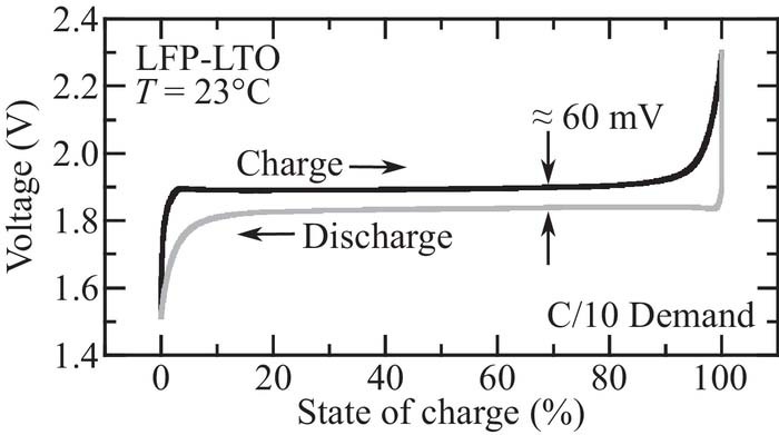
Figure 1. LFP-LTO voltage with respect to state of charge with a C/10 charge/discharge demand at T = 23°C.
State-of-charge estimation for LFP batteries with a graphite anode has been investigated previously.19–21 These papers discuss the two challenges discussed above to using the OCV as a reference for state of charge estimation: the flatness of the OCV curve, and the hysteresis that occurs between charging and discharging. In LFP-graphite batteries, the OCV decreases by about 0.1 V between 20% and 80% SOC. Since the LFP-LTO chemistry chemistry results in an OCV curve that varies less than 0.01 V between 20% and 80% SOC, the challenges are even greater.
The present paper develops an alternative to open-circuit voltage as the additional information for state-of-charge estimation in the operating region where the open-circuit voltage verses state-of-charge response is flat. The alternative presented in this study is based on observing changes in the small-signal dynamic response of the battery (i.e., the way the battery responds to a perturbation) and mapping these changes to SOC. Three well known methods to characterizing the dynamic response of batteries are the Galvanostatic Intermittent Titration Test (GITT), the Potentiostatic Intermittent Titration Test (PITT) and Electrochemical Impedance Spectroscopy.22 The PITT and GITT tests characterize the step response (with voltage or current as input, respectively), while EIS characterizes the frequency response. The variation of EIS with SOC has been noted for a variety of battery chemistries.23,24 However, these tests are usually implemented in laboratory settings.13,18 The present paper utilizes a system identification method that effectively identifies the EIS of the battery and is suitable for implementation in standard battery-management hardware (cf., In-situ EIS estimation section). Once the EIS is identified, signature features can be determined that uniquely characterize the battery state of charge.
Dependence of EIS on SOC
The present section discusses the unique EIS features of the LFP-LTO battery cell. The cell impedance is shown to not only be state-of-charge dependent, but to also have strong history-dependency (i.e., the EIS at a particular state-of-charge depends on the previous charge/discharge history). All experimental results are obtained using 26650 format LFP-LTO batteries manufactured by K2 Energy (Henderson, NV) with nominal capacity of 2100 mAhra. The present section presents results generated from a Gamry Interface 1010E potentiostat/galvanostatb with voltage-perturbation amplitudes of 5 mV. The impedance is extracted after a two-hour rest between the charge/discharge demand, which is a similar rest time to foregoing experimental studies.19
Figure 2 illustrates EIS measurements at various states of charge. In the experiment, the cell is monotonically charged/discharged by 10% SOC increments and rested for 2 hours followed by the EIS measurement. Figures 2a, 2c, and 2e illustrate the extracted EIS for the monotonically charged cell and Figs. 2b, 2d, and 2f illustrate the EIS for the monotonically discharged cell. The cell EIS is taken at 0°C (Figs. 2a–2b), 23°C (Figs. 2c–2d), and 46°C (Figs. 2e–2f). The Nyquist plots illustrate frequencies from 10 kHz to 10 mHz.
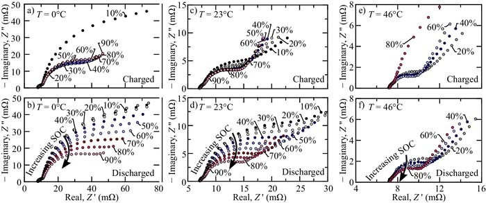
Figure 2. Electrochemical impedance spectra of an LFP-LTO cell at multiple states of charge and temperatures. The bottom figures (i.e., (b), (d), and (f)) illlustrate the EIS of a discharged cell, while the top figures (i.e., (a), (c), and (e)) illustrate the EIS of a charged cell. The EIS is identified at three operating temperatures: T = 0°C (a-b), T = 23°C (c-d) and T = 46°C (e-f).
There are at least three significant EIS attributes that can be interpreted from Fig. 2. The first is that the cell EIS is temperature dependent. For example, Fig. 2a is significantly different from Fig. 2c or Fig. 2d. It should be noted that temperature dependence is expected in the EIS curves. Generally, the internal resistance of the cell (due to both transport and kinetics) decreases with increased temperature and visa versa. The second significant attribute is the cell impedance is different if the cell is discharged or charged to a particular state of charge. For example, the impedance of Fig. 2a is significantly different than Fig. 2b. History-dependent state of charge has been theorized previously for cells with phase-transformation electrodes.8 The history-dependency EIS is most evident at low temperatures (cf., Figs. 2a–2b) and is much less evident at higher temperatures (cf., Figs. 2e–2f). Finally, at nominal or cool temperatures, the discharged cell EIS is strongly correlated to the state of charge. For example, Fig. 2d illustrates the EIS of a discharged cell at nominally room temperature. As the battery state-of-charge increases, the first prominent characteristic semi-circle arc decreases (i.e., the semicircle with frequencies just above ω > 1 rad s− 1). The strong EIS-SOC depedency is further indicated by a black arrow denoted "Increasing SOC" in Figs. 2b–2d, and 2f.
An important objective of the present paper is to identify a EIS-SOC relationship that can supplement in-situ state-of-charge estimation via coulomb counting. For these purposes, a monotonically charged cell (Figs. 2a, 2c, and 2e) exhibits weak EIS-SOC dependence. In fact, the different state-of-charge impedances are difficult to label because the EIS are so close. Although there doesn't seem to be a significant trend correlating SOC to the measured EIS for a charged cell, it may be the case that low frequency behavior (i.e., ω < 1 rad s− 1) contains a unique EIS-SOC relationship. However, such low frequency identification is impractical for real-time state-of-charge estimation. Conversely, continuously discharged cells show strong EIS-SOC relationships. Specifically, the contact resistance is independent of SOC, and the first semicircle arc radius decreases with increasing state-of-charge.
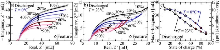
In the present study, a single EIS feature is chosen to uniquely identify the state of charge. It should be noted that the singular feature chosen in this study may not be the most representative and that further study is required to accurately represent a unique EIS-SOC relationship. Nevertheless, the unique EIS chosen to supplement SOC estimation is the maximum (negative) impedance above 1 rad s− 1. The maximum (negative) impedance is chosen here because it has important implications in standard equivalent circuit analysis. The maximum (negative) impedance of the first semicircle is related, in equivalent circuit analysis, to the charge-transfer resistance of an electrode. The maximum (negative) impedance has the added benefit of being independent of the contact resistance, which can change with measurement equipment.
Figure 3 illustrates the maximum (negative) impedance above 1 rad s− 1 for the discharged LFP-LTO cell at 0°C (cf. Fig. 3a) and 23°C (cf. Fig. 3b) with respect to state of charge. Note that in some cases, the first semicircle is not well defined, so the the maximum is taken at 1 rad s− 1. As illustrated, and discussed previously, the maximum negative impedance decreases with increasing state of charge (cf. Fig. 3c). This "mapping" between the EIS and SOC is used in the following sections. However, instead of relying on standard sinusoid perturbations to extract the EIS, a procedure is developed to identify the state of charge in-situ. The following section develops a method for in-situ EIS estimation, which in-turn provides a means to estimate the state of charge.
In-Situ EIS Estimation
System identification is the extraction of a dynamic model using data. System identification has been applied in battery systems, although typically the resulting model is used to predict the current/voltage time response.25–30 The frequency response of the identified model provides an estimate of the impedance spectrum, and thus system identification is also a useful method for implementing an EIS measurement in the field.8,31–33 The specific system identification method used here is a maximum-likelihood method, and is similar to prior work.31–33 However, the present work includes at least two novel sytem-identification elements. The novel elements added for accurate system identification (and thus EIS estimation) include 1) using a Kalman Filter to calculate the likelihood while accounting for noise in both the voltage and current measurements, and 2) using a parameterized continuous-time model so that multiple experiments with different sample rates can be used simultaneously.
To identify EIS signature features for SOC estimation for practical applications, the EIS must be determined using standard battery management system (BSM) equipment. In the present study, EIS identification of a cell using standard BMS equipment is referred to as in-situ identification. In-situ identification is characterized by measuring the voltage trajectory of the battery in response to an on/off transient load. One way a small transient load can be easily applied is via a passive balancing resistor, which is standard in BMS. In the present study, a National Instruments USB-6211 16 bit DAQ is used to measure battery voltage and control the applied current via operational amplifiers controlled transistor pairs (cf., Fig. 4). While the equipment used in the present study can apply to any current perturbation, a binary current perturbation is used for identification to mimic the effect of turning on and off a balancing resistor. All in-situ EIS estimation experiments are tested at T = 23°C.
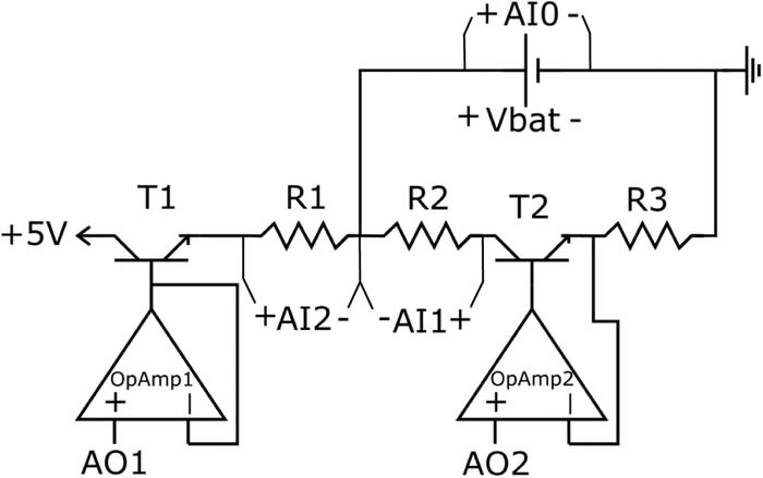
Figure 4. Test circuit diagram. "AO#" indicates a voltage output of the DAQ and "AI#" indicates a voltage input to the DAQ.
Figure 5 illustrates an example current and voltage sequence used in the present study. The voltage response is normalized to zero mean. Note that if a balancing resistor is utilized, the current does not need to be measured, as its value can be calculated from the voltage and resistor size. Figure 5 illustrates the time response of a discharged LFP-LTO battery at three different SOC. Although there are some differences in the observed voltage perturbations for the three states of charge, the differences are slight. Additionally, the small-amplitude current perturbation results in an observed voltage with a low signal-to-noise ratio. To accurately identify the battery input-output (i.e., current-voltage) response, the data needs to be processed before extracting the EIS.
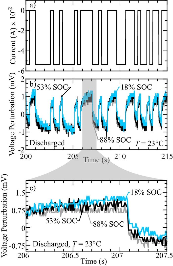
Figure 5. Pseudo-random binary sequence current perturbation and voltage response of an LFP-LTO battery at T = 23°C. The voltage response for three different states of charged are superimposed on the lower subplots.
The data processing method presented here is based on system identification, which finds the dynamic system which best explains the measured data, with "best" determined under a criterion explained below. To ensure the identified model accurately represents the battery's wide-bandwidth frequency response,8 multiple current perturbation sequences, with different switching times, are utilized. In other words, at a particular state-of-charge, several small-signal current perturbation tests are imposed, each with a different on/off switching time. At the "switching time" the current can change from on to off (or vice versa). Whether or not the switch occurs is decided by a pseudo-random binary sequence.34 The current-voltage response identified at the on/off switching time accurately describes a portion of the battery frequency response near the switching frequency. In the present study, switching times of 32, 320, and 1000 ms are chosen. For each test, 25 samples are taken for each potential on/off switch at the slower switch times (i.e., sampling at =320/25 and =1000/25 ms, respectively) and 4 samples per on/off switch at the fastest switch time. The relatively high sampling rate at the slower switching times increases the signal-to-noise ratio.
System identification is implemented using a maximum-likelihood approach with a parametric continuous-time model. The continuous-time model in transfer function form may be expressed as
![Equation ([1])](https://content.cld.iop.org/journals/1945-7111/166/16/A4041/revision1/d0001.gif)
with parameters
![Equation ([2])](https://content.cld.iop.org/journals/1945-7111/166/16/A4041/revision1/d0002.gif)
where s = jω,  , ω is frequency, and pn and zn are poles and zeros of the transfer function G. For fixed θ, given a (current) input sequence
  applied at sampling time Ts, the model can predict the output (voltage) sequence
  . Suppose there are N experiments, each with a different sampling rate, with the experiment number indexed by ℓ, and the experimental current and voltage sequences is denoted as uℓk and yℓk, respectively (in the present study N = 3). The parameters θ are estimated using the optimization problem
![Equation ([3])](https://content.cld.iop.org/journals/1945-7111/166/16/A4041/revision1/d0003.gif)
where for vector x,  is the weighted Euclidian norm. Equation 3 is a maximum-likelihood estimate of θ when the current and voltage measurements are perturbed by zero mean white Gaussian noise with covariances Q and R, respectively.35 The inner minimization is solved using a Kalman filter,36 while the outer minimization is solved using gradient descent. The inner minimization can be thought of as ensuring that the current-voltage dynamics match the dynamics of G(s, θ) for a particular test ℓ. The outer minimization can be thought of as ensuring that the parameters θ chosen for all tests ℓ are self-consistent. Once the parameters θ are identified, the EIS estimate at frequency ω is
![Equation ([4])](https://content.cld.iop.org/journals/1945-7111/166/16/A4041/revision1/d0004.gif)
Since gradient descent is used and the optimization problem is non-convex a good initial estimate of θ is required. A "good" initial estimate of θ is provided to the solver by first fitting discrete time output error (OE) models35 to the fastest and slowest switching time data sets. The OE model is then converted to continuous time. The real pole-zero pairs are extracted from the continuous-time model that have a magnitude greater than 1/(1000Ts) and have a ratio of Z''/Z' (i.e., Im/Re) less than 0.2. The number of these pairs determines n, and their value is used to initialize the gradient descent algorithm (cf., Eq. 2).
To illustrate typical performance, Figure 6 shows the LFP-LTO battery EIS extracted using sinusoids and the in-situ identification method at three different states of charge. After an identification experiment, sinusoidal current perturbations are applied at 10 frequencies between 0.6 and 150 rad s− 1, with the amplitude and phase shift determined using a correlation analysis. The EIS obtained via system identification and via sinusoidal analysis shows excellent agreement (cf., Fig. 6). It should be noted that although the EIS identified using the system identification method is plotted using dots, the method actually provides an estimate at any frequency, and thus is more appropriate for determining a signature EIS feature to determine SOC (e.g., maximum imaginary part).
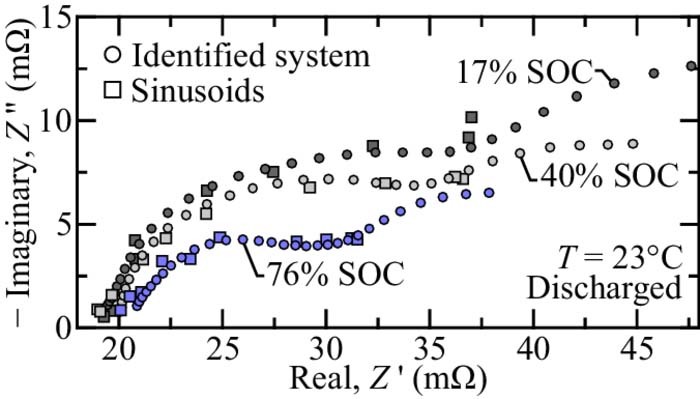
Figure 6. Electrochemical impedance spectra of a discharged LFP-LTO cell at three different states of charge at T = 23°C. Circles indicate impedance predicted by the identified system. Squares indicate impedance extracted using sinusoid perturbations.
Monotonic Discharge Demands
In-situ identification experiments are imposed on two different LFP-LTO cells. In these experiments, the battery is discharged to the desired state of charge using a 1 C current, followed by a rest period of 60 min. It should be noted that the cell may not be fully relaxed after an hour, but that further relaxation will not dramatically change the observed EIS.37 This is also verified experimentally in EIS evolution with relaxation time section. Perturbation experiments are then imposed and the current and voltage are recorded. A system G(s, θ) is then determined that accurately represents the current-voltage dynamics (Eqs. 1–3). Once a system is determined, the electrochemical impedance is identified and the maximum (negative) imaginary impedance is extracted.
For each (discharged) EIS estimate, the magnitude of the maximum negative imaginary part of the impedance for frequencies greater than 1 rad s− 1 are determined. Figure 7 illustrates cell state of charge with respect to the signature EIS feature. Three cell responses are plotted. The circles and triangles (denoted "Cell 1" and "Cell 2", respectively) are cell responses identified using the in-situ method described in In-situ EIS estimation section. The cell response denoted "Gamry identified cell" are extracted using the sinusoid responses illustrated in Fig. 2b and Fig. 3. Figure 7 shows an excellent correlation between SOC and the impedance feature, especially at higher states of charge. It should be noted that each cell in Fig. 7 has a slightly different slope. The slightly different slopes of the state of charge with respect to the signature EIS feature indicates that greater accuracy can be achieved by calibrating the relationship to a particular cell. Such individual cell calibration is similar to what is done for SOC estimation using open circuit voltage.
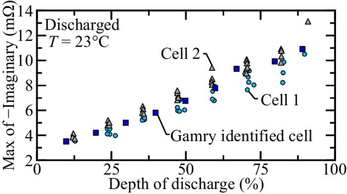
Figure 7. Comparison of max negative impedance feature and depth of discharge for three different LPF-LTO cells.
Nonmonotonic Charge Demands
The foregoing sections determine an EIS signature that uniquely identifies a monotonically discharged cell state-of-charge. However, because the cell EIS has such strong history dependency (cf., Fig. 2), there is value in quantifing the EIS response of cell that has a nonmonotonic current demand history. Of course, there are numerous potential nonmonotonic current demands to evaluate. The present study focuses on the EIS response of a cell that undergoes a predominately discharge demand with intermittent charging demands.
Figure 8a illuastrates the nonmonotonic demand chosen for the present study. Illustrated is the cell state-of-charge set-point with respect to test number. The systematic charge/discharge demand between tests is as follows
- (1)Discharge the cell by ∼ 12% SOC (cf., ○ in Fig. 8a)
- (2)Charge the cell by ∼ 12% SOC (cf., △ in Fig. 8a)
- (3)Discharge the cell by ∼ 3% SOC (cf., ◊ in Fig. 8a)
- (4)Repeat (3) five more times (cf.,
 , ⬠, etc., in Fig. 8a)
 - (5)Restart the procedure.

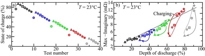
Figure 8. Figure (a) illustrates the state-of-charge with respect to test number. Figure (b) illustrates the maximum (negative) impedance above 1 rad s− 1 for each of the tests with respect to state of charge.
For each test, the cell is charged/discharged to the state of charge indicated on the graph at a 1/10 C rate and allowed to rest for 1 hr. After the cell has relaxed, the EIS is extracted using the in-situ method (cf., For each test, the cell is cha section). The cell is then charged/discharged to the proceeding state of charge for the next test. For easy visualization, the symbols in Fig. 8 change color each time the test procedure is repeated.
Figure 8b illustrates the maximum (negative) imaginary impedance above 1 rad s− 1 of the in-situ EIS identified for each test. The black dotted line overlaid on the figure is the linear EIS-SOC response of a monotonically discharged cell (cf., Fig. 3). Focusing on the red tests, the first (discharged) test (illustrated as a red circle) has a very similar EIS-SOC feature as compared that of the monotonically discharged cell. Once the cell is partially charged (illustrated as a red triangle) the EIS-SOC feature decreases magnitude dramatically and deviates far from the monotonic response. As the cell is slowly discharged in the following tests, the EIS-SOC feature approaches the monotonic discharge curve. When the cell is returned to the same state of charge as before the charging test (illustrated as a four-point star), the EIS-SOC feature is the same as that of the monotonic discharge demand. The last two tests in the sequence (illustrated as a five-point and six-point star, respectively) remain close to the EIS response of the monotonically discharged demand. A significant observation is that if the cell is at its most discharged state during the nonmonotonic cycle, the EIS-SOC feature is independent of previous charge/discharge history. In other words, the cell EIS-SOC feature tends to "forget" intermittent charge once the charged capacity is discharged. The gray, green, and blue sequences have the same trends as the red sequence. At high states of charge (black sequence), the EIS-SOC response is relatively indifferent to the charge history demand.
A reason why the EIS-SOC feature "forgets" intermittent charging demands after the charged capacity is discharged can be explained through the lens of a mesoscopic model.8,38,39 The mescopic model represents an electrode as an ensemble of particles that vary with size and charge-transfer resistance. In the mesoscopic model, smaller particles that have less charge-transfer resistance are the first to receive/donate lithium from/to the surrounding electrolyte during charge/discharge demands. When continuously discharging, small particles are the first to lithiate(cathode)/delithiate(anode). After the small particles lithiate/delithiate, the large, highly charge-transfer resistive particles will being to lithiate/delithiate.8 When the cell is intermittently charged, the small particles are the first to delithate(cathode)/lithiate(anode). Because the small particles are most active during the system identification perturbations,8 the EIS of the intermittently charged cell is dominated by the response of these smaller particles, and the overall EIS appears similar to the response of a cell that has been monotonically charged by an equivalent amount (cf., Fig. 2c). When the cell is slowly discharged after the intermittant charge, the small particles are again the most active and lithiate(cathode)/delithiate(anode) reducing their effect on the EIS. Finally, once the capacity gained from the intermittent charge is discharged, the lithium distribution within the electrode ensembles appears as if the cell were monotonically discharged.
EIS Evolution with Relaxation Time
A potential critique of the SOC estimation presented in the present study is that the EIS may change with relaxation time. In other words, it may be the case that the EIS changes after the cell has rested with no current demand. In the present study, the EIS is extracted after 2 hr relaxation in the Gamry Interface 1010E Potentiostat experiments (cf. Figs. 2, 3, and 7). However, the in-situ identification (cf., In-situ EIS estimation, Monotonic discharge demands, and Nonmonotonic charge demands sections) are taken after 1 hr relaxation. To ensure the cell is fully "relaxed" after 1 hr, the cell impedance is extracted at various relaxation times. Figure 9 illustrates the EIS for a representative relaxation experiment. The figure illustrates the extracted EIS from a discharged cell at 50% SOC at room temperature using the in-situ identification method presented in In-situ EIS estimation section. The EIS is extracted immediately after a 1 C discharge (labeled 0 hr), and after 1 hr, 2 hr, 3 hr, 5 hr, and 11 hr of relaxation. Aside from the 0 hr case, which has a significantly different EIS, all other extracted EIS are generally the same. There are some slight differences in the low frequency behavior (i.e., ω ⩽ 1 rad s− 1) with increased relaxation times, but the slight changes do not significantly influence the relatively "high-frequency" semicircle arc radius. Because the high-frequency dynamics do not change after 1 hr relaxation, the EIS-SOC feature can be used to accurately predict SOC with relatively short (i.e., 1 hr) relaxation times.
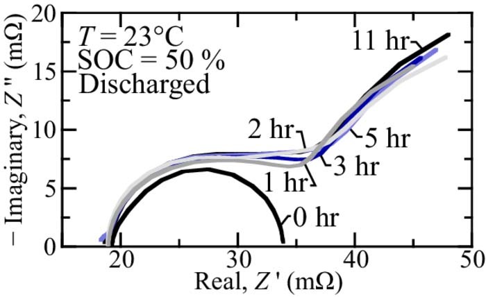
Figure 9. In-situ EIS extracted at 50% SOC and T = 23°C at various relaxation times over 0.1 rad s− 1 ⩽ ω ⩽ 400 rad s− 1.
Conclusions
Over a large portion of their operating range, LPF-LTO batteries have a open circuit voltage that is nearly flat, limiting the usefulness of cell OCV for SOC estimation. Fortunately, the dynamic response of the battery, as characterized by the EIS, does vary with operating point, and provides an alternate signpost for SOC estimation. A complicating factor is the LFP-LTO cell exhibits strong history-dependency (i.e., the EIS changes if the cell has been discharged or charged). The current study found that the EIS of a discharged cell has strong SOC dependence at reasonably fast frequencies (i.e., ω > 1 rad s− 1). Because of this strong EIS-SOC dependence, the current study focuses on estimating the SOC of a discharged cell, or at points of discharge where the SOC is at a low-point relative to the past cycle history. A signature feature of the EIS curve (the maximum (negative) impedance of the first semicircle) is identified as a feature in the EIS response that uniquely defines the battery state of charge. Additionally, a novel system-identification method is devised that accurately identifies a batteries current-voltage (i.e., EIS) response using simple on/off current switching. The system-identification provides a method to efficiently extract a battery's EIS (and thus correlating SOC) in-situ. Future work will consider state-of-charge estimation for charged LFP-LTO cells. Such estimation techniques will require estimating the EIS accurately at frequencies lower than 1 rad s− 1, as well as SOC estimation at other points along partial charge/discharge trajectories.
Acknowledgments
The present work is supported by the Office of Naval Research via grants N00014-16-1-2780 and N00014-17-1-2697. EIS measurements were conducted at Naval Surface Warfare Center Carderock Division with support from the Office of Naval Research via grants N0001418WX01538 and N0001419WX01258. The authors thank Dr. James Hodge and K2 Energy for assistance in the development of this paper.
ORCID
Peter Weddle 0000-0002-1600-0756
Miaomiao Ma 0000-0001-5719-6102
Christopher Hendricks 0000-0002-7358-1948
Robert Kee 0000-0003-3930-4784
Tyrone Vincent 0000-0002-6921-8521
Footnotes
- a
Part number: 18x0601.
- b
Gamry Instruments Inc., Warminster, PA.